Double coverage and demand for health care:
Evidence from quantile regression
Sara Moreira
Banco de Portugal, ISEG-TULisbon
Pedro Pita Barros
Universidade Nova de Lisboa
May 1, 2009
Abstract
An individual experiences double coverage when he bene…ts from more than one health
insurance plan at the same time. This paper examines the impact of such supplementary
insurance on the demand for health care services. Its novelty is that within the context of
count data modelling and without imposing restrictive parametric assumptions, the analysis
is carried out for di¤erent points of the conditional distribution, not only for its mean location.
Results indicate that moral hazard is present across the whole outcome distribution for
both public and private second layers of health insurance coverage but with greater magnitude
in the latter group. By looking at di¤erent points we unveil that stronger double coverage
e¤ects are smaller for high levels of usage.
We use data for Portugal, taking advantage of particular features of the public and private
protection schemes on top of the statutory National Health Service. By exploring the last
Portuguese Health Survey, we were able to evaluate their impacts on the consumption of
doctor visits.
Keywords: Demand for health services, Moral hazard, Count data, Quantile regression.
JEL codes: I11, I18, C21, C25
1
Introduction
The aim of this paper is to analyse the impact of health insurance double coverage (i.e. a situation
in which an individual is covered by more than one health insurance plan)1 on the consumption
of health care. It is well known that if the demand for health care reacts to budget constraints
and preferences changes then, double coverage should also have important e¤ects because it
modi…es the actual price of services, the income of the insured, and the opportunity cost of time
in the case of illnesses. The e¤ect of supplementary health insurance is often associated to an
aggravation of moral hazard that creates incentives for people to go to the doctor more frequently
and eventually because of less severe illness.2
Organizational designs of health systems may generate layers of coverage. The most common
situation regards the case where an individual bene…t from a compulsory public insurance, and
in addition he has purchased a private one. Such supplementary private health insurance usually
overlaps the range of health care services provided by the statutory health system. The main
purpose of second (and higher) layer of coverage is usually to increase the set of choices about
the health care provider (for example, private providers or private facilities in public institutions)
as well as to decrease the level of co-payments done by the individual. By increasing the choices
of provider, patients may also obtain a faster access to health care. Quantitatively, double
coverage is not a negligible phenomenon. It can be found in all European countries, being
common in Finland, Greece, Portugal, Spain, Sweden and in the United Kingdom. Furthermore,
in the United States, the Obama plan is expected to increase health coverage, inclusively by
allowing Americans to maintain their current insurance scheme while accessing new options.
In such scenario, double coverage situations are expected to augment signi…cantly in coming
years. Research on this phenomenon can help to detect whether possible ine¢ciencies, causing
unnecessary and costly utilization due to moral hazard, should be a concern.
Existing works addressing health insurance double coverage focus on mean e¤ects. In
con-trast, by looking at other points of the conditional distribution we unveil that stronger e¤ects
1The terms "duplicate coverage", "supplementary health insurance" or "additional health insurance" are used
alternatively in the literature.
2Moral hazard in this context is de…ned as the "change in health behaviour and health care consumption caused
by insurance" (Zweifel and Manning 2000). Some authors criticize the direct association of double coverage with moral hazard, arguing on the existence of other important e¤ects. For instance, Vera-Hernández (1999) refers the impact of the insurance on the health status of the individual, which will decrease the future consumption of health care. Also Coulson et al. (1995) points to existence of supply-inducement by providers.
are found for less frequent users. Our …ndings are the result of the application of an innovative
technique for estimating the quantile regression for counts. The estimates were computed with
Portuguese data3, using as source of double coverage the existing health insurance schemes
be-yond the National Health Service (NHS). Approximately a quarter of the Portuguese population
has access to a second (or more) layer of health insurance coverage on top of the NHS, through
mandatory (occupation-based) health subsystems for workers of some large companies and public
employees and voluntary health schemes. We focus our attention on the double coverage resulting
from the former type, regarding both health insurance plans provided to public employees and
insurance plans of private companies. Results indicate that double coverage is especially high
in the private subsystems (2.6 to 2.9 times higher than the one presented by public employees).
An interesting …nding, which could only be observed through the use of quantile analysis, is that
these e¤ects are lower in the upper tail of the outcome distribution. This shows that health
insurance double coverage is relatively more relevant for the …rst levels of usage since for more
frequent users the consumption behaviour depends less on the health insurance plan.
We measure health care demand through the number of doctor visits during three months.
As in most of the research on health care, the dependent variable is a non-negative integer count
characterized by a large proportion of zeros, a positive skewness and, as a consequence, a long
right hand tail. In what concerns to the econometric tools, until recently, the one-part, Hurdle
and …nite mixture models have dominated the empirical literature (Deb and Trivedi 2002).
Estimators resulting from these frameworks rely on assumptions about the functional form of
the regression equation and the distribution of the error term. As a result, standard models
determine entirely the distributional behaviour by the functional form once the conditional mean
response is known. An attractive alternative is the usage of nonparametric and semiparametric
estimators. Introduced for continuous data in Koenker and Bassett (1978), Quantile Regression
o¤ers a complete picture of the e¤ect of the covariates on the location, scale and shape of the
distribution of the dependent variable. As a semiparametric method it assumes a parametric
speci…cation for the quantile of the conditional distribution but leaves the error term unspeci…ed.
It was …rst applied to continuous health data in Manning et al. (1995). As in Winkelmann
(2006) and Liu (2007), we apply an approach suggested by Machado and Santos-Silva (2005) in
3In particular, the Portuguese Health Survey of 2005/2006, a cross sectional health dataset that provides a
which quantile regression is extended to count data through a "jittering" process that arti…cially
imposes some degree of smoothness. This technique allows an analysis of the e¤ect on the whole
consumption distribution, which is an important step forward in the analysis of reforms and
is very useful for policy making. In particular, it may help the policy maker to understand
why people with similar health conditions di¤er in their use of medical care, since it enables to
determine whether the policy e¤ect is larger among low users or among high users, or may even
signal the need for adjustments on the characteristics of the contracts provided by the insurances
companies. This kind of information is important to control the expenditures in health care as
well as to assess the equity of the system.
Many authors have been investigating the impact of additional health coverage in order to
estimate the moral hazard derived from di¤erent health insurance plans characterized by di¤erent
levels of coverage (for example Cameron et al. 1988, Coulson et al. 1995, Vera-Hernández 1999,
Lourenço 2007 and Barros et al. 2008). The usage of non-experimental data generally creates an
endogeneity problem related to adverse selection since most of the times the decision to buy extra
health insurance depends on individual characteristics. In such cases, the insurance parameter
does not disentangle moral hazard and adverse selection e¤ects. The solution relies most of the
times on …nding reasonable instrumental variables. Our empirical application does not have this
problem because the membership on public and private health subsystems was mandatory and
based on professional category, meaning that they were unrelated to the expected value of future
health care consumption. Note that we are excluding from the analysis the voluntary health
insurance plans.
The paper is structured as follows. Section 2 describes the Portuguese health care system
from a provision perspective. Section 3 describes the dataset and the relevant variables, and
presents an exploratory analysis of the data. In Section 4 we present the quantile regression for
counts and discuss the treatment e¤ect speci…cation. In Section 5 we analyse the results and
2
Portuguese health care system: an overview from the
provi-sion perspective
The Portuguese health system is a network of public and private health care providers and
di¤erent funding schemes.4 It is possible to identify three overlapping layers: the National
Health Service (NHS)5, mandatory public and private subsystems and private voluntary health
insurance. While the NHS is mainly …nanced by general taxation, subsystems resources come
from employees and employers compulsory contributions (including, in the public schemes, State
funds to ensure their balance). According to Barros and Simões (2007), in 2004 public funding
represented 71.2 per cent of total health expenditure (of which 57.6 per cent is related with
the NHS and 7.0 percent cent with subsidies to public subsystems). Private expenditure is
composed by co-payments and direct payments made by patients and, to a lesser extent, by
private insurance premiums.
Since 1979, with the creation of the NHS, legislation established that all residents have the
right to health protection regardless of economic or social status. Until then, the State had full
responsibility only for the health care of public employees and some speci…c types of services,
as maternity, child and mental care and the control of infectious diseases. One of the features
of the period preceding the outset of the NHS that persisted was the existence of public health
subsystems, partially because trade unions, which managed some of those subsystems, were not
willing to give up their privileges and forcefully defended their maintenance on behalf of their
members (Barros and Simões 2007).
The individuals covered solely by the NHS (the majority of the population) face some
con-straints in the access to public providers, in particular because of services excluded from the
public network and di¢culties of access due to time costs (long waiting lists and queuing) or
geographical barriers. Lourenço (2007) among others, argues that the NHS coverage restrictions
convert its normative completeness into an incomplete health insurance contract. The NHS is
conceived in a way that bene…ciaries should …rst seek health care through their general
prac-4This section is mostly based on Barros and Simões (2007) and Lourenço (2007). An interesting comparison
between the Portuguese health system and other European systems is available in Bago-d’Uva and Jones (2008).
5In the autonomous regions, the public health is ensured by regional health services (RHS of Azores and
titioner (family doctor) in health care centers and then, if necessary, get appropriate referrals
to a public specialist consultation (generally as out-patient consultations in public hospitals).
This gatekeeper procedure is not strictly followed since there are households who do not have
access to a family doctor and, when they have, the time lag between the …rst step to obtain
health care and its e¤ective provision is frequently too long. Additionally, the requirements to
obtain referrals are generally very demanding. For these reasons, some individuals have their
…rst contact with health care in hospitals’ emergency rooms even if their condition would not
require it. Given this constraints, the consumption of private services by NHS bene…ciaries6 is
very common. The NHS design contemplates a cost-share mechanism that in practice makes
the patients pay a mandatory small co-payment to the public provider (variable with the type
of service), usually on a fee-for-service basis. There are, however, exemptions for a large share
of the population de…ned on the basis if the age and income distribution. When using health
services provided by the private sector, NHS bene…ciaries, in the absence of private voluntary
insurance schemes, support their full cost, having no reimbursement for it.7 People who bene…ts
from additional health care schemes, either mandatory or voluntary, do not see their taxation
a¤ected, and as a consequence they are still eligible to receive health care from the NHS.
Nowadays, a considerable share of the population (between 20-25 per cent of overall
popu-lation) still bene…ts from occupation-based health insurance through several subsystems, either
private or public. Among the double coverage’ schemes, the largest public subsystem is ADSE
(Direcção-Geral de Protecção Social aos Funcionários e Agentes da Administração Pública), a
Government department acting as a health insurance provider, covering public employees (about
15 per cent of the population). Exceptions enjoying speci…c schemes also exist, like the
mil-itary personnel. Private subsystems were created to workers and pensioners (and respective
households) of private companies that have their own insurance schemes, like SAMS (Serviços
de Assistência Médico-Social) for banking employees. Each subsystem has a distinct array of
medical care insurance arrangements to …nance and provide health care. As a whole, we can say
that they are organized di¤erently from the NHS, in particular because of the lower proportion
of services directly provided. They basically provide health care through contracts with
pub-6In the course of the paper, when it says "NHS bene…ciaries", we consider individuals covered solely by NHS.
Therefore, this de…nition excludes the population with double coverage.
7The system allows, however, the recovery of some out-of-pocket outlays because both patient co-payments and
lic/NHS and private institutions and reimburse patients costs for services supplied by private
entities without contract. These features make these schemes more comprehensive health
protec-tion plans than NHS, representing both complementary and supplementary types of insurance
(Lourenço 2007). The supplementary protection results from the provision/…nancing of services
that are also available in the context of the NHS. This particular feature creates the double
cov-erage problem. The complementarity characteristic is relevant due to the fact that subsystems
cover services almost not provided by the general system, in particular, by reimbursing part of
patients costs in private providers (even the ones without contracts).
3
Data
3.1 Dataset
Data was taken from the fourth Portuguese Health Survey (PHS), a cross sectional health dataset
designed to be representative of the Portuguese population that lives in households.8 It provides
a wide range of information at an individual level, namely demographic and socioeconomic
conditions, type of health insurance, health-care utilization, health status indicators (like chronic
diseases and long run and short run disability), lifestyles (like alimentation habits and sports
activity) and costs with health services. However, some of the questions were only answered by
part of the sample. The survey was collected by interviews carried out between February 2005 and
January 2006. The PHS sample re‡ects the geographical structure of the population according
to the 2001 census, resulting from a two-stage cluster sampling that followed a complex design
involving both strati…cation and systematic selection of clusters.9 A total of 19,950 households
units were selected for the survey. In each household all individuals were face-to-face interviewed.
The sample used in this paper comprises 35,308 observations and was obtained after treating
the data and imposing some constraints. Firstly, we excluded 158 observations of individuals
that did not report the number of visits to a doctor, 10 observations without answer regarding
the subsystem they belong to and 3,114 observations of persons with voluntary private health
8The PHS are carried out by the Portuguese Ministry of Health in collaboration with National Health Institute
Ricardo Jorge and National Statistics Institute. Until now, four questionnaires have been made (1987, 1995/1996, 1998/1999 and 2005/2006) using probabilistic samples of the continental population (1st. 2nd and 3th PHS) and of both continental and autonomous regions of Azores and Madeira population (4th PHS). Here we made use of the last available questionnaire. Note that it is not a panel survey since the sample changes between surveys.
insurance. Secondly, we dropped 145 observations of pregnant women whose visits to the doctor
were related to their condition. Finally, we deleted 1,047 observations with missing values for
any other relevant variables (according to the set of regressors chosen).
Three points should be made to the latter choices. Firstly, the simplest way of handling
missing data is to delete them and analyze only the sample of "complete observations" (although
deleting observations reduces the e¢ciency of the estimation). This procedure is named aslistwise
deletion. Its usage is statistically appropriate only if the missing values are missing completely
at random (Cameron and Trivedi 2005), which means that the probability of missing does not
depend of its own value nor on the values of other variables in the data set (the observed sample
is a random subsample of the potential full sample). Among the relevant questions of our dataset
that can create a sample selection problem, the one that generated more missing observations
concerns the income level. However, most of the missing (around seventy per cent) does not
result from a non answer but from individuals that declare not knowing the household income,
which if not deliberately makes unlikely that unobserved factors in‡uenced both the decision to
respond and the value of the dependent variable.
Secondly, the exclusion of voluntary health insurance individuals can be pointed as a
short-coming. The problem is that including such variable may introduce endogeneity problems,
dif-…cult to eliminate since there are no suitable instrumental variables (Barros et al. 2008). In
this context and given the relatively small number of insured individuals (7.6 per cent) it seems
better to exclude such observations and restrict the analysis to the population exclusively insured
through mandatory schemes.
Finally, another important feature that is worth noting is that the database has weight
variables (natural in a sample created to be representative of the population). It is possible to
ignore them without a¤ecting the parameter estimates (Wooldridge 2002, Cameron and Trivedi
2005). This is more likely, when sampling weights are solely a function of independent variables,
or when the model can be respeci…ed (including new variables or interactions). Otherwise,
parameters estimated would be biased. The problem with the use of a weighted dataset is that
it leads to arti…cially small standard errors for regression coe¢cients and therefore incorrect
inferences on the signi…cance of the di¤erent e¤ects. We chose to exclude the weights from the
3.2 The variables
To capture health care utilization we use the total number of visits to doctors in the three months
prior to the interview. The question in the survey was: "How many times did you visit a physician
in the last three months?". The survey includes a question about the type of doctor (general
practitioners or specialist) of the last visit which does not allow to disentangle all the visits taken
in the period of three months. Therefore, one limitation of this measure of demand for health
care is that it encompasses consultations to general practitioners and specialist doctors, as well
as emergency episodes. Another lack of information is related to the nature of the provider of
the consultations, in particular because it is not possible to identify if they are public or private
(with or without contract).
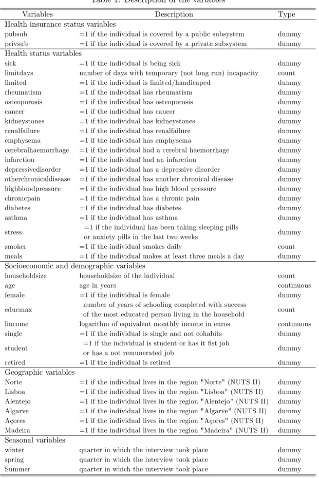
Table 1 presents the …nal covariates used in our analysis clustered into groups encompassing
health insurance status, socioeconomic characteristics, and health status. In addition, two further
groups were also included to control for geographic and seasonal e¤ects. We selected them among
the raw data available in the database10 according to their in‡uence on medical care consumption,
taking into account the Grossman’s health capital model of demand for health (1972) as well
as the results of similar empirical studies (Cameron et al. 1988, Pohlmeier and Ulrich 1995,
Vera-Hernández 1999, Deb and Trivedi 2002 and Lourenço 2007). Grossman (1972) constructed
a model in which health demand results from an investment on durable capital stock in order to
produce future healthy time. According to microeconomic theory, the main factors taken into
account in the estimation of a demand curve should be the budget constraint and individual
preferences. Although economists have di¢culties in understanding consumer incentives for
health care, it is possible to …nd several channels through which the selected variables a¤ect the
number of doctor visits. The problem is that the quantity of visits is only partially a result of
consumer incentives because the doctors play an important role in medical choices. Depending
on the kind of patient, we can have extreme cases of complete delegation of decisionmaking to
the doctor. For this reason moral hazard e¤ects are also relevant on the doctors side (demand
inducement).
1 0Some information was excluded from the analysis, particularly the questions reported only by part of the
Table 1: Description of the variables
Variables Description Type
Health insurance status variables
pubsub =1 if the individual is covered by a public subsystem dummy
privsub =1 if the individual is covered by a private subsystem dummy
Health status variables
sick =1 if the individual is being sick dummy
limitdays number of days with temporary (not long run) incapacity count
limited =1 if the individual is limited/handicaped dummy
rheumatism =1 if the individual has rheumatism dummy
osteoporosis =1 if the individual has osteoporosis dummy
cancer =1 if the individual has cancer dummy
kidneystones =1 if the individual has kidneystones dummy
renalfailure =1 if the individual has renalfailure dummy
emphysema =1 if the individual has emphysema dummy
cerebralhaemorrhage =1 if the individual had a cerebral haemorrhage dummy
infarction =1 if the individual had an infarction dummy
depressivedisorder =1 if the individual has a depressive disorder dummy
otherchronicaldisease =1 if the individual has another chronical disease dummy
highbloodpressure =1 if the individual has high blood pressure dummy
chronicpain =1 if the individual has a chronic pain dummy
diabetes =1 if the individual has diabetes dummy
asthma =1 if the individual has asthma dummy
stress =1 if the individual has been taking sleeping pills
or anxiety pills in the last two weeks dummy
smoker =1 if the individual smokes daily count
meals =1 if the individual makes at least three meals a day dummy
Socioeconomic and demographic variables
householdsize householdsize of the individual count
age age in years continuous
female =1 if the individual is female dummy
educmax number of years of schooling completed with success
of the most educated person living in the household count
lincome logarithm of equivalent monthly income in euros continuous
single =1 if the individual is single and not cohabits dummy
student =1 if the individual is student or has it …st job
or has a not remunerated job dummy
retired =1 if the individual is retired dummy
Geographic variables
Norte =1 if the individual lives in the region "Norte" (NUTS II) dummy
Lisboa =1 if the individual lives in the region "Lisboa" (NUTS II) dummy
Alentejo =1 if the individual lives in the region "Alentejo" (NUTS II) dummy
Algarve =1 if the individual lives in the region "Algarve" (NUTS II) dummy
Açores =1 if the individual lives in the region "Açores" (NUTS II) dummy
Madeira =1 if the individual lives in the region "Madeira" (NUTS II) dummy
Seasonal variables
winter quarter in which the interview took place dummy
spring quarter in which the interview took place dummy
The underlying health status and the socioeconomic characteristics play a major role in
the preferences formation. Health status also in‡uences the constraints limiting the pursuit of
preferences since illness events usually imply a loss of income (although sometimes partially
o¤set by sickness bene…ts). In the PHS, health status is only indirectly captured through some
questions that re‡ect details about current medical conditions (e.g. sickness episodes and limited
days) and the presence of chronic diseases or pains (e.g. rheumatism, cancer and diabetes).
Besides including such variables, the consumption of sleeping and anxiety pills is used as a
proxy to the level of exposure to stress, as well as some other regressors related to attitudes
with a potential impact on health, like the number of meals and a dummy variable reporting
a smoker/non-smoker individual. Despite being crude measures, these last regressors allow to
capture some remaining health aspects and some unobserved in‡uences.11;12
The variables representing demographic and socioeconomic features of the interviewed can
in‡uence simultaneously the decision to seek health care directly and indirectly through their
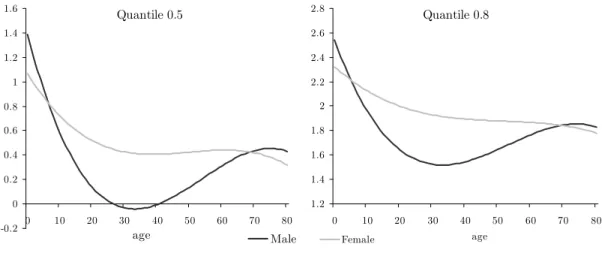
impact on health care status. This is particularly evident when analysing the covariate age.
According to Grossman (1972), age captures the depreciation of health capital which in‡uences
the health status and is an important factor in‡uencing individual preferences. It is expected
that the rate of depreciation increases as the individual gets older, at least after some point of
the life cycle, making the healthy times decrease. As a consequence, the demand for health care
is expected to increase over the life cycle. At the same time, age is an extra variable that can
be considered as a health status proxy since older individuals are, on average, less healthy and
less e¢cient in producing health. We chose to control for age through a nonlinear relationship
and by including variables that allow an assessment of its e¤ect by gender type.
Amongst the socioeconomic covariates, a gender dummy was included because it is believed to
in‡uence the rate at which the health stock depreciates and the e¢ciency in producing healthy
times. It is expected that health depends on biological di¤erences between man and women
1 1Winkelmann (2004) and Winkelmann (2006) also include individual subjective self-assessment of health status.
PHS provides that information (with the question "How well do you perceive your own health at the present time?", with responses "very good", "good", "fair", "poor" and "very poor") but we excluded its use. These variables are likely to create an endogeneity problem: the self-understanding of the health status in‡uences the consumption of medical care but it is also in‡uenced by consumption since the assessment is made after visiting the doctor. As suggested by Windweijer and Santos-Silva (1997), we control for this subjective health evaluation by including long-term determinants of health (smoking and eating habits).
1 2Engagement in sports activities is an alternative proxy for good health but was only available for a small part
through innate features, life styles and di¤erent attitudes towards health risk. Accordingly,
we also control for the marital status with the inclusion of the covariate single. Besides the
arguments of di¤erent life styles and attitudes toward risk, it is our understanding that some
decisions when taken by more than one person bene…t from advice and more information, which
should in‡uence health status and e¢ciency in producing healthy times.13
To control for educational level, it was de…ned a variable with the number of schooling years
of the most educated person living in the household. It is expected that more educated people
are more productive in the market as well as in the household, therefore even if they seek for
more health they need less medical care. On the other hand, di¤erent educational levels are
associated with di¤erent opportunity costs and attitudes towards risk. This particular indicator
was chosen, as an alternative to the usual number of the schooling years of each individual,
because we believe that the decision about the number of visits to a doctor is at least partially
a decision of the household and again bene…ting from a better level of information.
The variables student and retired capture occupational status which may explain some
dif-ferences in the depreciation rate. It is expected that a person who does not work, presents lower
opportunity costs (in terms both of time and income) of visiting a doctor, than an individual with
a regular job. Further, since hours of market or non-market can have di¤erent values and the
stock of health determines the total amount of time to spend producing earnings and
commodi-ties, it is expected that more active individuals invest more in health capital. These particular
variables can capture some income and age e¤ects (traditionally students are the youngest in the
database and the retired the oldest).
Another variable included in the model is the monthly equivalent income. In the dataset
income is measured by a ordinal variable with ten thresholds that indicate the category of the
disposable net household income in the month prior to the interview (including wages, pensions,
and all sort of social security bene…ts). A common way to control for income e¤ects is including
in the model a set of dummy variables, one for each category. We chose to construct a monthly
income variable following the adjustment proposed by Pereira (1995) by interpolating grouped
1 3Most of the studies include a slightly di¤erent variable that assumes one if the person is married instead of
data, and in a second stage taking into account di¤erences in household characteristics.14;15
According to Grossman (1972) there are reasons to believe that medical utilization increase with
income: "The higher a person’s wage rate, the greater the value to him of an increase in healthy
time". The idea is that the cost of being ill is higher. A converse argument is that the opportunity
cost of going to the doctor is higher for higher wages. In addition to this, income also represents
the ability to pay, as a proxy of wealth.
The variables Norte, Lisboa,Alentejo, Algarve,Açores and Madeira represent the region of
residence and were included to control for possible behavioural di¤erences in the demand and
supply of health care services.16 The regions encompass wide areas but nevertheless, when we
compare them in terms of wealth or educational indicators we obtain huge di¤erences, which
could justi…e di¤erent behaviours on seeking for health care services (not totally captured at
the individual level). Apart from this argument, the main reason to include these variables
is because they proxy di¤erent access to medical care supply, since some regional services are
di¤erently organized. Note that in the continent, the …ve regions correspond to the …ve regional
health administrations, and in the autonomous regions there are two di¤erent regional health
services.17
To control for the period of the year in which the interview took place we included the
regressorsspring,summer, andwinter (autumn being omitted). This is important because there
may be some seasonal di¤erences in individuals health status.
Finally, we use the health insurance dummy variables to distinguish between control and
treatment groups. In this case we have a control group "NHS" composed by individuals with
only the default health system, and two di¤erent treatments "Public subsystems" and "Private
subsystems".18 We managed to do it by dividing the observations according to the type of health
insurance, in particular by considering three mutually exclusive groups that is compared with
1 4To perform the interpolation of grouped data, we assumed that the midpoint of the interval at which the
family belongs is the income of the household. It was necessary to assume a value of 2500 for the last, open ended, income bracket (we test the robustness to this value by considering other values). To make the normalization to account for the family characteristics we used the square root scale, through dividing the household income by the square root of household size.
1 5Note that it is not necessary neither to de‡ate this variable nor to make it comparable across countries. 1 6In accordance with NUT II classi…cation (o¢cial territorial nomenclature for statistical analysis), Portugal is
divided into seven regions. The survey includes data for all of them. Therefore, we use six dummies.
1 7Lourenço (2007) used a dummy variable for a rural versus urban location that could not be included on the
basis of the data from the fourth PHIS. The di¤erence, however, is partially controlled for the region variables since they have di¤erent proportions of rural and urban areas (e.g. Lisboa andAlentejo).
the control group. according to their health care coverage: only the NHS, the NHS plus a public
subsystem or the NHS plus a private subsystem.19 These variables are of particular importance
since the main goal of this work is to assess how a patient´s use of medical consultations is
a¤ected by types of health insurance. From a theoretical point of view, insurance is a price proxy,
therefore, these variables together with income determine the budget constraint. Note that the
di¤erences between health systems as regards costs to bene…ciaries (as co-payments and
non-reimbursements) work as direct prices and mechanisms to control for its use, and delivery systems
are indirect costs of access. When compared to the NHS, the subsystems provide more bene…ts to
their bene…ciaries by decreasing the price-per-service faced by patients, which whenever demand
is elastic, increases their health care demand (Barros et al. 2008).20 The estimation of this moral
hazard e¤ect is particularly di¢cult in a context of adverse selection as it leads to endogeneity of
the treatment variables and results in an overestimation of its impact. As noted by Barros et al.
(2008) the exogeneity of both types of coverage removes the need for using instrumental-variables
estimation (for more details see Section 4.3).
3.3 An exploratory analysis of the data
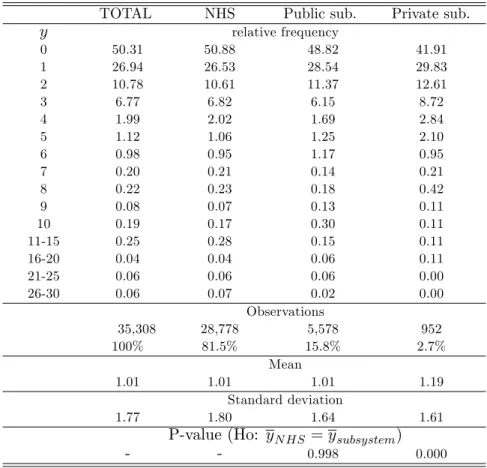
Table 2 presents the empirical distribution of the dependent variable (y) and some statistics.
As the table shows, the majority of observations are of the NHS group, followed by the public
subsystem. The dependent variable used is a count variable (non-negative integer valued count
y= 0;1;2; : : :) with a large proportion of zeros (half of the sample) as well as a long right tail of
individuals who make heavy use of health care. These features make the estimation particularly
di¢cult since it will be necessary to use ‡exible models that accommodate them. For the whole
sample, the average number of consultations is 1.01 and the average number of visits to those
that have at least one visit is 2.04. Moreover, the unconditional variance is more than three times
the unconditional mean.21 When we analyse the average number of visits to a doctor by health
insurance systems, it is possible to observe that private subsystems bene…ciaries are higher users
than NHS and public subsystems groups. Indeed, a mean comparison t-test indicates that the
unconditional probability does not di¤er across NHS and public subsystems but di¤er when one
compares NHS with private subsystems.
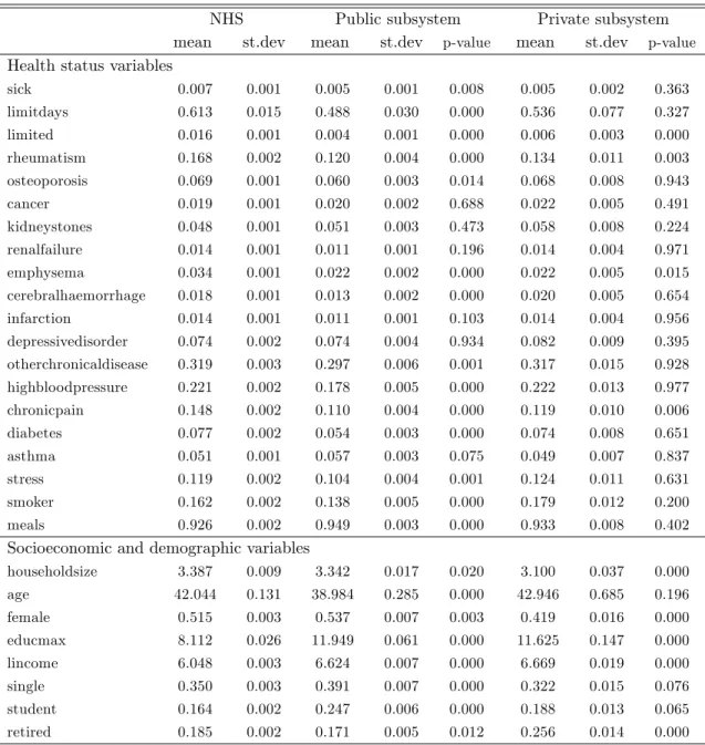
Table 3 presents the descriptive statistics of the explanatory variables by health insurance
type. The mean comparison t-test indicates that most of the di¤erences between the three types
are signi…cant, specially when one looks to socioeconomic pre-determined variables. The NHS
group has relatively less years of education and less income. On its turn, public subsystems
bene…ciaries are younger (on average about 4 years less than the other groups), have a greater
proportion of students and singles and a smaller share of retired persons. The private subsystems
group has less women and a smaller household size. As regards the health status distributions
of the three groups, it is possible to conclude that the major di¤erences are found between the
public subsystem and the NHS. The public employees seem to be the healthier, in particular
when we analyse some variables related to physical limitations (limited days andlimited) and to
the presence of chronic diseases and pains.
Table 2: Empirical distribution of the dependent variable
TOTAL NHS Public sub. Private sub.
y relative frequency
0 50.31 50.88 48.82 41.91
1 26.94 26.53 28.54 29.83
2 10.78 10.61 11.37 12.61
3 6.77 6.82 6.15 8.72
4 1.99 2.02 1.69 2.84
5 1.12 1.06 1.25 2.10
6 0.98 0.95 1.17 0.95
7 0.20 0.21 0.14 0.21
8 0.22 0.23 0.18 0.42
9 0.08 0.07 0.13 0.11
10 0.19 0.17 0.30 0.11
11-15 0.25 0.28 0.15 0.11
16-20 0.04 0.04 0.06 0.11
21-25 0.06 0.06 0.06 0.00
26-30 0.06 0.07 0.02 0.00
Observations
35,308 28,778 5,578 952
100% 81.5% 15.8% 2.7%
Mean
1.01 1.01 1.01 1.19
Standard deviation
1.77 1.80 1.64 1.61
P-value (Ho: yN HS =ysubsystem)
Table 3: Descriptive statistics by health insurance system
NHS Public subsystem Private subsystem
mean st.dev mean st.dev p-value mean st.dev p-value
Health status variables
sick 0.007 0.001 0.005 0.001 0.008 0.005 0.002 0.363
limitdays 0.613 0.015 0.488 0.030 0.000 0.536 0.077 0.327
limited 0.016 0.001 0.004 0.001 0.000 0.006 0.003 0.000
rheumatism 0.168 0.002 0.120 0.004 0.000 0.134 0.011 0.003
osteoporosis 0.069 0.001 0.060 0.003 0.014 0.068 0.008 0.943
cancer 0.019 0.001 0.020 0.002 0.688 0.022 0.005 0.491
kidneystones 0.048 0.001 0.051 0.003 0.473 0.058 0.008 0.224
renalfailure 0.014 0.001 0.011 0.001 0.196 0.014 0.004 0.971
emphysema 0.034 0.001 0.022 0.002 0.000 0.022 0.005 0.015
cerebralhaemorrhage 0.018 0.001 0.013 0.002 0.000 0.020 0.005 0.654
infarction 0.014 0.001 0.011 0.001 0.103 0.014 0.004 0.956
depressivedisorder 0.074 0.002 0.074 0.004 0.934 0.082 0.009 0.395
otherchronicaldisease 0.319 0.003 0.297 0.006 0.001 0.317 0.015 0.928
highbloodpressure 0.221 0.002 0.178 0.005 0.000 0.222 0.013 0.977
chronicpain 0.148 0.002 0.110 0.004 0.000 0.119 0.010 0.006
diabetes 0.077 0.002 0.054 0.003 0.000 0.074 0.008 0.651
asthma 0.051 0.001 0.057 0.003 0.075 0.049 0.007 0.837
stress 0.119 0.002 0.104 0.004 0.001 0.124 0.011 0.631
smoker 0.162 0.002 0.138 0.005 0.000 0.179 0.012 0.200
meals 0.926 0.002 0.949 0.003 0.000 0.933 0.008 0.402
Socioeconomic and demographic variables
householdsize 3.387 0.009 3.342 0.017 0.020 3.100 0.037 0.000
age 42.044 0.131 38.984 0.285 0.000 42.946 0.685 0.196
female 0.515 0.003 0.537 0.007 0.003 0.419 0.016 0.000
educmax 8.112 0.026 11.949 0.061 0.000 11.625 0.147 0.000
lincome 6.048 0.003 6.624 0.007 0.000 6.669 0.019 0.000
single 0.350 0.003 0.391 0.007 0.000 0.322 0.015 0.076
student 0.164 0.002 0.247 0.006 0.000 0.188 0.013 0.065
retired 0.185 0.002 0.171 0.005 0.012 0.256 0.014 0.000
Note: The p-value indicates the probability of the mean of each variable does not signi…cantly di¤er across insurance types. The test is performed as a two-sample mean-comparison test (unpaired). For the comparison between the NHS and the Public subsystem we considered H0: yN HS = yP ublic subsystem; and for the comparison between the NHS and the Private subsystem we considered H0: yN HS =yPrivate subsystem. Geographic and seasonal statistics (and p-values) not reported. Available from the authors upon request.
Moreover, frequent health problems (e.g. high blood pressure, diabetes and stress) are
rel-atively more common in the NHS and private subsystem groups. This feature can be partially
related with the age, which is lower among the public subsystems group. Additionally, it is worth
highlighting that public employees seem to be less exposed to stress and that the indicators
The regional distribution of the groups is also unequal in the full sample: most of the NHS
individuals are located in the North; the public employees are concentrated in Lisbon, Alentejo
and Azores; and the private subsystem group has relatively more bene…ciaries in the regions of
Lisbon and Algarve.
These sample di¤erences suggest that a more complete account for them is required, so that
an appropriate comparison of health care demand across groups can be made.
4
Econometric framework
Econometrics of count data has its own modelling strategies in which discreteness and
non-negativity are taken into account. Moreover, in thecount world it is common that features other
than location depend on the covariates, making the estimation of the conditional expectation
poorer in the sense that provides very little information about the impact of the regressors on the
outcome of interest. In this context it is potentially interesting to study the e¤ect of regressors
not only on the mean but also on single outcomes and in the full distribution.
Within the vast literature on count data it is possible to …nd two general categories of methods
that allow a complete description of the conditional distribution of a count outcome. Following
the early work of Hausman, Hall, and Griliches (1984), several fully parametric probabilistic
models, like Poisson and negative binomial regressions, have been developed in order to describe
the e¤ect of the covariates on di¤erent points of a count variable. These regressions allow
infer-ences for all possible aspects of the outcome variable (including the computation of the marginal
probability e¤ects). However, to do it, they impose restrictive parametric assumptions on the
way the independent variables a¤ect the outcome variable. As a consequence, this approach
usu-ally face a lack of robustness, even when ‡exible models like the hurdle or latent class models are
applied. Given these limitations, it can be attractive to use non- or semiparametric techniques
that freely approximate the conditional distribution. This can be achieved with the estimation
of conditional quantile functions, a technique that has been applied in the context of continuous
regression for a long time (Koenker and Bassett 1978). Following the contributions of Manski
(1975), Manski (1985) and Horowitz (1992) regarding binary models, some e¤ort is being made
(2005) succeeded in applying the quantile framework to count data models. Since our main
aim is to assess the e¤ect of the subsystems on di¤erent parts of the outcome distribution
with-out imposing a probabilistic structure, the "Quantile for counts" regression model is a natural
choice.22
4.1 Quantile regression for counts
Lety be a count random variable and their -quantile de…ned as:
Qy( ) = min [ jP(y ) ] where 0< <1 (1)
The -quantile has the same discrete support asyand cannot be a continuous function of the
covariates (x). Machado and Santos-Silva (2005) suggested a procedure known as “jittering” to
arti…cially impose some degree of smoothness. The basic idea is to build a continuous auxiliary
variable (y ) whose quantiles have a one-to-one known relationship with the quantiles of the
count variable of interest. They is obtained by adding to the count variable a uniform random
variable independent of y and x:23
y =y+u where u unif orm[0;1) (2)
The continuity problem of the dependant variable is solved but the derivatives are not
contin-uous for integer values ofy . Machado and Santos-Silva (2005) proved that given some regularity
conditions, valid asymptotic inference is possible. Among those conditions, it is particularly
rel-evant the existence of at least one continuously distributed covariate. The standard quantile
regression is applied to a monotonic transformation ofy that ensures that the estimated
quan-tiles are non-negative and the transformation is linear in the parameters of a vector of regressors.
In order to implement the procedures, the authors suggest the following parametric
repre-2 repre-2In order to better understand its advantages (and disadvantages), Moreira (2008) compares the implications
drawn from the quantile regression approach with those from parametric count data models that have been used quite extensively in the analysis of health care.
2 3Machado and Santos-Silva (2005) showed that there is a little loss of generality in assuming that U is uniform.
sentation of the -quantile of y :
Qy ( jx) = + exp x0 ( ) ; 0< <1: (3)
The reason for adding to the right side is that y is bounded from below at due to
the way it is constructed. The exponential form is traditionally assumed in count data models.
We believe that this speci…cation provides a good parsimonious approximation to the unknown
conditional quantile functions. The linear transformation is speci…ed as:
QT(y ; )( jx) =x0 ( ); (4)
where T(y ; ) =f log(log("y) )forfory >y ;being"a small positive number (0< " < ).24
This is feasible because quantiles are equivariant to monotonic transformations and to
cen-soring from below up to the quantile of interest. The vector of covariates ( ) is obtained as
a solution to a standard quantile regression of a linear transformed variable by minimizing an
asymmetrically weighted sum of absolute errors
min
n X
i=1
T(y ; ) x0i where (v) =v[ I(v <0)]: (5)
Machado and Santos-Silva (2005) proved that although the quantile regression is not
di¤er-entiable everywhere, the estimator is consistent and asymptotically normal:
p
nhb( ) ( )i D!N(0; D 1AD 1) (6)
withA= (1 )E(XX0)and D=E[fT(X0 ( )jX)X0X], wherefT denotes the conditional
density ofT(y ; ) givenX.
Because "noise" has been arti…cially created for technical reasons, Machado and Santos-Silva
(2005) suggest a Monte Carlo procedure - an "average-jittering" - which consists in obtaining
an estimator that is the average ofm independent "jittering" samples with the same size. The
di¤erence between samples is the dependent variable y because it is created as the sum of
y (constant between samples) with m di¤erent draws of the uniform distribution. The main
advantage of this procedure is that the resulting estimator is more e¢cient than the one obtained
from a single draw and a misspeci…cation-robust estimator of the covariance matrix is available.
The importance of this procedure derives from the possibility of performing inferences on
the variable of interesty. Machado and Santos-Silva (2005) showed that marginal e¤ects of the
smoothed variable y are easily obtained and interpreted and that there is a correspondence
between the two quantile functions:
Qy( jx) =dQy ( jx) 1e, wheredae denotes the ceiling function (returns the smallest
inte-ger greater than, or equal to a).
Because of the monotone transformation ofy (T(y ; )), the relationship between coe¢cient
estimates b( ) and y and y is essentially non-linear, making it hard to interpret b( ) in terms
of y and y. It is possible to test the null hypothesis that a covariate has no e¤ect on Qy( jx)
because it is equivalent to test whether the variable has no impact on theQy ( jx). The problem
is when the variable is signi…cant in Qy ( jx). In such case it could be non signi…cant in the
conditional quantile ofy.25 This occurs because di¤erent quantiles ofy correspond to the same
quantiles of y. In fact, a change in xj will a¤ect Qy( jx) only if it is capable of changing the
integer part ofQy ( jx):Machado and Santos-Silva (2005) call this "magnifying glass e¤ect" of
Qy ( jx).
4.2 Empirical speci…cation: treatment e¤ects
Our empirical work presents two main di¤erences relative to general treatment e¤ects approaches.
Firstly, the study is about a potential reform, not a real one, as it is usually the case. We can
state our interest as to measure the potential impact of the elimination of double coverage
(par-ticularly the insurance plans provided to public employees) on the demand of health services, i.e.
the potential decrease in the demand for health services amongst the subsystems bene…ciaries
due to their double coverage. To proxy such impact we study the di¤erences in the consumption
of doctor consultations between NHS and public and private subsystems. Generally, the
estima-tion of the impact of a reform occurs after its implementaestima-tion and uses panel data comparing
the outcome before and after the reform (Winkelmann 2006). In that case, the typical
empir-2 5It is not possible to just look at
j, as it becomes necessary to evaluate case by case if a given magnitude inxj
induces changes in the -quantile ofy. Inference about the partial e¤ect of a particular variation of the regressor, given that all other variables remain …xed atexis made through the following expression:
ical strategies include pre-reform/post-reform di¤erences-in-di¤erences where one compares the
changes in the utilization between a¤ected and una¤ected sub-populations. A drawback in our
analysis relative to more general approaches is that we estimate the current impact (the impact
in 2005), which may change in case of di¤erent time paths between groups. But an advantage
is that we analyze not only the average e¤ect but also the impact on the whole outcome
distri-bution. With quantile regression we are able to see if the policy impact di¤ers depending of the
outcome on the realization of the dependent variable.
As laid out in the previous section, and now presented in a more speci…c way, the conditional
quantiles are de…ned as26
Qy ( jx) = + exp [ 0( ) + 1( )pubsubi+ 2( )privsubi+ ( )zi]; (7)
0 < <1 and i= 1; 2;:::; 35;308
where pubsubi and privsubi represent persons "treated" as belonging to the "public insurance
health subsystem" and "private insurance health subsystem", respectively. The vectorziincludes
all other characteristics that were controlled for in this regression. In addition to all independent
variables referred in section 4.2, we use a third order polynomial in age and a third order
poly-nomial inage crossed with the gender variable (age f emale). Note that it is absolutely crucial
in this analysis to assume ignorability of the treatment conditional on a set of covariates. The
alternative to assume ignorability and estimate treatment e¤ect with di¤erence in sample means
is obviously bad since, as we tested, there are huge di¤erences between control and treatment
groups across their baseline characteristics. Moreover, when selecting the variables we guarantee
that treated and untreated groups have a common support by using only observations in the
intersection of the domains.27 This procedure makes us exclude individuals with more than 80
years old and a variable related to unemployment status.
We discard a selection bias problem. The exogeneity of the treatments holds because it is
very implausible that individuals want to work as public employees or in companies with private
subsystems just to bene…t from this additional health insurance (Barros et al. 2008). Note
2 6The vector of coe¢cients is now ( ) = [
0( ); 1( ); 2( ); ( )] , being 0( ); 1( ); 2( )scalar and ( )a vector.
that they have an alternative since we are studying a country that provides universal coverage
through the NHS. Moreover, it is also unlikely that employers choose individuals on the basis of
unobservable variables related to their health or even household health. The only requirement is
that the potential employee (and not his household) is physically capable and has no infectious
disease which could be controlled through our set of pre-determined variables. Nevertheless, even
controlling for a large set of health status variables, this kind of procedure can still underestimate
1( ) and 2( ) if the subsystems bene…ciaries enjoy more or better treatment than the NHS
bene…ciaries. This is because over life, better health care would translate into a signi…cant
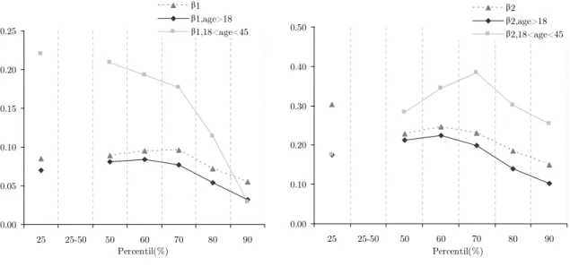
accumulation of health advantages not totally captured in zi. Following the advice of (Barros
et al. 2008), we will test this possibility restricting the analysis to young bene…ciaries who did
not yet had time to accumulate such advantages and compare the results with the larger sample.
Note that the coe¢cients 1( ) and 2( ) cannot be totally associated with moral hazard
behaviour but it is instead a joint e¤ect of moral hazard from the bene…ciaries and supply-induced
demand from the providers. The latter is more likely because doctors may require more tests in
order to justify more visits. According to (Barros et al. 2008), since the payments to subsystems
providers are relatively low, the magnitude of the e¤ect will be very small. Independently of
that, the important here is to capture how much the systems design increases the consumption
of resources related to consultations.
5
Results
The results were obtained from theqcount package of STATA (Miranda 2006) with some slight
adjustments. Regarding the number of jittered samples used to obtain the results, preliminary
experiments showed that the coe¢cients are not very sensitive to a particular sample of uniform
random variables used to jitter the data: with 1500 samples almost no changes were detected both
in coe¢cients and in standard deviations.28 The decision on which quantiles to compute took
into account the problem under analysis and the empirical distribution of the relevant outcome.
Since the marginal quantiles are zero for all 60:50, it becomes more interesting to compute
conditional quantiles on the upper tail of the distribution where the e¤ect of covariates changes
rapidly. Note that in the lower tail, a variation in the conditional quantiles of the arti…cial
outcome Qy ( jx) may be mostly due to the random noise that has been added. Therefore, we
expect to …nd quantiles more ‡at. Moreover, it is more interesting to look at the behaviour of
individuals who make heavy use of health care. In this scenario, and despite the fact that we
will still be presenting the …rst quartile, we will focus on quantiles above the median, computing
results for each decile after the median.
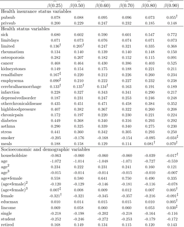
Table 4 presents the parameter estimates of the quantiles regressions (the corresponding
standard errors are shown in Table A1 of the Appendix). As we can see, quantile regression
does not restrict the way regressors a¤ect di¤erent regions of the distribution, allowing the
assessment of whether health insurance systems have signi…cant and variable impacts over the
di¤erent outcomes. The signs of the regressors do not switch across the di¤erent quantiles (except
for the dummysummer, whose e¤ect, albeit highly insigni…cant, is positive in the lower tail and
becomes negative in the upper quantiles).
Regarding the statistical signi…cance, all variables are signi…cant in at least one quantile. In
the group of health status regressors, the covariates that control for current medical conditions
are highly signi…cant as expected. Among the chronic diseases dummies, only the cerebral
haem-orrhage e¤ect is not signi…cant in quantiles above the 0:7y quantile. Concerning indicators
related to attitudes with impact on health status, we …nd that both the number of meals and
smoking habits are insigni…cant in the upper tail of the distribution. In the case of socioeconomic
characteristics, the household size, education and income e¤ects are signi…cant at the one per
cent level except for the last decile. Most of the variables related to the region of residence and
Table 4: Quantile regression results: coe¢cients
_
(0:25)
_
(0:50)
_
(0:60)
_
(0:70)
_
(0:80)
_
(0:90)
Health insurance status variables
pubsub 0.078 0.088 0.095 0.096 0.073 0.055y
privsub 0.200 0.229 0.247 0.232 0.185 0.148
Health status variables
sick 0.680 0.602 0.590 0.601 0.547 0.772
limitdays 0.071 0.073 0.076 0.074 0.071 0.073
limited 0.136y 0.205y 0.247 0.321 0.335 0.368
rheumatism 0.134 0.140 0.139 0.140 0.148 0.150
osteoporosis 0.282 0.207 0.182 0.152 0.115 0.091
cancer 0.468 0.464 0.430 0.386 0.403 0.525
kidneystones 0.149 0.154 0.175 0.188 0.221 0.211
renalfailure 0.167z 0.220 0.212 0.226 0.260 0.234
emphysema 0.090z 0.210 0.222 0.227 0.232 0.238
cerebralhaemorrhage 0.133y 0.135y 0.134y 0.163 0.191 0.189
infarction 0.228 0.327 0.343 0.341 0.290 0.217
depressivedisorder 0.187 0.231 0.247 0.253 0.246 0.248
otherchronicaldisease 0.435 0.451 0.471 0.458 0.384 0.352
highbloodpressure 0.407 0.382 0.367 0.322 0.260 0.208
chronicpain 0.172 0.197 0.220 0.230 0.221 0.224
diabetes 0.449 0.368 0.340 0.316 0.293 0.292
asthma 0.290 0.325 0.339 0.340 0.275 0.230
stress 0.441 0.360 0.342 0.305 0.293 0.250
smoker -0.205 -0.176 -0.168 -0.154 -0.095 -0.034z
meals 0.188 0.158 0.129 0.114 0.081y 0.070y
Socioeconomic and demographic variables
householdsize -0.063 -0.060 -0.060 -0.060 -0.039 -0.017y
age -1.072 -1.014 -1.048 -1.071 -0.727 -0.559
age2 0.234 0.222 0.231 0.241 0.160 0.121
age3 -0.015 -0.014 -0.014 -0.015 -0.010 -0.007
age female 0.558 0.580 0.641 0.750 0.490 0.335
(age female)2 -0.120 -0.129 -0.146 -0.181 -0.116 -0.078
(age female)3 0.007z 0.008 0.009 0.012 0.007 0.005y
female -0.321y -0.321 -0.345 -0.357 -0.216 -0.091z
educmax 0.010 0.014 0.015 0.015 0.010 0.005y
lincome 0.069 0.058 0.060 0.060 0.053 0.030z
single -0.218 -0.198 -0.202 -0.218 -0.164 -0.116
student -0.252 -0.246 -0.272 -0.253 -0.179 -0.172
retired 0.168 0.149 0.134 0.115 0.120 0.143
Notes: Coe¢cients marked withz and yare not signi…cant at a 5 and 1 per cent level, respectively. Standard errors can be found in the Table A1 of the Appendix. Geographic and seasonal controls not reported. Available from the authors upon request.
We now turn to the analysis of the e¤ects of the regressors beyond their statistical signi…cance.
The direct interpretation of Table 4 may suggest some misleading conclusions. Note that
_
( )is
should be made through Qy ( jx), which is not so easily computed due to its non-linearity as
well as to the fact that it is a function of quantile. Being non-linear, the parameter provides
an incomplete picture of the covariates’ e¤ects on the shape of the distribution. And being a
function of implies, for example, that a variable with the same estimated coe¢cient in all
quantiles will have a proportional e¤ect that varies with quantile. To take into account the
non-linearity, Table A2 of the Appendix presents estimates of the partial e¤ects computed setting
the continuous (and count) variables at the mean of the sample and the dummy variables equal to
zero (xe).29 Inference for the marginal e¤ect of a dummyxj given that all other variables remain
…xed atexis made throughQy ( jxe; xj = 1) Qy( jex; xj = 0) = exp( j( )) 1 [Qy ( jex) ]
and for a continuous variable xl is l( ) [Qy ( jex) ].30 To facilitate the comparison of the
e¤ects across the di¤erent models we also estimate the semi-elasticities of Qy ( jx) with respect
to the covariates. This is done by simply dividing the partial e¤ect by Qy ( jex). Table 5 shows
the results.
Using the quantile regression framework it may happen that a signi…cant coe¢cient of a
variable on y quantile may not a¤ect a particular conditional y quantile. But when it is
found that the y quantile depends on the covariate for several quantiles, then it should be
possible to detect a subpopulation for which the semi-elasticity ony quantile is di¤erent from
zero (Miranda 2008). For example, if we consider the median and compute the Qy (0:50jx=ex)
we obtain0:79as a consequenceQy(0:50jx=xe)is equal to zero consultations. When thetypical
individual (ex) changes to the public health plan, it is expected that an increase inQy to0:82, but
leaving Qy unchanged. Hence the marginal e¤ect of the public subsystem on the y quantile
is zero, even though it has a signi…cant positive e¤ect ony quantile. Conversely, if we utilize
the sixth decile theQy (0:60jx=xe) is equal to0:97and as a consequenceQy(0:60jx=xe) is also
equal to zero consultations. But now, a change from NHS to a public subsystem will increase
Qy to1:01 making Qy equal to one consultation.
2 9Thedefault individual is a healthy man with an average household size, educational level and income, not
single or retired, living in the Centre region of Portugal and interviewed in autumn. Also note that, the vectorex
is set with the dummiespubsub andprivsub equal zero, so thedefault individual has the NHS insurance plan (is from the control group).
3 0The marginal e¤ects of some covariates are calculated in a di¤erent way. This is the case of the income that
is computed as lincome( ) 1=income [Qy ( jex) ], the "age when male" that is set as [ age( ) + 2 age2( )
age+ age3( ) age2] [Qy ( jex) ], and the "age when female" that is [ age( ) + agexf emale( ) + 2( age2( ) +
Table 5: Quantile regression results: semi-elasticities
SE(0.25) SE(0.50) SE(0.60) SE(0.70) SE(0.80) SE(0.90) Health insurance status variables
pubsub 0.031 0.034 0.038 0.042 0.037 0.032
privsub 0.083 0.095 0.107 0.109 0.100 0.092
Health status variables
sick 0.367 0.304 0.307 0.343 0.359 0.668
limitdays 0.028 0.028 0.030 0.032 0.036 0.043
limited 0.055 0.084 0.107 0.158 0.196 0.256
rheumatism 0.054 0.055 0.057 0.063 0.078 0.093
osteoporosis 0.123 0.084 0.076 0.069 0.060 0.055
cancer 0.225 0.217 0.205 0.196 0.245 0.397
kidneystones 0.061 0.061 0.073 0.086 0.122 0.135
renalfailure 0.069 0.091 0.090 0.106 0.146 0.151
emphysema 0.035 0.086 0.095 0.106 0.129 0.154
cerebralhaemorrhage 0.054 0.053 0.055 0.074 0.104 0.120
infarction 0.131 0.142 0.156 0.169 0.166 0.139
depressivedisorder 0.078 0.096 0.107 0.120 0.137 0.161
otherchronicaldisease 0.205 0.210 0.230 0.242 0.231 0.242
highbloodpressure 0.189 0.171 0.169 0.158 0.146 0.133
chronicpain 0.071 0.080 0.094 0.108 0.122 0.144
diabetes 0.214 0.164 0.154 0.155 0.168 0.195
asthma 0.127 0.141 0.154 0.169 0.156 0.148
stress 0.209 0.159 0.156 0.149 0.168 0.163
smoker -0.070 -0.060 -0.059 -0.059 -0.044 -0.019
meals 0.078 0.063 0.052 0.050 0.042 0.042
Socioeconomic and demographic variables
householdsize -0.024 -0.022 -0.023 -0.025 -0.019 -0.010
age when male 0.005 0.004 0.005 0.006 0.004 0.003
age when female 0.001 0.000 0.000 -0.001 -0.001 -0.001
female 0.184 0.178 0.200 0.243 0.195 0.190
educmax 0.004 0.005 0.006 0.006 0.005 0.003
income 0.004 0.003 0.004 0.004 0.004 0.003
single -0.074 -0.066 -0.070 -0.082 -0.075 -0.063
student -0.084 -0.080 -0.091 -0.093 -0.081 -0.091
retired 0.069 0.059 0.055 0.051 0.063 0.088
Notes: Semi-elasticiies are calculated for a vectorxecontaining the mean value of the continuous (and count) variables and zeros for the dummy variables. The type of the covariates is presented in Table 2 and the mean values can be obtained from Table 3. Geographic and seasonal controls not reported. Available from the authors upon request.
Starting with the analysis of insurance treatment e¤ects, it is visible that they do not change
a lot across the estimated quantiles, but it is possible to …nd a pattern: both public and private
subsystems have an increasing positive e¤ect on the number of doctor visits until the 0:60y
0:70y quantiles and a decreasing positive e¤ect thereafter (Table 5). The similarities between the
since it remains almost unchanged. In fact, the e¤ect of private insurance plans is between 2:6
and 2:9times higher than the impact of those of public employees. Therefore, health insurance
double coverage does lead to further demand of health care (visits). The origin of double coverage
is also quite important, as private subsystems double coverage induces much more demand than
public subsystems double coverage.
To better understand the e¤ect of health subsystems on the demand for health care we used
the point estimates to predict the y quantile (note that here we use the relevant outcome)
for each observation in a simulation exercise in which all variables are set equal to their actual
values, except the health insurance status. About this one three possibilities are considered: no
treatment, public subsystem or private subsystem. The results measured by relative frequencies
are presented in Table 6. Given that half of the sample has zero visits, it is not surprising that
the …rst conditional quartile is zero for almost all observations. When we compare the estimates
from di¤erent quantiles, we have the perception that the distribution changes di¤erently across
the health insurance plans. For example, the proportion of individuals with a predicted quantile
of zero or one consultation is always lower with the treatment (either public or private) than with
NHS, but these relative e¤ects change with the quantile. More particularly, the proportion
of NHS individuals is 91:0, 70:7 and 23:4 per cent for the 0:50y , 0:75y , 0:90y quantile,
respectively, while with the "public subsystem" the proportion is 89:6, 66:4 and 19:5 per cent
for the 0:50y , 0:75y ,0:90y quantile, respectively. This means that holding double coverage
causes a decreasing path in the di¤erence of proportion of individuals with a certain (increasing)
number of visits that is steeper from the 0:50y quantile to the 0:75y quantile than from the
Table 6: Frequencies of estimated quantiles for the number of visits to a doctor
0 1 2 3 4 5 6 7 8 9 >10
NHS
_
Qy(25jx) 89:4 8:3 1:4 0:4 0:2 0:1 0:1 0:0 0:0 0:0 0:0 _
Qy(50jx) 58:2 32:8 5:5 1:7 0:7 0:4 0:2 0:1 0:1 0:1 0:2
_
Qy(75jx) 1:3 69:3 17:9 5:6 2:5 1:1 0:7 0:5 0:2 0:2 0:7 _
Qy(90jx) 0:0 23:4 46:3 15:1 6:2 3:1 1:8 1:1 0:7 0:5 1:8
Public subsystem
_
Qy(25jx) 87:9 9:4 1:6 0:5 0:3 0:1 0:1 0:0 0:0 0:0 0:0 _
Qy(50jx) 54:0 35:7 6:3 2:0 0:9 0:5 0:2 0:2 0:1 0:1 0:2 _
Qy(75jx) 0:7 65:7 20:1 6:5 2:9 1:4 0:8 0:5 0:3 0:2 0:8
_
Qy(90jx) 0:0 19:5 47:2 16:6 6:7 3:5 1:9 1:2 0:8 0:6 2:0
Private subsystem
_
Qy(25jx) 83:6 12:3 2:4 0:8 0:3 0:2 0:1 0:1 0:1 0:1 0:1
_
Qy(50jx) 46:8 40:3 7:5 2:6 1:2 0:6 0:3 0:2 0:1 0:1 0:3 _
Qy(75jx) 0:2 60:0 23:4 7:6 3:6 1:8 0:9 0:7 0:5 0:3 1:0 _
Qy(90jx) 0:0 13:2 47:7 19:5 7:7 4:0 2:3 1:5 1:0 0:7 2:4 Notes: Estimates are based on a simulation exercise that start by predicting the y quantile for all 35,308 individuals setting all control variables in their actual values except the health insurance status, which is set in the three possible cases. After that, they quantiles are computed applying Qy( jx) =dQy ( jx) eand tabulated in their possible values.
Regarding the e¤ects of health status variables as a whole, it is visible that most of the
regressors have a positive e¤ect that increases with . Being sick seems to be especially important
to determine whether or not the individual visits a doctor but, taking into consideration the
results of the last decile, it is much more important in explaining the subsequent visits. The
same kind of behaviour is observed for the handicapped e¤ect, since for the …rst quantiles it is
not signi…cant whereas for higher levels of consumption it becomes a very important explanatory
variable. In the case of the sickness e¤ect this does not happen, which can be explained by the fact
that only in the 0:90y quantile the impact is substantial whereas the variable limited becomes
gradually more relevant. Amongst the chronic diseases we found evidence of a positive increasing
e¤ect along the estimated quantiles, except for the dummy osteoporosis that has a decreasing
impact, while infarction, otherchronicaldisease, highbloodpressure, diabetes and asthma have a
constant e¤ect in the di¤erent parts of the distribution. The proxy for the level of exposure to