Stability indicators in network reconstruction.

(1)

Stability Indicators in Network Reconstruction

Michele Filosi1,2., Roberto Visintainer1., Samantha Riccadonna3, Giuseppe Jurman1*, Cesare Furlanello1 1MPBA/Center for Information and Communication Technology, Fondazione Bruno Kessler, Trento, Italy,2CIBIO, University of Trento, Trento, Italy,3Department of Computational Biology, Research and Innovation Centre, Fondazione Edmund Mach (FEM), San Michele all’Adige, Italy

Abstract

The number of available algorithms to infer a biological network from a dataset of high-throughput measurements is overwhelming and keeps growing. However, evaluating their performance is unfeasible unless a ‘gold standard’ is available to measure how close the reconstructed network is to the ground truth. One measure of this is the stability of these predictions to data resampling approaches. We introduce NetSI, a family of Network Stability Indicators, to assess quantitatively the stability of a reconstructed network in terms of inference variability due to data subsampling. In order to evaluate network stability, the main NetSI methods use a global/local network metric in combination with a resampling (bootstrap or cross-validation) procedure. In addition, we provide two normalized variability scores over data resampling to measure edge weight stability and node degree stability, and then introduce a stability ranking for edges and nodes. A complete implementation of the NetSI indicators, including the Hamming-Ipsen-Mikhailov (HIM) network distance adopted in this paper is available with the R packagenettools. We demonstrate the use of the NetSI family by measuring network stability on four datasets against alternative network reconstruction methods. First, the effect of sample size on stability of inferred networks is studied in a gold standard framework on yeast-like data from the Gene Net Weaver simulator. We also consider the impact of varying modularity on a set of structurally different networks (50 nodes, from 2 to 10 modules), and then of complex feature covariance structure, showing the different behaviours of standard reconstruction methods based on Pearson correlation, Maximum Information Coefficient (MIC) and False Discovery Rate (FDR) strategy. Finally, we demonstrate a strong combined effect of different reconstruction methods and phenotype subgroups on a hepatocellular carcinoma miRNA microarray dataset (240 subjects), and we validate the analysis on a second dataset (166 subjects) with good reproducibility.

Citation:Filosi M, Visintainer R, Riccadonna S, Jurman G, Furlanello C (2014) Stability Indicators in Network Reconstruction. PLoS ONE 9(2): e89815. doi:10.1371/ journal.pone.0089815

Editor:Alberto de la Fuente, Leibniz-Institute for Farm Animal Biology (FBN), Germany ReceivedAugust 26, 2013;AcceptedJanuary 27, 2014;PublishedFebruary 27, 2014

Copyright:ß2014 Filosi et al. This is an open-access article distributed under the terms of the Creative Commons Attribution License, which permits unrestricted use, distribution, and reproduction in any medium, provided the original author and source are credited.

Funding:The authors acknowledge funding by Fondazione Bruno Kessler. The funders had no role in study design, data collection and analysis, decision to publish, or preparation of the manuscript.

Competing Interests:The authors have declared that no competing interests exist. * E-mail: jurman@fbk.eu

.These authors contributed equally to this work.

Introduction

The problem of inferring a biological network structure given a set of high-throughput measurements,e.g.gene expression arrays, has been addressed by a large number of different methods published in the last fifteen years (see [1,2] for two recent comparative reviews). Solutions range from general purpose algorithms (such as correlation [3] or relevance networks [4]) to methods tailoredad hoc for specific data types. Recent examples include SeqSpider [5] for Next Generation Sequencing data, or Sparsity-aware Maximum Likelihood [6] for cis-expression quan-titative trait loci (cis-eQTL).

However, network reconstruction is an underdetermined problem, since the number of interactions is significantly larger than the number of independent measurements [7]. Thus, all algorithms must aim to find a compromise between reconstruction accuracy and feasibility: simplifications inevitably detract from the precision of the final outcome by including a relevant number of false positive links [8], which should be discarded e.g., by identifying and removing unwanted indirect relations [9]. More-over, inference accuracy is strongly dependent on the assumptions used to choose the best hypothetical model of experimental observations [10].

These issues make the inference problem ‘‘a daunting task’’ [11] not only in terms of devising an effective algorithm, but also in terms of quantitatively interpreting the results obtained. In general, reconstruction accuracy is far from optimal in many situations and several pitfalls may occur [12], related to both the methods and the data [13]. In extreme cases, many link predictions are statistically equivalent to random guesses [14]. In particular, it is now widely acknowledged that the size and quality of the data play a critical role in the inference process [15-18]. All these considerations support the opinion that network reconstruc-tion should still be regarded as an unsolved problem [19].

(2)

standard is available for a given problem, there is no chance to evaluate algorithm accuracy. In such cases we can consider stability as a rule of thumb for judging the reliability of the resulting network. Obviously, the performance of a network reconstruction algorithm and the stability/reliability of the resulting network inferred from a specific dataset are two distinct and equally crucial aspects of the network inference process. The

best way to optimize both aspects would be to adopt only network reconstruction algorithms with well characterized performance,

i.e.,evaluated in cases where the ground truth is known, and with stability always checked on specific data. It is also worthwhile noting that the evaluation of inference stability is not related to the (chemical or physical) ‘‘stability’’ of the represented process. Figure 1. HIM distance: contribution of H and IM.(A) An example on three 5-node networks mutually differing by two links. (B) An example on networkG4, as defined in SubsectionStability is modularity invariant.Gred: networkG4without the four red links.Ggreen: networkG4without green links.Gblue: networkG4without blue links. (C) The mutual differences between the pairs of networks in (A),(NA,NB)and(NA,NC). (D)(G4,Gred), (G4,Ggreen),(G4,Gblue). In both cases they have the same Hamming distance but different spectral structure, thus resulting in different Ipsen-Mikhailov distances.

doi:10.1371/journal.pone.0089815.g001

Figure 2. An example of HIM distance.Representation of the HIM distance in the Ipsen-Mikhailov (IM axis) and Hamming (H axis) distance space between networks A versus B, E and F, where E is the empty network and F is the fully connected one.

(3)

We propose to tackle the stability issue by quantifying inference variability with respect to data perturbation, and, in particular, data subsampling. If a portion of data is randomly removed before inferring the network, the resulting graph is likely to be different from the one reconstructed from the whole dataset and, in general, different subsets of data would give rise to different networks. Thus, in the spirit of applying reproducibility principles to this

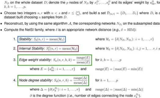
field, one has to accept the compromise that the inferred/non inferred links are just an estimation, lying within a reasonable probability interval. Here we introduce the Network Stability Indicators (NetSI) family, a set of four indicators allowing the researcher to quantitatively evaluate the reproducibility of the reconstruction process. We propose to quantitatively assess, for a given ratio of removed data and for a given amount of (bootstrap Figure 3. Definition of the NetSI family.

Figure 4. Graphical description of the pipeline in Fig. 3.Using the inference algorithmA, the networkNDis first reconstructed from the whole datasetDwithssamples andpfeatures (nodes). Given two integersn,r, a set ofrdatasetsDiis generated by choosing for eachia subset ofn samples fromD, and the corresponding networksNDi are inferred byA. Finally, the four indicatorsSd(n,r),S

I

d(n,r),Sw(n,r,h,k)andSd(n,r,h)are computed according to their definition.

(4)

[25] or cross-validation) resampling, the mutual distances among all inferred networks and their distances to the network generated by the whole dataset, with the idea that, the smaller the average distance, the more stable the inferred network. Similarly, we propose two indicators for the distribution of variability of the link weight and node degree across the generated networks, providing a ranked list of the most stable links and nodes, the least variable

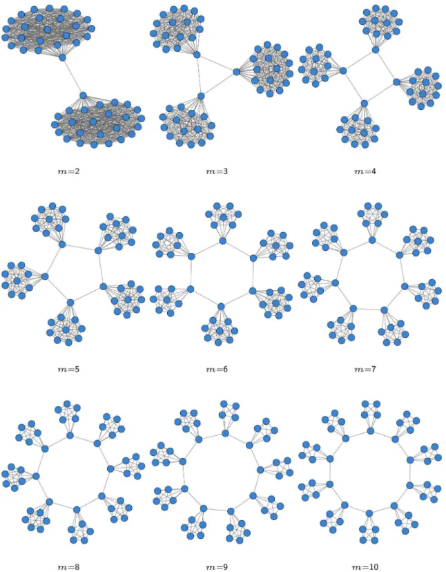
being the top ranked. The described framework for evaluating the stability of the whole network obviously relies on a network distance, but it is independent from the chosen metric. As network distance we use the Hamming-Ipsen-Mikhailov (HIM) distance [26], or its components for demonstration purposes, because it represents a good compromise between local (link-based) and global (structure-based) measures of network comparison. Figure 5. Synthetic network withmmodules, wheremranges from 2 to 10 from top left to bottom right.

(5)

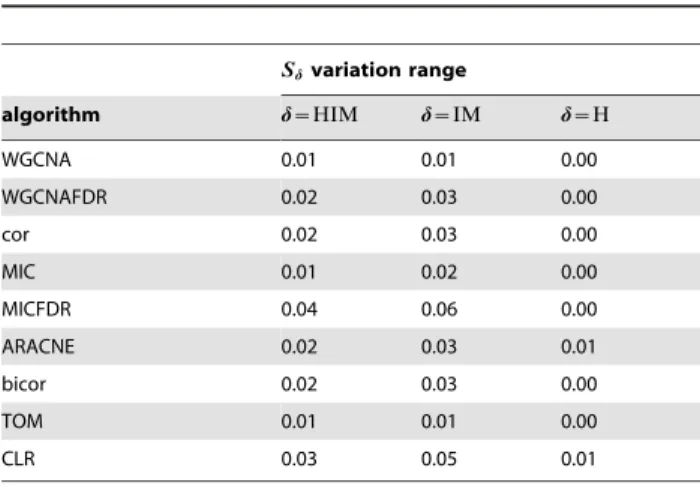
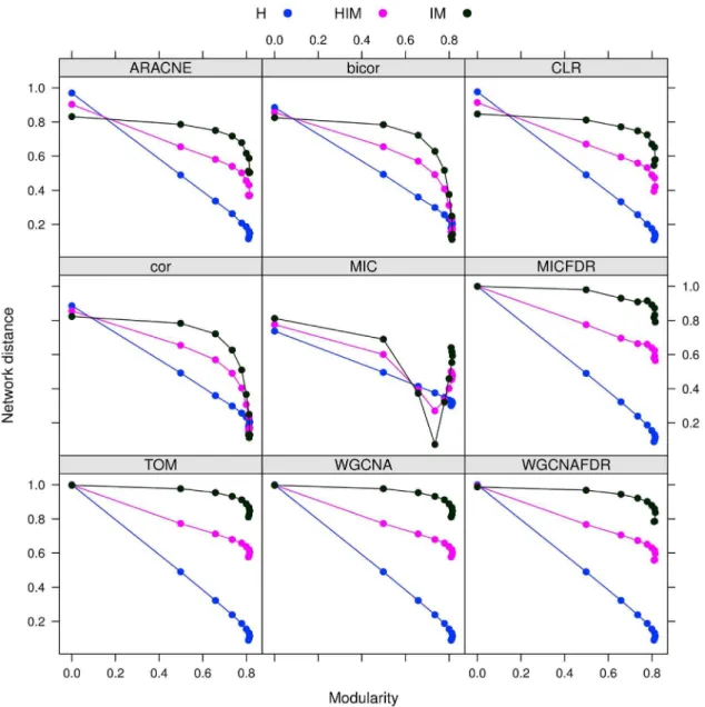
Figure 6.Gmnetworks: Stability of synthetic networks for different modularity levels. doi:10.1371/journal.pone.0089815.g006

Table 2.Gmnetworks: range ofSdfor different

reconstruction algorithms andd~fHIM,H,IMg.

Sdvariation range

algorithm d~_HIM d~_IM d~_H

WGCNA 0.01 0.01 0.00

WGCNAFDR 0.02 0.03 0.00

cor 0.02 0.03 0.00

MIC 0.01 0.02 0.00

MICFDR 0.04 0.06 0.00

ARACNE 0.02 0.03 0.01

bicor 0.02 0.03 0.00

TOM 0.01 0.01 0.00

CLR 0.03 0.05 0.01

doi:10.1371/journal.pone.0089815.t002 Table 1.Modularity and density values for 50-nodes

networks (Gi) for an increasing number of modulesm.

m _Modularity _Density

1 0.00 1.00

2 0.50 0.49

3 0.66 0.32

4 0.73 0.24

5 0.78 0.19

6 0.80 0.16

7 0.81 0.13

8 0.82 0.11

9 0.81 0.10

10 0.81 0.09

doi:10.1371/journal.pone.0089815.t001

(6)

Moreover, the HIM distance can be easily included in pipelines for network analysis [27].

We first show the effect of network modularity and the dataset sample size on both the stability and the accuracy of the network inference process. For this purpose, we create two synthetic datasets with a known gold standard. The results are demonstrated for several inference algorithm, such as the Algorithm for the Reconstruction of Accurate Cellular Networks (ARACNE), developed for the reconstruction of gene regulatory networks [28], the Context Likelihood of Relatedness (CLR) approach [29] and the Weighted Gene Correlation Network Analysis (WGCNA) [30]. Then the NetSI indicators are computed on correlation networks developed on another ad hoc synthetic dataset. We highlight the difference in terms of stability due to the choice of the inference algorithm: two basic correlation measures and the impact of a permutation-based False Discovery Rate (FDR) filter. Finally, we show the use of NetSI measures in a typical application, comparing the stability of relevance networks inferred on a miRNA microarray dataset with paired tissues extracted from

a cohort of 241 hepatocellular carcinoma patients [31,32]. The data exhibit two phenotypes, one related to disease (tumoral or non-tumoral tissues) and one to patient gender (male or female); we show that four different networks are obtained, each of different stability, and that the reconstruction method is a serious source of variability with the smaller data subgroups. Finally we validate the analysis on a second hepatacellular carcinoma dataset (166 subjects) with good reproducibility.

All the methods (HIM distance and NetSI indicators) have been implemented in the open source R packagenettoolsfor the CRAN archives, as well as on GitHub at the address https://github.com/ MPBA/nettools.git. For computing efficiency, the software can be used on multicore workstations and on high performance computing (HPC) clusters. Further technical details and prelim-inary experiments withnettoolsare available in [33].

Methods

(7)

Moreover, at the end of this section, we provide a short description of the network inference approaches used in the following experiments.

HIM network distance

The HIM distance [26] is a metric for network comparison combining an edit distance (Hamming [34,35]) and a spectral one (Ipsen-Mikhailov [36]). As discussed in [37], edit distances are local,i.e.they focus only on the portions of the network interested by the differences in the presence/absence of matching links. Spectral distances evaluate instead the global structure of the compared topologies, but they cannot distinguish isomorphic or isospectral graphs, which can correspond to quite different conditions within the biological context. Their combination into the HIM distance represents an effective solution to the quantitative evaluation of network differences.

Let_N1andN2be two simple networks onN nodes, described

by the corresponding adjacency matrices A(1) and A(2), with a(1)ij ,a

(2)

ij [F, where F~F2~f0,1g for unweighted graphs and

F~½0,1for weighted networks. Denote then by N the identity

N|Nmatrix N~

1 0 0

0 1 0

0 0 1

0

B B @

1

C C A

, by Nthe unitaryN|N

matrix with all entries equal to one and by N the null N|N matrix with all entries equal to zero. Finally, denote byEN the empty network with nodes and no links (with adjacency matrix N) and byFN the undirected full network withNnodes and all possibleN(N{1)links (whose adjacency matrix is N{ N).

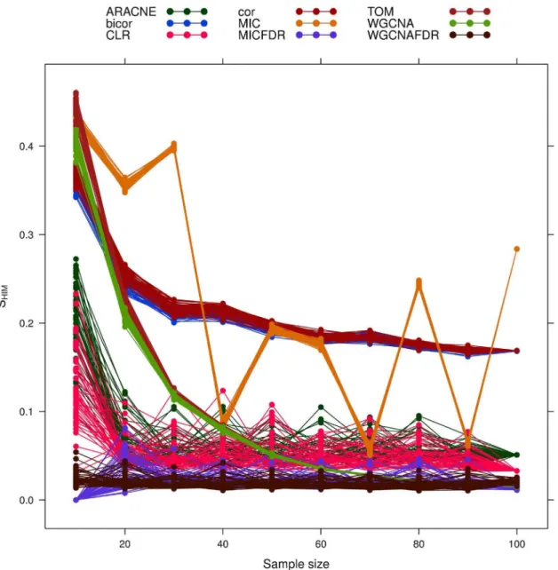
The definition of the Hamming distance is the following: Figure 8. Yeast-like simulated data: effect of increasing sample size on network reconstruction stabilitySHIM.Different network inference algorithms are compared.

Stability Indicators in Network Reconstruction

I

I 1

0

N 0

(8)

Hamming(_N1,N2)~

X

1ƒi jƒN

jA(1)_ij {A(2)_ij _j:

To guarantee independence from the network dimension (number of nodes), we normalize the above function by the factor

g~Hamming(EN,FN)~N(N{1):

H(N1,N2)~

1 N(N{1)

X

jA(1)ij {A

(2)

ij j: ð1Þ

When_N1andN2are unweighted networks,H(N1,N2)is just

the fraction of different matching links (over the total number

N(N{1) of possible links) between the two graphs. In all cases, H(N1,N2)[½0,1, where the lower bound0is attained only for

identical networksA(1)_~_A(2) _{and the upper bound}₁_{is reached}

whenever the two networks are complementary

A(1)zA(2)~ _N{ _N~

0 1 1

1 0 1

1 1 0

0

B B @

1

C C A .

Among spectral distances, we consider the Ipsen-Mikhailov distance IM which has been proven to be the most robust in a wide range of situations [37,38]. Originally introduced in [36] as a tool for network reconstruction from its Laplacian spectrum, the definition of the Ipsen-Mikhailov metric follows the dynamical interpretation of a N–nodes network as a N–atoms molecule connected by identical elastic strings, where the pattern of connections is defined by the adjacency matrix of the correspond-ing network. In particular the connections between nodes in the Figure 9. Yeast-like simulated data: effect of increasing sample size on network reconstruction internal stabilitySI

HIM.Different network inference algorithms are compared.

6

=

1

(9)

network correspond to the bonds between atoms in the dynamical system and the adjacency matrix is its topological description.

We summarize here the mathematical details of the IM definition [36]. The dynamical properties of the oscillatory system are described by the set ofN differential equations

€

x xiz

XN

j~1

Aij(xi{xj)~0 for i~0, ,N{1 , ð2Þ

wherexiare the coordinates of the physical molecules. Since the adjacency matrix Adepends on the node labeling, we consider instead the Laplacian matrixL, which for an undirected network is defined as the difference between the degree matrix D (the diagonal matrix with vertex degrees as entries) andA:L~D{A. L is positive semidefinite and singular [39–42], and its set of eigenvalues 0~l0ƒl1ƒ ƒlN{1, i.e. the spectra of the

associated graph, provide the natural vibrational frequencies vi for the system modeled in Eq. 2: li~v2i, with l0~v0~0. The

spectral densityrfor a graph can be written as the sum of Lorentz

distributions

r(v,c)~_KX

N{1

i~1 c

(v{vi)2_z_c2 ,

where c is the common width and K is the normalization constant defined as

K~ 1

cNP

{1

i~1

Ð?

0 ₍_v{vd_iv)2zc2

,

so that ð?

0

r(v,c)dv~1. The scale parameter cspecifies the

half-width at half-maximum, which is equal to half the inter-quartile range. From the above definitions, the spectral distancec

Figure 11. Construction of an FDR-corrected correlation network. doi:10.1371/journal.pone.0089815.g011

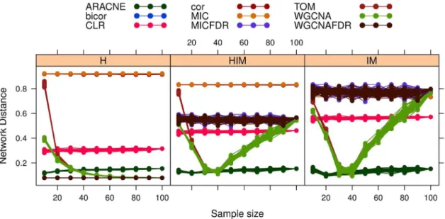
Figure 10. Yeast-like simulated data: effect of increasing sample size on network reconstruction accuracy measured as HIM distance and its components Hamming (H) and Ipsen-Mikhailov (IM) with respect to the gold standard.Different network inference algorithms are compared.

(10)

between two graphsGandHwith densitiesr_G(v,c)andr_H(v,c) can then be defined as

c(G,H)~

ffiffiffiffiffiffiffiffiffiffiffiffiffiffiffiffiffiffiffiffiffiffiffiffiffiffiffiffiffiffiffiffiffiffiffiffiffiffiffiffiffiffiffiffiffiffiffiffiffiffiffiffiffiffi ð?

0

r_G(v,c){r_H(v,c)

½ 2dv

s

:

The highest value of cis reached, for a given number of nodes

N, when evaluating the distance between N andFN. Definingc as the (unique [26]) solution of

c( N,FN)~1

we can now define the normalized Ipsen-Mikahilov distance IM as

IM(G,H)~_c(G,H)~

ffiffiffiffiffiffiffiffiffiffiffiffiffiffiffiffiffiffiffiffiffiffiffiffiffiffiffiffiffiffiffiffiffiffiffiffiffiffiffiffiffiffiffiffiffiffiffiffiffiffiffiffiffiffi ð?

0

r_G(v,c){r_H(v,c)

½ 2dv

s

,

so thatIM(G,H)[_½0,1with the upper bound attained only for (G,H)~(EN,FN).

Finally, the generalized HIM distance is defined by the one-parameter family of product metrics linearly combining with a factor j[_½0,z?) the normalized Hamming distance H and the normalized Ipsen-Mikhailov IM distance, further normalized by the factorpffiffiffiffiffiffiffiffiffiffi1zjto set its upper bound to 1:

HIMj(N1,N2)~

1 ffiffiffiffiffiffiffiffiffiffi 1zj p

ffiffiffiffiffiffiffiffiffiffiffiffiffiffiffiffiffiffiffiffiffiffiffiffiffiffiffiffiffiffiffiffiffiffiffiffiffiffiffiffiffiffiffiffiffiffiffiffiffiffiffiffiffiffiffi H(N1,N2)2zj:IM(N₁,N₂)2

q

:

Obviously,HIM0~H and lim

j?z?

HIMj~IM. For example,

the flexibility introduced byjcan be used to focus attention more on structure than on local editing changes whenHIMjis used to

generate a kernel function for classification tasks (e.g. on brain networks).

In what follows we will mostly deal with the casej~1, and omit the subscript j for brevity. The relative effect of the two components is exemplified in Fig. 1A-D. The three small size networks (5 nodes) NA,NB, andNC in Fig. 1A differ from each other in only two edges but NA and NC are isomorphic and diverse fromNB, as correctly picked up by the HIM distance (see table in Fig. 1C). Similarly, HIM, H and IM provide different values when four edges are cut from on the larger (50 nodes)G4

network, at different levels of the graph structure. Larger effects are caused by the elimination of the four red edges connecting the four submodules with differences up to 10 times larger for IM with respect to H (see table in Fig. 1D).

The HIM distance can be represented in the _½0,1|_½0,1 Hamming/Ipsen-Mikhailov space, where a point P(x,y) repre-sents the distance between two networks N1 and N2 whose

coordinates arex~H(N1,N2)andy~IM(N1,N2)and the norm

ofPispffiffiffiffiffiffiffiffiffiffi1zjtimes the HIM distanceHIM(N1,N2). The same

holds for weighted networks, provided that the weights range over

½0,1. In Fig. 2 we provide an example of this representation by evaluating the HIM distance between networks of four nodes, namely networks A, B, E (empty) and F (full) in the left panel of Fig. 2. If the Hamming/Ipsen-Mikhailov space is roughly split into four quadrants I, II, III, and IV, then two networks whose distance is mapped in quadrant I are close both in terms of matching links and of structure, while those falling in quadrant III differ with respect to both characteristics. Networks corresponding to a point in quadrant II have many common links, but different structures, while a point in quadrant IV indicates two networks with few common links, but with similar structure.

Full mathematical details about the HIM distance and its two components H and IM can be found in [26].

The Network Stability Indicators (NetSI)

The mathematical and operational definition of the four NetSI indicators are introduced in Fig. 3. The first two are the stability indicatorsSdand the internal stability indicatorSId, which concern

the stability of the whole reconstructed network. The former measures the distances between the network inferred on the whole dataset against the networks inferred from the resampled subsets. The latter measures all the mutual distances within the networks inferred from the resampled subsets. The other two indicators, the edge weight stability indicatorSw and the node degree stability indicatorSd, concern instead the stability of the single links and nodes, in terms of mutual variability of their respective weight and degree. In all cases, smaller indicator values correspond to more stable objects.

We adoptd~HIM, except for the first experiment where we show also the stability ford~Handd~IM. As the HIM distance is defined also on directed networks, the extension of the NetSI family to the directed case is straightforward. A graphical representation of the procedure is provided in Fig. 4. For all experiments reported in this paper, we usedn~s{1,r~1 (leave-one-out stability, LOO for short), and20different instances of k-fold cross validation (discarding the test portion) fork~2,4,10(k2, k4andk10), and thusn~s(k{1)

k andr~20k.

Stability of network inference algorithms

As a first application, we test the difference in stability of the reconstruction process for a set of alternative network co-expression inference algorithms.

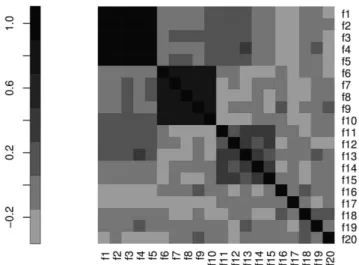
Figure 12. The correlation matrix MT used to generate the synthetic datasetT.

E

(11)

The most famous representative of the correlation-based approaches is surely the Weighted Gene Correlation Network Analysis (WGCNA) [30,43]. In this case the co-expression similarity is defined as a function of the absolute correlation. We adopt as similarity score: (i) the simple absolute Pearson correlation (labelled as ‘‘cor’’), (ii) a more sophisticated version with soft-thresholding,i.e., the similarity is defined as a power of the absolute correlation (we adopt the default value six as in the

WGCNAR package), or (iii) the biweight midcorrelation (‘‘bicor’’ for short) [30,44], which is more robust to outliers than the Pearson correlation, and (iv) the Maximal Information Coefficient (labeled as MIC). MIC is a recent association measure based on mutual information and belongs to the Maximal Information-based Nonparametric Exploration (MINE) statistics [44–48]. In all cases we obtain a weighted network with link strength ranging from 0 to 1.

The Topological Overlap Measure (TOM) replaces the original co-expression similarity with a measure of interconnectedness

(between pairs of nodes) based on shared neighbors [30,43]. TOM can be seen as a filter for cutting away weak connections, thus leading to more robust networks than WGCNA.

The Context Likelihood of Relatedness (CLR) approach [29] scores the interactions by using the mutual information between the corresponding gene expression levels, coupled with an adaptive background correction step. Although suboptimal if the number of nodes is much larger than the number of variables, it was observed that CLR performs well in terms of prediction accuracy and some CLR predictions in literature were recently validated experimen-tally [49].

The Algorithm for the Reconstruction of Accurate Cellular Networks (ARACNE) is another approach relying on mutual information, which was originally developed for inferring regula-tory networks of mammalian cells [28]. It starts with a graph where each pair of nodes are connected if their association is above a chosen threshold. In order to avoid the false positive problem, Figure 13. Synthetic datasetT: correlation networks inferred by using (A) WGCNA [W], (B) (absolute) Pearson with FDR correction atp-value10{4_[C(₁₀{4_{)] and (C) MIC [M].}_{Node label}_i_{corresponds to feature}_f

i, node size is proportional to node degree and link colors identify different classes of link weights.

(12)

that usually affects co-expression networks, we then apply the Data Processing Inequality (DPI) procedure for removing the weakest edge of each triplet, thus pruning the majority of undirected links. A unique interface to all the mentioned algorithms is integrated in the stability analysis tools in thenettoolspackage, based on their

Bioconductor and CRAN implementations: minet for ARACNE

and CLR,WGCNAfor WGCNA, TOM and bicor, andminervafor MIC.

Results and Discussion

Stability is modularity invariant

We demonstrate the invariance of the NetSI family with respect to network modularity in a controlled situation. We show that the proposed stability evaluation framework is not affected by various network structures for nine reconstruction algorithms. Moreover, we demonstrate that this property is maintained both if we adopt the HIM metric for theSdindicator computation and we use the

two components H and IM separately.

Data generation. We created a set of networksGm with 50 nodes each withm(wheremranges from 1 to 10) fully connected subgroups, which are linked to each other with a single edge. For m~₁we obtain a fully connected network (without loops), while the resulting networks formw1are displayed in Fig. 5. For each networkGmwe report its modularity value and density in Tab. 1. The simulated gene expression values corresponding to the networksGm are generated loading the corresponding adjacency matrices in the Gene Net Weaver (GNW) simulator [50]. Specifically, the tool is used to create of simulated transcription datasets after a random initialization of each network’s regulatory

dynamics through a pre-loaded kinetic model [23]. Moreover it is possible to generate a steady-state dataset or a set of time series, which describes the network response to a perturbation, followed by perturbation removal until the steady state is reached. Thus, we chose to generate in one shot 50 time-series (one for each sample) with default parameter settings and to consider only the initial time point, since t~0 corresponds to the wild-type steady state. Summarizing, we generated 10 synthetic datasets having a simulated expression level for 50 ‘‘genes’’ and 50 ‘‘samples’’.

Results. We inferred networks from the 10 datasets with nine algorithms: ARACNE, CLR, cor, TOM, bicor, WGCNA and MIC, where the last two were also used with a permutation-based FDR filter (for details, see Subsection ‘‘FDR control effect on correlation networks’’).

The stability analysis with three possible network metrics (HIM, H and IM) on networks inferred with the nine mentioned approaches is reported in Fig. 6. In all cases, the stabilitySdvaries

less than 0.06 across different modularity values, as detailed in Tab. 2. Hence, the stability indicator is not affected by different modular structures. However, reconstruction accuracy depends on modularity (or density), as shown by a comparison with the gold standard (Fig. 7), in which a lower distance from the gold standard is found for sparser networks for all methods.

Inference on synthetic yeast-like networks

We investigated the behavior of the NetSI stability indicators for different sample sizes on a yeast-like dataset, again simulated by GNW.

Data Description. We considered a subnetwork of the Yeast transcriptional regulatory network available in GNW, namely the

Table 3.Synthetic datasetT: stability (SHIMandSHIMI ) on networks inferred by MIC, WGCNA, and CORFDR(2).

A k S_HIM _{CI (min; max)} _{Range (min; max)} SI

HIM CI (min; max) Range (min; max)

MIC LOO 0.008 (0.007; 0.008) (0.004; 0.011) 0.008 (0.008; 0.008) (0.003; 0.014)

MIC k10 0.052 (0.051; 0.052) (0.041; 0.067) 0.021 (0.021; 0.021) (0.014; 0.036)

MIC k4 0.055 (0.054; 0.057) (0.040; 0.071) 0.031 (0.031; 0.031) (0.022; 0.045)

MIC k2 0.139 (0.134; 0.142) (0.112; 0.158) 0.047 (0.047; 0.048) (0.035; 0.067)

WGCNA LOO 0.005 (0.005; 0.006) (0.001; 0.015) 0.008 (0.008; 0.008) (0.002; 0.023) WGCNA k10 0.021 (0.020; 0.022) (0.011; 0.040) 0.028 (0.028; 0.028) (0.012; 0.064) WGCNA k4 0.039 (0.037; 0.041) (0.020; 0.062) 0.046 (0.046; 0.047) (0.025; 0.088) WGCNA k2 0.070 (0.065; 0.076) (0.037; 0.108) 0.070 (0.069; 0.071) (0.042; 0.117) CORFDR(10{2₎ _LOO _0.015 _{(0.013; 0.016)} _{(0.005; 0.035)} _0.017 _{(0.017; 0.017)} _{(0.001; 0.047)} CORFDR(10{2₎ _k₁₀ _0.023 _{(0.022; 0.025)} _{(0.007; 0.074)} _0.028 _{(0.027; 0.028)} _{(0.002; 0.102)} CORFDR(10{2₎ _k₄ _0.031 _{(0.028; 0.034)} _{(0.010; 0.069)} _0.034 _{(0.034; 0.035)} _{(0.006; 0.096)} CORFDR(10{2₎ _k₂ _0.045 _{(0.039; 0.054)} _{(0.014; 0.107)} _0.050 _{(0.048; 0.051)} _{(0.006; 0.152)} CORFDR(5:10{3) LOO 0.029 (0.028; 0.031) (0.003; 0.048) 0.018 (0.018; 0.018) (0.000; 0.054)

CORFDR(5:10{3) k10 0.025 (0.024; 0.027) (0.004; 0.054) 0.024 (0.024; 0.024) (0.001; 0.083)

CORFDR(5:₁₀{3) k4 0.025 (0.023; 0.028) (0.006; 0.056) 0.032 (0.032; 0.033) (0.004; 0.099)

CORFDR(5:10{3) k2 0.033 (0.028; 0.038) (0.008; 0.070) 0.044 (0.042; 0.045) (0.002; 0.121)

CORFDR(10{4₎ _LOO _0.010 _{(0.008; 0.013)} _{(0.000; 0.044)} _0.013 _{(0.013; 0.014)} _{(0.000; 0.045)} CORFDR(10{4₎ _k₁₀ _0.010 _{(0.009; 0.012)} _{(0.000; 0.053)} _0.014 _{(0.014; 0.015)} _{(0.000; 0.055)} CORFDR(10{4₎ _k₄ _0.009 _{(0.007; 0.012)} _{(0.001; 0.049)} _0.014 _{(0.014; 0.014)} _{(0.001; 0.054)} CORFDR(10{4₎ _k₂ _0.009 _{(0.007; 0.013)} _{(0.001; 0.031)} _0.014 _{(0.013; 0.015)} _{(0.001; 0.040)}

IndicatorsSHIMandSI

HIM, 95% Student bootstrap confidence intervals and range for different instances of the MIC, WGCNA and CORFDR(2) networks for different values of data subsampling.

(13)

InSilicoSize100-Yeast2 dataset with 100 nodes, originally a DREAM3 benchmark, generating 100 samples with default parameter configuration, including noise level, for wild-type steady state (the synthetic datasetY).

Results. We randomly extracted 10 subsets of different sample size N in _f10,20,30,40,50,60,70,80,90,100_g, replicating the subset extraction procedure 50 times for each N. For each combination ofN resampling, we inferred the network with the same nine algorithms used in the previous experiment.

As a general trend, stability decreases for larger sample size (see Fig. 8). TheSHIM stability curves for the two popular methods

ARACNE and CLR drop quickly after 20% of the sample size, improving over Pearson and bicor. TOM and WGCNA are more stable but require at least 50% of the data. The standard MIC-based method with the default parameter (a~0:6) is much

smoothed by the FDR correction. Overall, the FDR corrected methods are the most stable even for small samples. TOM and

WGCNA have the best internal stabilitySI

HIM(Fig. 9), followed by

the FDR-corrected methods.

Given that a gold standard is available for the simulated data in Y, we can compare the stability performance with reconstruction accuracy in terms of HIM and its components for the nine methods (Fig. 10). On this dataset, accuracy is independent of sample size, except for WGCNA and TOM which have an optimal range (N~f30,40g), given by their soft thresholding procedures. Note that the source Yeast subnetwork is unweighted while all methods return a weighted network: a10{3

threshold was thus applied to binarize the reconstructed network before computing the distances. Hence, MIC, cor and bicor perform badly as they lack an internal thresholding procedure; the FDR corrected methods have better but still mediocre results, slightly improved by CLR. On this dataset, WGCNA-FDR yields sparse networks (less than 20 edges) with small Hamming distances from the gold standard as they both have low density; however they have strongly different spectral structure from the gold standard, Figure 14. Synthetic dataset T: representation of SHIM and SIHIM stability indicators (with confidence intervals) for different instances of the FDR-corrected correlation networks, CORFDR(10{2_{), CORFDR(}₅_:₁₀{3_{), and CORFDR(}₁₀{4_{), WGCNA and MIC} networks on the datasetT and for different values of data subsampling.

(14)

as captured by the IM component. Finally, ARACNE achieves fair stability here as well as the highest accuracy.

The effect of FDR control on stability

We aim to assess differences in the stability of correlation networks inferred by an ad-hoc set of synthetic signals similar to expression data whenever inference is computed with or without False Discovery Rate (FDR) control.

FDR control for correlation networks. For an introduction to FDR methods, see for instance [51]. The procedure considered in this paper is explicitly described in Fig. 11. The FDR control defines a rule for choosing which edges to trust, and thus to keep,

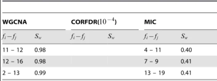
Table 4.Synthetic datasetT: top ranked links for edge weight stabilitySw on networks inferred by WGCNA, CORFDR(2~₁₀{4), and MIC.

WGCNA CORFDR( ) MIC

fi{fj Sw fi{fj Sw fi{fj Sw

1 – 3 0.03 1 – 3 0.03 3 – 4 0.20

2 – 3 0.04 3 – 4 0.04 2 – 3 0.20

1 – 2 0.04 2 – 3 0.04 1 – 3 0.21

1 – 4 0.04 1 – 4 0.05 3 – 5 0.22

3 – 4 0.04 3 – 5 0.05 1 – 2 0.23

2 – 4 0.04 1 – 2 0.05 1 – 5 0.25

4 – 5 0.04 2 – 4 0.05 1 – 4 0.26

2 – 5 0.05 2 – 5 0.06 4 – 5 0.27

1 – 5 0.05 4 – 5 0.06 7 – 10 0.28

3 – 5 0.05 1 – 5 0.06 7 – 8 0.29

6 – 8 0.08 6 – 8 0.08 6 – 8 0.29

8 – 10 0.10 7 – 8 0.09 6 – 10 0.30

7 – 8 0.11 8 – 10 0.10 1 – 20 0.31

7 – 9 0.11 8 – 9 0.11 2 – 4 0.31

8 – 9 0.11 6 – 7 0.11 8 – 10 0.31

9 – 10 0.11 7 – 10 0.12 2 – 5 0.32

6 – 7 0.11 7 – 9 0.12 9 – 10 0.32

7 – 10 0.12 9 – 10 0.13 7 – 20 0.33

6 – 10 0.13 6 – 9 0.13 14 – 16 0.33

6 – 9 0.14 6 – 10 0.15 5 – 17 0.35

11 – 13 0.33 6 – 7 0.35

14 – 15 0.41 11 – 17 0.36

13 – 14 0.46 6 – 9 0.36

12 – 13 0.58 1 – 10 0.37

12 – 15 0.60 10 – 11 0.37

11 – 14 0.62 10 – 20 0.37

13 – 15 0.71 4 – 17 0.37

11 – 15 0.78 2 – 8 0.37

14 – 18 0.78 4 – 10 0.37

3 – 11 0.83 6 – 13 0.37

5 – 11 0.83 2 – 14 0.37

1 – 11 0.84 9 – 11 0.38

4 – 11 0.85 15 – 16 0.38

3 – 10 0.87 15 – 17 0.38

5 – 16 0.89 7 – 13 0.39

8 – 17 0.89 9 – 18 0.39

2 – 11 0.91 12 – 19 0.39

8 – 12 0.91 6 – 18 0.39

4 – 13 0.91 8 – 9 0.39

1 – 13 0.93 4 – 18 0.39

3 – 13 0.93 16 – 17 0.39

8 – 13 0.94 4 – 19 0.39

9 – 17 0.94 16 – 19 0.39

1 – 16 0.95 7 – 19 0.40

1 – 10 0.95 5 – 8 0.40

14 – 16 0.97 14 – 15 0.40

5 – 10 0.97 13 – 15 0.40

Table 4.Cont.

WGCNA CORFDR( ) MIC

fi{fj Sw fi{fj Sw fi{fj Sw

11 – 12 0.98 4 – 11 0.40

12 – 16 0.98 7 – 9 0.41

2 – 13 0.99 13 – 19 0.41

The links are ordered bySwacross all 20 resamplings ofk10cross validation, for the three algorithms; the table includes the top 50 links for WGCNA and MIC, and all 20 links found by CORFDR(2~10{4_).

Table 5.Synthetic datasetT: nodes ranked by stability degreeSd on networks inferred by WGCNA,

CORFDR(2~10{4_{), and MIC.}

WGCNA CORFDR( ) MIC

fi Sd fi Sd fi Sd

4 0.17 16 0* 3 0.08

10 0.18 17 0* 19 0.08

3 0.20 18 0* 1 0.08

1 0.21 19 0* 4 0.09

9 0.23 20 0* 8 0.09

2 0.23 3 0.03 10 0.09

5 0.24 1 0.04 5 0.10

7 0.24 2 0.04 2 0.10

6 0.24 5 0.05 17 0.10

8 0.25 7 0.07 20 0.10

11 0.40 8 0.07 15 0.11

13 0.40 6 0.09 9 0.11

15 0.43 9 0.09 13 0.11

12 0.45 10 0.09 11 0.11

14 0.48 4 0.13 16 0.11

18 0.55 15 4.42 12 0.11

16 0.60 14 7.05 7 0.11

17 0.68 12 22.82 6 0.12

20 0.70 13 26.05 14 0.13

19 1.15 11 41.83 18 0.13

The 20 nodes are ordered bySdacross all 20 resamplings byk10cross validation. (*) indicates that range and mean are both zero.

10{4

(15)

during the network reconstruction phase. An edge weight is given by the correlation coefficient between the signal values of two nodesh,k:ahk~C(h,k)~jcor(xh,xk)j, wherecoris a correlation function. Ifmis the sample size, we wish to estimate the chance that a random permutation of the expression values may give a correlation value higher than C(h,k), thus removing the edge when this chance is larger than a permutational p-value2~10{z

, where z is a chosen level of significance (typically z~3). In practice, this test is implemented by counting how many times C(h,k) is smaller than the correlation betweens(xh)and t(xk), wheresandtare distinct permutations ofmobjects. We consider here the absolute Pearson correlation at different 2 levels

CORFDR(2), when compared with WGCNA [30,43] with default thresholding parameter, as well as with the Maximal Information Coefficient (MIC), a non-linear correlation measure defined within the Maximal Information-based Nonparametric Exploration (MINE) statistics [45–47]. Note that the FDR correction procedure can be implemented with different correla-tion measures, such as WGCNA-FDR and MIC-FDR considered in the previous section.

Data generation. In this example, the correlation networks are inferred from a dataset T of 100 samples of 20 features

ff1,. . .,f20g, via the Choleski decomposition (using the chol R

Figure 15. HCC-B dataset: CLR networks in the hairball representation inferred from the 4 subsets (A) Male Tumoral (MT), (B) Male non Tumoral (MnT), (C) Female Tumoral (FT), and (D) Female non Tumoral (FnT).Links are thresholded at weight 0.1, node position is fixed across the four networks, node dimension is proportional to the degree and edge width is proportional to link weight.

(16)

Figure 16. HCC-B dataset: CLR networks in the hiveplot representation inferred from the 4 subsets (A) Male Tumoral (MT), (B) Male non Tumoral (MnT), (C) Female Tumoral (FT), and (D) Female non Tumoral (FnT).Each plot consists of six axes with lines connecting points lying on the axes themselves. The axisa1pointing upwards collects all the nodes with (unweighted) degree 0 or 1;a2, the next axis moving clockwise, is a copy ofa1; the following two axes include all nodes with degree 2, while on the remaining two axes lie all nodes with degree 3 or more. Different colors indicate different degree. Nodes on axes are ranked by degree. Lines between two consecutive axes show the network’s edges and edge color is inherited by the node with smaller degree. Note the absence of links between nodes of degreee 1 and 2 in the FT case, and the smaller amount of connections between higher degree nodes in the MnT case with respect to the other three cases.

Figure 17. HCC-B dataset: mutual HIM distances for CLR inferred networks.Comparison of the four networks Male Tumoral (MT), Male non Tumoral (MnT), Female Tumoral (FT) and Female non Tumoral (FnT) reconstructed from the whole corresponding subsets in Tab. (A) and in the derived 2D multidimensional scaling plot (B).

(17)

function) of its correlation matrix MT, randomly generated according to the following three constraints:

cor(fi,fj)&

0:9 for 1ƒijƒ5

0:7 for 6ƒijƒ10

0:4 for 11ƒijƒ15 ,

0

B @

wherecor is the Pearson correlation. The correlation matrix MT is plotted in Fig. 12: the correlation values in the three groups defined by the above constraints represent true relations between the variables, while all other smaller correlation values are due to the underlying random generation model forMT.

Results. Starting from the datasetT, we built five correlation

networks, using MIC, WGCNA, and CORFDR(2) withp-values

2~10{2_,5

:10{3,10{4.

The three networks displayed in Fig. 13(A-C) were inferred with

WGCNA, CORFDR(10{4_{) and MIC respectively. WGCNA and}

MIC generate two fully connected networks with a majority of

weak links, while CORFDR correctly selects only links within the two disjoint sets of nodes _ffi:1ƒiƒ5g and ffi:6ƒiƒ10g, corresponding to the strongest correlations in the matrixMT.

Note that although both WGCNA and CORFDR(10{4₎

employ corinternally, the two algorithms can lead to different results. Indeed the soft thresholding procedure in WGCNA [43] defines weights as aij~jcor(xi,xj)jb for b~6, while for CORFDR(10{4_{) is}_a

ij~jcor(xi,xj)jif jFT4(i,j)jƒ1, according to the definition in Fig. 11.

Stability estimates are also less variable with the FDR corrected methods. We comparedk-fold cross-validation estimates ofSHIM

and SIHIM for the five networks, with k~1,2,4,10. Results are

presented in Tab. 3 and displayed in Fig. 14. On this dataset, SHIM ranges over ½0:001,0:108for WGCNA, ½0:004,0:158for

MIC, and only over½0:000,0:053for CORFDR(10

{4_{). Note that}

estimates are both smaller and less variable for the smallest p-value, as noise effects are filtered. Hence, the use of a FDR control procedure helps stabilize the correlation based inference proce-dure, improving the performance of WGCNA, already one of the more robust options for real data [52].

Table 6.HCC-B dataset:SHIMandSIHIMstatistics for FnT network.

Algorithm k S_HIM

S_HIM_CI (min; max)

S_HIM_Range

(min; max) SI

HIM

SI

HIMCI

(min; max)

SI HIMRange (min; max)

ARACNE LOO 0.007 (0.006; 0.009) (0.002; 0.018) 0.008 (0.008; 0.009) (0.001; 0.045)

ARACNE k2 0.037 (0.030; 0.045) (0.007; 0.097) 0.032 (0.031; 0.033) (0.002; 0.179)

ARACNE k4 0.024 (0.021; 0.027) (0.004; 0.060) 0.022 (0.022; 0.023) (0.002; 0.134)

ARACNE k10 0.013 (0.012; 0.014) (0.003; 0.036) 0.014 (0.013; 0.014) (0.000; 0.081)

CLR LOO 0.022 (0.017; 0.027) (0.003; 0.048) 0.030 (0.028; 0.032) (0.001; 0.094)

CLR k2 0.094 (0.071; 0.117) (0.006; 0.257) 0.119 (0.113; 0.124) (0.006; 0.391)

CLR k4 0.062 (0.054; 0.072) (0.005; 0.203) 0.080 (0.078; 0.082) (0.003; 0.307)

CLR k10 0.032 (0.029; 0.035) (0.002; 0.093) 0.045 (0.044; 0.045) (0.000; 0.179)

cor LOO 0.021 (0.017; 0.026) (0.006; 0.051) 0.031 (0.030; 0.032) (0.002; 0.122)

cor k2 0.117 (0.104; 0.133) (0.059; 0.221) 0.145 (0.143; 0.147) (0.016; 0.431)

cor k4 0.070 (0.065; 0.078) (0.023; 0.172) 0.093 (0.092; 0.094) (0.008; 0.347)

cor k10 0.038 (0.036; 0.041) (0.014; 0.120) 0.053 (0.053; 0.054) (0.000; 0.279)

bicor LOO 0.026 (0.022; 0.031) (0.012; 0.057) 0.036 (0.035; 0.037) (0.004; 0.136)

bicor k2 0.117 (0.105; 0.132) (0.072; 0.227) 0.151 (0.148; 0.153) (0.015; 0.445)

bicor k4 0.076 (0.070; 0.083) (0.033; 0.180) 0.100 (0.099; 0.101) (0.007; 0.367)

bicor k10 0.044 (0.041; 0.047) (0.019; 0.126) 0.060 (0.059; 0.060) (0.000; 0.286)

WGCNA LOO 0.015 (0.013; 0.018) (0.005; 0.033) 0.019 (0.019; 0.020) (0.003; 0.078)

WGCNA k2 0.099 (0.086; 0.114) (0.035; 0.198) 0.094 (0.092; 0.096) (0.017; 0.341)

WGCNA k4 0.048 (0.043; 0.055) (0.015; 0.115) 0.057 (0.056; 0.057) (0.007; 0.251)

WGCNA k10 0.026 (0.025; 0.028) (0.006; 0.081) 0.033 (0.033; 0.034) (0.000; 0.187)

MINE LOO 0.035 (0.031; 0.039) (0.018; 0.054) 0.040 (0.040; 0.041) (0.003; 0.096)

MINE k2 0.138 (0.125; 0.157) (0.084; 0.277) 0.149 (0.146; 0.151) (0.020; 0.482)

MINE k4 0.150 (0.138; 0.161) (0.050; 0.259) 0.105 (0.105; 0.106) (0.007; 0.335)

MINE k10 0.067 (0.064; 0.071) (0.029; 0.138) 0.067 (0.066; 0.067) (0.000; 0.253)

TOM LOO 0.020 (0.017; 0.025) (0.007; 0.047) 0.025 (0.024; 0.026) (0.003; 0.108)

TOM k2 0.133 (0.115; 0.154) (0.046; 0.271) 0.117 (0.114; 0.119) (0.011; 0.467)

TOM k4 0.065 (0.057; 0.075) (0.017; 0.161) 0.073 (0.072; 0.074) (0.010; 0.348)

TOM k10 0.035 (0.033; 0.038) (0.007; 0.116) 0.043 (0.043; 0.044) (0.000; 0.268)

Values of the indicatorsSHIMandSI

HIMtogether with bootstrap confidence intervals and range for the inferred networks for different values of data subsampling. doi:10.1371/journal.pone.0089815.t006

(18)

Results for weight stability and degree stability are listed in Tab. 4 and Tab. 5, respectively, comparing the rankings for WGCNA, CORFDR(10{4_{) and MIC for a} _k₁₀ _{resampling. The stability}

indicators give information consistent with the structure of the starting correlation matrixMT: inference by WGCNA (Fig. 13 A) exactly reconstructs the block structure with three subnetworks (blue:Corr^0

:9, greenCorr^0:7, orange:Corr^0:4), while the

FDR corrected version (Fig. 13 B) selects only two subnetworks corresponding to the two top correlated feature blocks of Fig. 12. In the WGCNA case, the top 20 most stable links (Tab. 4) are those of the two cliques F1,5~ffi:1ƒiƒ5g and F6,10~ffi:6ƒiƒ10g with largest correlation values in MT. The correct block structure is found by CORFDR(10{4

) with

approximately the same values of Sw found by the WGCNA

network, where minor differences are due to the different thresholding procedures.

The F11,15~ffi:11ƒiƒ15g variables (mutual correlation of about 0.3 imposed by design ofMT) are also mostly top ranked links for WGCNA, but with larger instability values (0.33–0.78 vs. 0.03–0.14). The remaining links are the least stable, withSwvalues always larger than 0.83: they are the randomly correlated links of

MT. Similar but not identical results are found for the networkM, as expected given that the MIC statistic aims at detecting generic associations between variables and it is expected to have reduced statistical power with low sample sizes. The structure of the network (Fig. 13 C) does not reflect the design linear correlation structure. Indeed, several links are ranked differently as the expected: although many links in theF1,5 and F6,10 groups are

highly ranked, some of them can also be found in much lower positions (e.g. 6–7, 6–9, or 7–9 are ranked lower than 20; 7–10, 7–8 are ranked higher than 2–4, 2–5; 1–20, 7–20, 14–16, and 5–17 are ranked within the top 20 links).

Similar considerations hold for the ranking of the most stable nodes: for WGCNA, the top-ranked nodes are theF1,5 and the

F6,10(with similarSdvalues); those inF11,15come next, leaving the

remaining five as the least stable with higher Sd values. These nodes are trivially the most stable for CORFDR(10{4_{) as they are}

never wired to any other node in any of the resampling and thus theirSd values are void.

The nodes F1,5|F6,10 then follow in the ranking with small

associated values, and the nodes F11,15 close the standing with

definitely higher values. In fact, although the nodesF11,15 have

Table 7.HCC-B dataset:SHIMandSIHIMstatistics for FT network.

Algorithm k S_HIM

S_HIMCI (min; max)

S_HIMRange

(min; max) S_HIMI

S_HIMI CI (min; max)

S_HIMI Range (min; max)

ARACNE LOO 0.007 (0.006; 0.010) (0.001; 0.024) 0.009 (0.009; 0.010) (0.001; 0.053) ARACNE k2 0.032 (0.024; 0.053) (0.008; 0.221) 0.036 (0.034; 0.039) (0.003; 0.405) ARACNE k4 0.016 (0.014; 0.018) (0.005; 0.054) 0.019 (0.019; 0.020) (0.002; 0.137) ARACNE k10 0.012 (0.010; 0.013) (0.002; 0.061) 0.014 (0.014; 0.014) (0.000; 0.120)

CLR LOO 0.022 (0.016; 0.032) (0.002; 0.093) 0.032 (0.030; 0.035) (0.001; 0.143)

CLR k2 0.069 (0.056; 0.082) (0.006; 0.154) 0.089 (0.084; 0.093) (0.005; 0.250)

CLR k4 0.057 (0.049; 0.066) (0.004; 0.190) 0.078 (0.076; 0.080) (0.003; 0.305)

CLR k10 0.040 (0.037; 0.044) (0.002; 0.177) 0.054 (0.054; 0.055) (0.000; 0.143)

cor LOO 0.019 (0.016; 0.024) (0.008; 0.044) 0.028 (0.028; 0.029) (0.003; 0.105)

cor k2 0.122 (0.111; 0.138) (0.079; 0.221) 0.144 (0.142; 0.147) (0.014; 0.346)

cor k4 0.067 (0.063; 0.073) (0.036; 0.141) 0.088 (0.087; 0.088) (0.007; 0.274)

cor k10 0.037 (0.036; 0.039) (0.019; 0.083) 0.051 (0.051; 0.051) (0.000; 0.196)

bicor LOO 0.022 (0.019; 0.027) (0.012; 0.049) 0.031 (0.031; 0.032) (0.004; 0.108)

bicor k2 0.116 (0.107; 0.130) (0.073; 0.217) 0.148 (0.146; 0.150) (0.012; 0.364)

bicor k4 0.069 (0.065; 0.074) (0.038; 0.137) 0.092 (0.091; 0.092) (0.009; 0.282)

bicor k10 0.040 (0.039; 0.042) (0.022; 0.085) 0.055 (0.055; 0.055) (0.000; 0.202) WGCNA LOO 0.010 (0.008; 0.013) (0.003; 0.025) 0.013 (0.013; 0.014) (0.002; 0.070)

WGCNA k2 0.109 (0.095; 0.124) (0.026; 0.194) 0.070 (0.068; 0.072) (0.016; 0.269)

WGCNA k4 0.043 (0.039; 0.049) (0.008; 0.099) 0.039 (0.038; 0.039) (0.007; 0.182)

WGCNA k10 0.022 (0.020; 0.023) (0.005; 0.066) 0.024 (0.024; 0.024) (0.000; 0.141)

MINE LOO 0.031 (0.028; 0.034) (0.016; 0.051) 0.032 (0.031; 0.032) (0.003; 0.095)

MINE k2 0.138 (0.128; 0.149) (0.094; 0.216) 0.129 (0.128; 0.131) (0.007; 0.321)

MINE k4 0.201 (0.194; 0.207) (0.132; 0.257) 0.088 (0.088; 0.089) (0.005; 0.243)

MINE k10 0.077 (0.075; 0.080) (0.040; 0.138) 0.054 (0.054; 0.054) (0.000; 0.193)

TOM LOO 0.015 (0.011; 0.019) (0.004; 0.038) 0.018 (0.017; 0.019) (0.002; 0.105)

TOM k2 0.148 (0.128; 0.170) (0.023; 0.269) 0.092 (0.090; 0.095) (0.012; 0.386)

TOM k4 0.060 (0.053; 0.069) (0.011; 0.143) 0.053 (0.052; 0.054) (0.006; 0.272)

TOM k10 0.031 (0.029; 0.033) (0.006; 0.097) 0.033 (0.033; 0.033) (0.000; 0.212)

(19)

degree zero in the network CORFDR(10{4

) inferred from the whole T, some links connecting them have weight over the threshold in several resamplings. Note that the ranking values for MIC span a narrow range, with most of the nodes inF1,5in top

positions, in general yielding a weak relation with the structure of MT.

The weight and degree stability analysis for the other subsampling cases (LOO, k2and k10) are almost identical and thus not shown here.

miRNA networks for hepatocellular carcinoma

Investigating the relationships connecting human microRNA (miRNA) and how they evolve in cancer is a key issue for researchers in biology [53,54]. Hepatocellular carcinoma (HCC) is a notable example [55,56]: we test the NetSI indicators on a miRNA microarray hepatocellular carcinoma dataset with two phenotypes as a tool for differential network analysis. As CLR was used in the original paper, we applied this inference method and compared its stability with the reconstruction algorithms previ-ously employed on the synthetic datasets.

Data description. The HCC dataset (HCC-B) [31,32] is publicly available at the Gene Expression Omnibus (GEO) http:// www.ncbi.nlm.nih.gov/geo with accession number GSE6857. The dataset collects 482 tissue samples from 241 patients affected by HCC. For each patient, a sample from cancerous hepatic tissue and a sample from surrounding non-cancerous hepatic tissue are available, hybridized on the Ohio State University CCC MicroRNA Microarray Version 2.0 platform consisting of 11,520 probes measuring the expression of 250 non-redundant human and 200 mouse miRNAs. After imputation of missing values [57], probes corresponding to non-human (mouse and controls) miRNAs were discarded; samples for one patient (AN) were eliminated. We thus obtained a dataset of 240+240 paired samples described by 210 human miRNAs (210 males, 30 females). Thus HCC-B can be split into four subsets by combining the gender and disease status phenotypes, respectively for tissues of male cancer patients (MT), female cancer patients (FT) and the corresponding non cancer tissues (MnT and FnT).

For validation, we considered a second dataset (HCC-W) recently used to derive a signature of 30 miRNAs for hepatocel-lular carcinoma [58]. miRNA expression data for 166 subjects

Table 8.HCC-B dataset:SHIMandSIHIMstatistics for MnT network.

Algorithm k S_HIM

S_HIMCI (min; max)

S_HIMRange

(min; max) S_HIMI

ARACNE LOO 0.002 (0.002; 0.002) (0.001; 0.004) 0.002 (0.002; 0.002) (0.000; 0.011)

ARACNE k2 0.014 (0.011; 0.016) (0.003; 0.033) 0.012 (0.012; 0.012) (0.002; 0.056)

ARACNE k4 0.007 (0.006; 0.008) (0.003; 0.022) 0.008 (0.007; 0.008) (0.001; 0.046)

ARACNE k10 0.005 (0.004; 0.005) (0.002; 0.011) 0.005 (0.005; 0.005) (0.001; 0.027)

CLR LOO 0.002 (0.002; 0.002) (0.000; 0.009) 0.003 (0.003; 0.003) (0.000; 0.016)

CLR k2 0.033 (0.026; 0.041) (0.003; 0.104) 0.037 (0.035; 0.039) (0.002; 0.158)

CLR k4 0.018 (0.015; 0.022) (0.001; 0.067) 0.025 (0.024; 0.026) (0.001; 0.102)

CLR k10 0.009 (0.008; 0.010) (0.001; 0.034) 0.013 (0.013; 0.013) (0.001; 0.061)

cor LOO 0.003 (0.003; 0.004) (0.001; 0.020) 0.005 (0.005; 0.005) (0.000; 0.047)

cor k2 0.050 (0.044; 0.057) (0.028; 0.094) 0.065 (0.064; 0.066) (0.007; 0.219)

cor k4 0.031 (0.028; 0.034) (0.013; 0.080) 0.042 (0.041; 0.042) (0.005; 0.180)

cor k10 0.018 (0.017; 0.019) (0.007; 0.056) 0.025 (0.025; 0.025) (0.002; 0.134)

bicor LOO 0.004 (0.004; 0.004) (0.001; 0.011) 0.005 (0.005; 0.005) (0.000; 0.027)

bicor k2 0.046 (0.041; 0.054) (0.026; 0.103) 0.063 (0.062; 0.064) (0.009; 0.240)

bicor k4 0.031 (0.028; 0.034) (0.014; 0.093) 0.042 (0.042; 0.043) (0.005; 0.197)

bicor k10 0.018 (0.017; 0.019) (0.008; 0.050) 0.025 (0.024; 0.025) (0.002; 0.122)

WGCNA LOO 0.002 (0.002; 0.003) (0.000; 0.019) 0.003 (0.003; 0.003) (0.000; 0.039)

WGCNA k2 0.037 (0.032; 0.044) (0.009; 0.078) 0.044 (0.043; 0.045) (0.011; 0.181)

WGCNA k4 0.021 (0.019; 0.024) (0.006; 0.059) 0.026 (0.026; 0.027) (0.005; 0.132)

WGCNA k10 0.013 (0.012; 0.014) (0.003; 0.044) 0.016 (0.016; 0.016) (0.002; 0.100)

MINE LOO 0.005 (0.005; 0.005) (0.002; 0.008) 0.006 (0.006; 0.006) (0.000; 0.019)

MINE k2 0.132 (0.123; 0.143) (0.059; 0.199) 0.064 (0.063; 0.065) (0.006; 0.233)

MINE k4 0.052 (0.048; 0.058) (0.021; 0.126) 0.041 (0.040; 0.041) (0.004; 0.186)

MINE k10 0.019 (0.019; 0.021) (0.012; 0.055) 0.025 (0.025; 0.025) (0.002; 0.121)

TOM LOO 0.003 (0.003; 0.004) (0.000; 0.023) 0.004 (0.004; 0.004) (0.000; 0.052)

TOM k2 0.051 (0.043; 0.060) (0.011; 0.111) 0.058 (0.056; 0.059) (0.010; 0.253)

TOM k4 0.029 (0.026; 0.033) (0.007; 0.085) 0.035 (0.034; 0.035) (0.005; 0.193)

TOM k10 0.017 (0.016; 0.018) (0.003; 0.060) 0.021 (0.021; 0.021) (0.003; 0.138)

HIMtogether with bootstrap confidence intervals and range for the inferred networks for different values of data subsampling. doi:10.1371/journal.pone.0089815.t008

(20)

(paired samples for 141 males and 25 females), acquired with the CapitalBio custom two-channel microarray platform (692 probes), are available at GEO accession number GSE31384. Data are processed as normalized differential miRNA expression levels between tumors and non cancerous liver tissue data [58].

Results. Using the CLR algorithm we first generated the four networks inferred from the whole set of datasets and correspond-ing to the combinations of the two binary phenotypes, discardcorrespond-ing links with weight smaller than 0.1. Two different representations of the resulting graphs are shown in Fig. 15 and Fig. 16, respectively in hairball and hiveplot layouts [59]. The second visualization technique is particularly useful in highlighting differences between networks by disaggregating the network structure according to their node degree. The four networks have different structures: more high degree links are present for tumoral tissues (graphs for MT and FT: Fig. 16 A and C) than for controls (MnT, FnT). Their density values, defined as the ratio between the number of existing edges and the maximal number of edges for the given graph), are 0.0153 (MT), 0.0092 (MnT), 0.0206 (FT) and 0.0121 (FnT). The mutual HIM distances for the four networks are reported in Fig. 17 A, together with the corresponding

two-dimensional scaling plot (Fig. 17 B). The networks corre-sponding to the female patients (and, in particular, the FT inferred from cancer tissue) are different from those inferred for the male patients.

In order to explore network reconstruction reliability, we then computed the NetSI indicators and compared the results for CLR with other six reconstruction algorithms ARACNE, cor, TOM, bicor, WGCNA and MIC. The corresponding statistics for the four subsets and different subsampling (LOO,k2,k4, andk10) are listed in Tables 6–9 and summarized in Fig. 18. Both the resampling strategy and phenotypes have an impact on the network stability, differently for the seven methods: the networks corresponding to male patients have smaller values forSHIMand

SIHIM(and thus they are much more stable) than the

correspond-ing female counterparts. The leave-one-out stability for FT and FnT is worse than for k10 and k4 stability on MT and MnT. However phenotypes have a stronger effect than the resampling strategy. Note that while control and cancer networks display similar stability for males at all levels of subsampling ratio, the FT network is more stable than the matching FnT control networks;

Table 9.HCC-B dataset:S_HIM_andS_HIMI _{statistics for MT network.}

Algorithm k S_HIM

S_HIMCI (min; max)

S_HIMRange

(min; max) S_HIMI

ARACNE LOO 0.001 (0.001; 0.002) (0.000; 0.008) 0.002 (0.002; 0.002) (0.000; 0.017)

ARACNE k2 0.017 (0.014; 0.020) (0.004; 0.039) 0.012 (0.012; 0.013) (0.002; 0.054)

ARACNE k4 0.009 (0.008; 0.010) (0.002; 0.021) 0.008 (0.008; 0.008) (0.001; 0.039)

ARACNE k10 0.005 (0.005; 0.006) (0.001; 0.015) 0.005 (0.005; 0.005) (0.001; 0.033)

CLR LOO 0.002 (0.002; 0.002) (0.000; 0.018) 0.003 (0.003; 0.003) (0.000; 0.030)

CLR k2 0.040 (0.033; 0.051) (0.003; 0.146) 0.051 (0.048; 0.054) (0.003; 0.218)

CLR k4 0.024 (0.020; 0.029) (0.002; 0.099) 0.033 (0.032; 0.033) (0.001; 0.148)

CLR k10 0.011 (0.010; 0.013) (0.001; 0.048) 0.016 (0.016; 0.016) (0.001; 0.092)

cor LOO 0.003 (0.003; 0.004) (0.001; 0.013) 0.005 (0.005; 0.005) (0.000; 0.028)

cor k2 0.046 (0.041; 0.054) (0.029; 0.105) 0.063 (0.062; 0.064) (0.008; 0.254)

cor k4 0.028 (0.026; 0.030) (0.016; 0.052) 0.038 (0.037; 0.038) (0.005; 0.132)

cor k10 0.017 (0.016; 0.018) (0.008; 0.041) 0.023 (0.023; 0.023) (0.002; 0.101)

bicor LOO 0.004 (0.003; 0.004) (0.001; 0.013) 0.005 (0.005; 0.005) (0.000; 0.028)

bicor k2 0.049 (0.044; 0.058) (0.027; 0.112) 0.067 (0.066; 0.068) (0.009; 0.272)

bicor k4 0.029 (0.027; 0.031) (0.016; 0.061) 0.039 (0.039; 0.040) (0.004; 0.148)

bicor k10 0.018 (0.017; 0.019) (0.009; 0.042) 0.025 (0.025; 0.025) (0.002; 0.105)

WGCNA LOO 0.002 (0.002; 0.002) (0.000; 0.009) 0.003 (0.003; 0.003) (0.000; 0.020)

WGCNA k2 0.034 (0.029; 0.040) (0.009; 0.075) 0.038 (0.037; 0.039) (0.008; 0.175)

WGCNA k4 0.018 (0.016; 0.021) (0.006; 0.046) 0.022 (0.022; 0.023) (0.004; 0.122)

WGCNA k10 0.011 (0.010; 0.012) (0.002; 0.028) 0.013 (0.013; 0.013) (0.002; 0.075)

MINE LOO 0.006 (0.006; 0.006) (0.002; 0.010) 0.006 (0.006; 0.006) (0.000; 0.018)

MINE k2 0.173 (0.163; 0.183) (0.111; 0.242) 0.060 (0.059; 0.061) (0.004; 0.220)

MINE k4 0.065 (0.061; 0.070) (0.027; 0.117) 0.037 (0.036; 0.037) (0.003; 0.149)

MINE k10 0.020 (0.019; 0.021) (0.011; 0.046) 0.024 (0.024; 0.024) (0.001; 0.099)

TOM LOO 0.003 (0.003; 0.003) (0.000; 0.012) 0.003 (0.003; 0.004) (0.000; 0.028)

TOM k2 0.046 (0.039; 0.054) (0.011; 0.102) 0.049 (0.047; 0.051) (0.008; 0.246)

TOM k4 0.025 (0.022; 0.028) (0.007; 0.062) 0.029 (0.029; 0.030) (0.003; 0.168)

TOM k10 0.015 (0.013; 0.016) (0.003; 0.038) 0.017 (0.017; 0.017) (0.002; 0.102)

Values of the indicatorsS_HIM_and_SI

(21)

this is evident when the size of the subset used for inference gets smaller, in particular fork2.

To validate the interest of the stability analysis in terms of biological relevance and reproducibility, we applied theSwweight stability indicator and ranked accordingly the links for networks inferred with CLR on the MT, MnT, FT, FnT subsets. Our hypothesis is that, in practical cases, stability may be either an effect of real biological relevance of the link or highlight trivial relationships between nodes. In the former situation, we expect that stable links have a better chance of being reproduced on new datasets. However, the comparison between miRNA studies is often haunted by the significant changes across releases of the annotation datasets. It is not uncommon that a miRNA may get discarded or unified with others in a newer release, or that miRNA symbols may just be remapped to different sequences.

As an experiment, we considered the first six top ranked edges for the four networks, obtaining seven distinct pairs of miRNAs according to the original annotation (Tab. 10). As reported by the original GEO platform (accession number GPL4700), the HCC-B dataset [31] used the miRBase June 2004 or information collected from literature. The two miRNA 321No1 and hsa-mir-321No2 had the same mature Sanger registry name in the miRBase June 2004, and were eliminated and marked as tRNA in the June 2013 version. Not surprisingly they define a link (link (a) in the table) which is trivially the most stable for all four networks, regardless of the phenotypes. Similarly the pairs of miRNA defining the links (b) and (c) can be found to align to the same sequences by considering miRBase June 2013. Note that (c) is

associated with the mature miR21, which is a known oncomir [60]. The hsa-mir-219-1 in link (d) is one of the 20 miRNAs in the signature proposed by Budhu and colleagues [31]; in our table it is differently stable for gender, which is consistent with being associated with estrogen regulation and overexpressed in breast cancer [61,62]. The link (e) connects 326 with hsa-mir-342; the first node is known to be involved in brain tumorigenesis [63,64] and it is directly related to microRNA gene expression profile of hepatitis C virus-associated hepatocellular carcinoma [65]. The second node is associated with different cancers and recently proposed as a diagnostic biomarker and therapeutic target for HCC [66].

Both nodes defining link (f) are associated with cancer [67-69], namely with HRC in hepatitis infection and cirrhosis [53,70]. A search by sequence with the miRBase web-service [71] shows that the two probes hsa-mir-192.2.3No1 and hsa-mir-215.precNo have a high alignment score (e value: 0.02 [72]). In our analysis, the link is very stable in tumours and definitely unstable on controls.

Link (g) connects 092.prec.13.092.1No2 and hsa-mir-092.prec.X.092.2: it is the most stable for FT. The two miRNAs are to known to be associated with chronic lymphocitic leukemia [73], found respectively in genomics regions related to follicular lymphoma and advanced ovarian cancer.

Finally, we compared a disease network inferred from HCC-B [31] with the one from HCC-W using the stability indicators, also considering the 30 miRNAs signature for hepatocellular carcino-ma derived from this dataset [58]. As a preliminary step, data from HCC-B were also normalized as ratios (tumor/non-tumor), then

Figure 18. HCC-B dataset:SHIMandSIHIMstability indicators of the four subgroups MT, MnT, FT, and FnT.The networks are inferred with six different algorithms for different values of data subsampling. MT: Male Tumoral. MnT: Male non Tumoral. FT: Female Tumoral. FnT: Female non Tumoral. Confidence intervals are represented for each experiment. Points of increasing dimension are used to represent the diverse resampling schema: Leave One Out,k-fold cross validation forkset to 2 (k2), 4 (k4) and 10 (k10) respectively.

(22)

we mapped the probes from the first platform into the second with the Bowtie aligner v. 0.12.7 [74] with default parameters. A subset of 120 matching miRNAs was found, which includes 12 miRNAs from Wei’s signature. Separately for each dataset, we filtered for probes having a homogeneous fold change for at least 80% of the samples, obtaining 30 miRNAs for HCC-B and 37 for HCC-W, for a total of 54 distinct miRNAs (13 were common). We inferred by CLR two disease networksNB andNW on these 54 miRNAs, and then computed the weight stability Sw with k~10 cross-validation for each network.

Within the first 10 top ranked links forNB, half (5) included nodes that also belonged to Wei’s original signature. Moreover, the second most stable link forNB was also present in the same position for the NW disease network, which also included 4 miRNAs from Wei’s signature in its top 10 most stable edges. The common link is formed by the pair (hsa-mir-17,hsa-mir-20a), which are both strongly associated with cancer, including colorectal cancer [75,76]. It is worth noting that hsa-mir-17 is the most strongly associated miRNA to hsa-mir-20a according to PhenomiR 2.0 [77], being at distance v10 kb [71]. The same range includes hsa-mir92a-1, mapping to the hsa-mir-092.pre-c.13.092.1No2 probe mentioned above. A concordant overex-pression of both hsa-mir-20a and hsa-mir-17 was found for this link for both the two networksNB andNW.

Conclusions

We introduced the NetSI family of indicators for assessing the variability of network reconstruction algorithms as functions of a data subsampling procedure. Our aim here is to provide the researchers with an effective tool to compare either the inference

algorithms or properties of the investigated dataset. The first two indicators are global, giving a confidence measure over the whole inferred dataset and are based on a measure of distance between networks. In particular, we demonstrated the proposed framework with the HIM distance, although it is independent from the chosen metric. The other two indicators are local, associating a reliability score to the network nodes and the detected links. They are of particular interest when coupled with algorithms of proven performance, being able to capture the effect of data perturbation on the reconstruction process. We demonstrated their consistency on two synthetic datasets, testing their dependency on different inference methods, and also in comparison with the gold standards. Finally we showed an application for disease networks on miRNA hepatocellular carcinoma data; we found biological or technical evidence for the most stable links in the networks, and good reproducibility on a second dataset having relevant differences in terms of microrray technology and annotation platform.

Acknowledgments

We thank Daniel Marbach and two anonymous reviewers whose critical feedback greatly helped to improve the manuscript. We also thank Dylan Altschuler, Charles Callaway and Michael and Louise Showe for helpful discussion and comments.

Author Contributions

Conceived and designed the experiments: GJ MF RV SR. Performed the experiments: GJ MF RV SR. Analyzed the data: GJ MF RV SR. Wrote the paper: GJ SR CF.

References

1. Oates C, Mukherjee S (2012) Network inference and biological dynamics. Annals of Applied Statistics 6: 1209–1235.

2. Noor A, Serpedin E, Nounou M, Nounou H, Mohamed N, et al. (2013) An Overview of the Statistical Methods Used for Inferring Gene Regulatory Networks and Protein-Protein Interaction Networks. Advances in Bioinformatics 2013: Article ID 953814 - 12 pages.

3. Zhang B, Horvath S (2005) A General Framework for Weighted Gene Co-Expression Network Analysis. Statistical Applications in Genetics and Molecular Biology 4: Article 17.

4. Butte A, Tamayo P, Slonim D, Golub T, Kohane I (2000) Discovering functional relationships between RNA expression and chemotherapeutic susceptibility using relevance networks. Proceedings of the National Academy of Science 97: 12182–12186.

5. Liu Y, Qiao N, Zhu S, Su M, Sun N, et al. (2013) A novel Bayesian network inference algorithm for integrative analysis of heterogeneous deep sequencing data. Cell Research 23: 440–443.

6. Cai X, Bazerque J, Giannakis G (2013) Inference of Gene Regulatory Networks with Sparse Structural Equation Models Exploiting Genetic Perturbations. PLoS Computational Biology 9: e1003068.

7. De Smet R, Marchal K (2010) Advantages and limitations of current network inference methods. Nature Reviews Microbiology 8: 717–729.

8. Kamburov A, Stelzl U, Herwig R (2012) Intscore: a web tool for confidence scoring of biological interactions. Nucleic Acids Research 40: W140–W146. 9. Feizi S, Marbach D, Me´dard M, Kellis M (2013) Network deconvolution as a

general method to distinguish direct dependencies in networks. Nature Biotechnology 31: 726–733.

10. Phenix H, Perkins T, Kærn M (2013) Identifiability and inference of pathway motifs by epistasis analysis. Chaos 23: 025103.

11. Baralla A, Mentzen W, de la Fuente A (2009) Inferring Gene Networks: Dream or Nightmare? Annals of the New York Academy of Science 1158: 246–256. 12. Meyer P, Alexopoulos L, Bonk T, Califano A, Cho C, et al. (2011) Verification

of systems biology research in the age of collaborative competition. Nature Biotechnology 29: 811–815.

13. He F, Balling R, Zeng AP (2009) Reverse engineering and verification of gene networks: Principles, assumptions, and limitations of present methods and future perspectives. Journal of Biotechnology 144: 190–203.

Table 10.HCC-B dataset: evaluation of top selected miRNA–miRNA CLR links.

id Node 1 Node 2 MT MnT FT FnT

(a) hsa-mir-321No1 hsa-mir-321No2 1 1 9 2

(b) hsa-mir-016b.chr3 hsa-mir-16.2No1 3 12 15 309

(c) hsa-mir-021-prec-17No1 hsa-mir-21No1 27 5 2 921

(d) hsa-mir-219.1No1 hsa-mir-321No2 2 6 1903 314

(e) hsa-mir-326No1 hsa-mir-342No2 132 1017 3

-(f) hsa-mir-192.2.3No1 hsa-mir-215.precNo1 4 300 4 3340

(g) hsa-mir-092.prec.13.092.1No2 hsa-mir-092.prec.X.092.2 79 1158 1 404