www.hydrol-earth-syst-sci.net/13/1555/2009/ © Author(s) 2009. This work is distributed under the Creative Commons Attribution 3.0 License.
Earth System
Sciences
Classification of hydro-meteorological conditions and multiple
artificial neural networks for streamflow forecasting
E. Toth
University of Bologna, Faculty of Engineering, viale Risorgimento 2, 40136 Bologna, Italy Received: 14 January 2009 – Published in Hydrol. Earth Syst. Sci. Discuss.: 23 February 2009 Revised: 17 July 2009 – Accepted: 20 July 2009 – Published: 3 September 2009
Abstract. This paper presents the application of a modu-lar approach for real-time streamflow forecasting that uses different system-theoretic rainfall-runoff models according to the situation characterising the forecast instant. For each forecast instant, a specific model is applied, parameterised on the basis of the data of the similar hydrological and meteo-rological conditions observed in the past. In particular, the hydro-meteorological conditions are here classified with a clustering technique based on Self-Organising Maps (SOM) and, in correspondence of each specific case, different feed-forward artificial neural networks issue the streamflow fore-casts one to six hours ahead, for a mid-sized case study wa-tershed. The SOM method allows a consistent identifica-tion of the different parts of the hydrograph, representing current and near-future hydrological conditions, on the ba-sis of the most relevant information available in the fore-cast instant, that is, the last values of streamflow and areal-averaged rainfall. The results show that an adequate distinc-tion of the hydro-meteorological condidistinc-tions characterising the basin, hence including additional knowledge on the forth-coming dominant hydrological processes, may considerably improve the rainfall-runoff modelling performance.
1 Introduction
Metric (or system-theoretic) and hybrid metric-conceptual (see Wheater et al., 1993) models have always represented a natural candidate for online forecasting of the rainfall-runoff transformation (WMO, 1992; Young, 2002), since the real-time framework gives more importance to the simplicity and robustness of the model implementation rather than to an ac-curate description of the various internal sub-processes.
Correspondence to:E. Toth ([email protected])
System-theoretic models are data-driven models, since they are based primarily on observations, and seek to char-acterise the system response from extensive records of past input and output variables. They are, therefore, particularly sensitive to the set of data used for their calibration, which must be suitable for inferring an adequate input-output rela-tionship. On the other hand, also the use of physically-based approaches cannot, yet, overcome the need to calibrate at least a part of the model parameters, so that the significance of calibration data is crucial in any kind of rainfall-runoff transformation model.
The significance of the data belonging to a particular pe-riod, and therefore the reliability of a model parameterised on that data set, are strictly linked to the hydrological pro-cesses taking place in the period. Such propro-cesses are in fact strongly variable in time: the physical phenomena governing the streamflow generation at the beginning of a storm are cer-tainly extremely different from those dominating the falling limb of the same flood hydrograph, and even further from those responsible for the low flows.
1998; Madsen, 2000; Vrugt et al., 2003; Tang et al., 2006; de Vos and Rientjes, 2007), with the aim of helping the hy-drologists to choose an optimum (even if always subjective) trade-off.
A different line will be followed in this study, consisting in the implementation of multiple models, that is, a modular approach diversifying the rainfall-runoff models on the ba-sis of the specific hydro-meteorological situation presenting itself in each forecast instant.
The hydrological and meteorological conditions character-ising the instant in which the forecast is issued determine in fact which hydrological processes will be dominant in the following period. The future evolution of the stream-flow values is therefore simulated with a different model for each forecast instant, chosen in function of the hydro-meteorological situation and parameterised on the basis of the evolution of the similar situations observed in the past. This approach is particularly suitable for system-theoretic, data-driven models: in this work, multi-layer Artificial Neu-ral Networks (ANN) will be used, where there is no explicit a priori representation of the known physical processes and the models are set up exclusively on the basis of the available data.
The identification of the different hydro-meteorological conditions corresponding to each forecast instant will be done with a classification technique based on the use of Self-Organising Maps (SOMs, Kohonen, 1982, 2001). The SOMs were originally used principally for signal recognition, orga-nization of large collections of data and information process-ing, but they are now acknowledged as a powerful clustering technique (Mangiameli et al., 1996; Astel et al., 2007) and have been recently used also in a variety of water resources studies (see Kalteh et al., 2008, for an exhaustive review). The main advantages of the SOM clustering algorithm are that it is non-linear and it has an ability to preserve the topo-logical structure of the data (ASCE Task Committee, 2000a), thus allowing also an evaluation of the affinity between the clusters, as explained in the following.
In the present work, a modular approach is applied on a mid-sized watershed, the Sieve River, for issuing multi-step ahead streamflow forecasts referring to long continuous pe-riods (thus including a variety of flow conditions) of calibra-tion and validacalibra-tion data. A SOM is first used for clustering the vectors characterising each forecast instant: such vectors are formed not only by the antecedent streamflow, but also by past precipitation values, given the importance of meteo-rological forcing in the evolution of future flows. Secondly, rainfall-runoff models based on multi-layer Artificial Neu-ral Networks are parameterised accordingly to each specific hydro-meteorological condition, for issuing multi-step ahead forecasts.
2 The Sieve River case study
The case study herein considered is referred to the Sieve River basin, a first tributary of the Arno River, located on the Apennines Mountains in Tuscany, North-Central Italy. The Sieve River basin is elongated in shape and the drainage area is around 830 km2at the outlet section of Fornacina, where the time of concentration is approximately 10 h. The water-shed is morphologically characterised by moderate to strong relief in the upper and lower sections and by a gently rolling plain in the central part. Except in the valleys, dedicated to agriculture, the terrain is forested and mountainous. The fact that Mediterranean water is warmer than Atlantic water throughout the year and the presence of island barriers in the Mediterranean serve as preconditions for strong cyclogenesis causing most rainfall over the Sieve River between late Fall and early Spring, November being the wettest month. The summer months, especially July, are the driest, owing to the dominance of the Azores high-pressure cell.
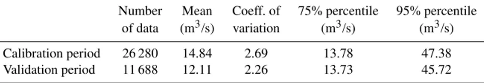
At the closure section, hourly discharge observations [m3/s] were collected between 1 January 1992 and 31 De-cember 1996. For the same observation period, hourly rain-fall depths [mm] at 12 raingauges are available, thus allow-ing the computation of the average areal precipitation over the watershed with an inverse squared distance weighting of the raingauges observations. The calibration procedures de-scribed in the following are based on the continuous data belonging to the first three hydrological years of the obser-vation period, from 1 September 1992 to 31 August 1995. The last 16 months, from 1 September 1995 to 31 December 1996, are used for validation purposes. The main statistics of the streamflow values for the calibration and validation pe-riods are shown in Table 1. The mean and the percentiles are similar, but the variability of the calibration streamflow data is more pronounced than that of the validation data: in particular at the beginning of the calibration period, in au-tumn 1992, occurred the major events (high but nor excep-tional: two peaks with a return period of about 5 years) of the observation period. This is not a drawback for split-sample calibration experiments, but quite the opposite: in fact, the calibration period must have enough information contents, including a wide range of hydrological conditions and in par-ticular it is useful that it includes the highest output values, due to the difficulties ANNs may experience in extrapolation (see, e.g., De Vos and Rientjes, 2008).
Table 1.Statistics of the streamflow observation data sets.
Number Mean Coeff. of 75% percentile 95% percentile of data (m3/s) variation (m3/s) (m3/s)
Calibration period 26 280 14.84 2.69 13.78 47.38
Validation period 11 688 12.11 2.26 13.73 45.72
Forecasting performance measures
The performances of the streamflow forecasting models will be evaluated by the Nash-Sutcliffe efficiency,
EL=1−
P
t=1,N
[Qobs(t+L)−Qsim(t+L)]2
P
t=1,N
[Qobs(t+L)−µobs]2
, L=1÷6, (1)
and through an error measure in the same units of the sim-ulated variable (as suggested also by Legates and McCabe, 1999), namely the mean absolute error,
MAEL= P
t=1,N
|Qobs(t+L)−Qsim(t+L)|
N (2)
wheret is the forecast instant, Qobs and Qsim are the ob-served and simulated streamflow, respectively, µobs is the mean value ofQobs,N is the total number of forecast in-stants andLis the lead-time, varying from one to six hours in the present study.
The efficiency coefficient varies in the range ]–∞, 1], where 1 indicates a perfect agreement and negative values mean that the forecast is worse than assuming future occur-rences equal to the mean valueµobs. The meaningful value of zero provides a convenient reference point to compare the model with the predictive abilities of the observed mean, but the efficiency coefficient, like all the squared measures, tends to inflate the highest errors, that generally correspond to the highest flows. The MAE, on the contrary, gives the same weight to all errors and it is more significant for compar-ing the forecastcompar-ing performances over average and low flow regimes.
As an additional benchmark, the forecasting models will be compared also with a na¨ıve persistent model, where future streamflow is supposed to be equal to the last observed value over all the lead-times:
Qpers(t+L)=Qobs(t ),∀L. (3)
3 Artificial neural networks for streamflow forecasting
The appeal of the use of Artificial Neural Networks (ANNs) as hydrological models lies mainly in their capability to flex-ibly and rapidly reproduce the highly non-linear nature of the
relationship between input and output variables, and it is cer-tainly worthy considering ANN models as powerful tools for real-time short-term runoff forecasts.
An extensive review of the potentiality of ANNs in hy-drological modeling was given, for example, by the ASCE Task Committee (2000b) and by Maier and Dandy (2000). In the majority of the applications of river flow prediction, the networks are fed by both past flows and past precipitation observations: extremely encouraging results have been ob-tained in literature on both real and synthetic rainfall-runoff data (among the many others, in the recent years: Cameron et al., 2002; Solomatine and Dulal, 2003; Jain et al., 2004; Khan and Coulibaly, 2006; Shamseldin et al., 2007; Srivas-tav et al., 2007). Despite the importance of calibration in-formation in a data-driven technique, little attention has been paid, so far, to the influence that the calibration period has on the forecasting performances of ANN rainfall-runoff model-ing. Even if it is acknowledged that the choice of the training set has a fundamental weight (see, for instance, Minns and Hall, 1996; Campolo et al., 1999), only a few studies have presented, so far, an analysis of the impact of the use of dif-ferent training data sets on ANN performances in validation (e.g., Dawson and Wilby, 1998; Anctil et al., 2004; Toth and Brath, 2007). In the proposed approach, different calibration data sets are identified, to be used specifically for modelling the future evolution of similar data.
ANNs distribute computations to processing units called neurons, grouped in layers and densely interconnected. In the
supervisedfeed-forward multilayer networks, three different layer types can be distinguished: an input layer, connecting the input information to the network (and not carrying out any computation), one or more hidden layers, acting as inter-mediate computational layers, and an output layer, producing the final output.
In correspondence of a computational nodeJ, each one of theNj entering values (Ii) is multiplied by a connection weight (wij). Such products are then all summed with a neuron-specific parameter, called bias (bj), used to scale the sum of products into a useful range. The computational node finally applies an activation function (f) to the above sum producing the node output (OJ):
OJ =f (
Nj
X
i=1
The ANNs applied in the present work have only one hidden layer: tan-sigmoidal activation functions were chosen for the hidden layer and linear transfer functions for the output layer. Weights and biases are determined by means of the quasi-Newton Levenberg-Marquardt BackPropagation optimisa-tion procedure (Hagan and Menhaj, 1994), minimising a learning function expressing the closeness between observa-tions and ANN outputs, in the present case the mean squared error. To mitigate overfitting and to improve generalization, a Bayesian regularization of the learning function (Foresee and Hagan, 1997; Anctil et al., 2004) was applied.
For each lead-time, a distinct mono-output network will be implemented: the output of each network,Qsim(t+L), is the streamflow forecast issued, in the forecast instantt, for each lead-timeL.
The input data consist of the most relevant information that is generally available in a real-time flow forecasting system, namely, past rainfall and streamflow observations.
The optimal number of input nodes (corresponding to past streamflow and mean areal precipitation values) and of hid-den nodes to be included in the network is strongly case-dependent. The number of input nodes may be obtained ei-ther with a model-free approach, using statistical measures of dependence (such as correlation or mutual information) to determine the strength of the relationship between candi-date model inputs and the model output, prior to model spec-ification and calibration (e.g., Solomatine and Dulal, 2003; Bowden et al., 2005; Fernando et al., 2009), or with a model based approach, that analyses the performance of models that are calibrated with different inputs, for choosing the most ap-propriate input vector.
In the present work, a model-based approach was used for identifying the dimension of both the input and the hid-den layers: the investigation of the performances of several combinations of input and hidden layers dimensions was per-formed (through a trial-and-error procedure based on a “for-ward selection method”, consisting in beginning by selecting a small number of neurons and then increasing it) in past researches on the same study watershed (partly reported in Toth and Brath, 2007) and will not be described here for sake of brevity. The architecture providing the best trade-off be-tween parsimony and forecasting performances was the one feeding to the input layer four streamflow and three precip-itation values preceding the forecast instant t, Qobs(t−3),
Qobs(t−2), Qobs(t−1), Qobs(t ), P (t−2), P (t−1), P (t ),
with three nodes in the hidden layer and one output node
Qsim (t+L). It was examined the possibility to implement a different architecture for each network, that is for each lead-timeL, but the validation results showed, for eachL, an anal-ogous behaviour when varying the dimension of the layers.
4 Multi-network modeling
Extremely different methods for combining the river flow forecasts issued by a set of different rainfall-runoff mod-els have been recently proposed in the literature, for exam-ple by Shamseldin et al. (1997, 2002, 2007), Abrahart and See (2002), Georgakakos et al. (2004), Solomatine and Siek (2006). This work, in particular, presents an implementation of multiple, alternative models, that is, a modular approach that uses different, specialised rainfall-runoff models, chosen on the basis of the specific hydro-meteorological situation presenting itself in each forecast instant.
precipitation depths is extremely valuable for the identifi-cation of the streamflow evolution: in the period immedi-ately following the forecast, a rising limb, for example, will keep increasing or will reach the peak and begin to decrease depending if the rainfall is continuing or if it has already stopped. Jain and Srinivasulu (2006) used both rainfall and flow values for decomposing the flow hydrograph and then forecasting one-step ahead daily streamflow with a multi-network approach: the decomposition was performed with methods based on physical concepts and with a small SOM network, which classified the flows in low, medium and high ranges. Corzo and Solomatine (2007) applied a modular ar-chitecture based on the distinction of baseflow and excess flow obtained with i) a K-means clustering algorithm, ii) a semi-empirical constant slope method or iii) filtering algo-rithms of the hydrographs (where i) and ii) are again based on past flows only).
The principal difference with the above cited works is that the objective of this study is to forecast the future hourly streamflow not only one-step ahead but for increasing lead-times: to do so it is crucial to identify the conditions of each forecast instant not only in terms of past streamflow data but also of past rainfall data, given the importance of meteoro-logical forcing in the evolution of future, farther flows. It is therefore applied a classification algorithm that is based on both past streamflow and rainfall values, rather than an algorithm that performs a separation of the hydrograph in different rising and falling limbs, based on past streamflow data alone. The present work will thoroughly explore the po-tential of SOMs for identifying the different meteorological and hydrological conditions of each forecasting instant, and therefore the future dominant hydrological processes, for im-proving streamflow forecasts over lead-times from one to six hours.
5 Classification of hydro-meteorological conditions
There are no predefined classes of the conditions character-ising the watershed in each forecast instant: a clustering al-gorithm is here used as anunsupervisedclassifier, where the task is to learn a classification from the data. Such parti-tioning will be based on the most relevant available infor-mation, that is, past rainfall and flow observations, assuming that such variables are able to characterise both the current situation and its near-future evolution. It is important to un-derline that the combination of rainfall and streamflow obser-vations prior to the forecast contains valuable information on the state of saturation of the basin and hence on its capability to respond to recent and current rainfall perturbation. The vector chosen for representing each forecast instant is there-fore the same that will be provided in input to the multilayer feedforward ANNs modelling the future streamflow values.
The classification is based on the use of a SOM (Self Or-ganised Map), which organises the data according to their similarity.
5.1 Self Organising Maps
Self Organising Maps (SOMs), or Kohonen networks (Ko-honen, 1982, 2001), are artificial neural networks of the un-supervised type: as opposite to un-supervised networks (like the multilayer networks introduced in Sect. 3 for rainfall-runoff modelling) there is no known user-defined target that the out-put vector should reproduce: the desired solutions are not given and the network learns to cluster the input data by rec-ognizing different patterns. Unsupervised networks may be viewed as classifiers, where the classes are the clusters that are discovered in the calibration data and new data, such as those of the validation set, may be successively assigned to the same classes.
A SOM is formed by only two layers of nodes: the in-put layer contains a node for each of thenvariables charac-terising the unit to classify and the output layer is an array, generally two-dimensional for the convenience of visual un-derstanding, whose nodes are connected, by weighted con-nections, to the input layer. Each input vector “activates” only one output node (thewinningnode, that will represent its class), using the Kohonen competitive learning rule.
Initially the weights are randomly assigned. When then -dimensional input vector (x) is sent through the network,
each neuron of the network computes a distance measure: a Euclidean distance was here chosen, as in the majority of SOM applications, between the weight (W) and the input:
x−W
=
v u u t
n X
i=1
(xi−Wi)2. (5)
The neuron responding maximally to the given input vector, that is the weight vector having the minimum distance from the input vector, is chosen to be the winning neuron. The winning neuron and its neighbouring neurons are allowed to learn by changing the weights at each training iterationt, in a manner to further reduce the distance between the weights and the input vector:
W (t+1)=W (t )+α(t )hlm(x−W (t )), (6)
whereαis the learning rate,∈[0 1],landmare the positions of the winning and its neighbouring output nodes and hlm is the neighbourhood shape, that reduces the adjustment for increasing distance:
hlm=exp −
l−mk2
2σ (t )2
!
, (7)
The weights of the SOM nodes are adjusted, through the learning process, on the vectors of the calibration set. In the learning process all the calibration input vectors are pro-cessed through the SOM incrementally, one after the other, re-iteratively: for each sample input vectorx, the weights of
the winner node and of the nodes in its neighbourhood are changed closer tox.
Lateral interaction between neighbouring output nodes en-sures that learning is a topology-preserving process in which the network adapts to respond in different locations of the output layer for inputs that differ, while similar input pat-terns activate units that are close together. In this way, a SOM produces a topologically ordered output that displays the similarity between the samples presented to it (Foody, 1999).
At the end of the learning phase, the SOM is used (with-out changing the weights any more) to classify the calibration vectors: the trained network identifies which output node to activate in correspondence of each input vector and all the input vectors that activate the same node belong to the same class. In exactly the same way, the tuned SOM may be used to associate any new vector, such as those of the validation set, to one of the units of the SOM output layer, thus attribut-ing the new data to the clusters identified before.
5.2 SOM-clustering of the hydro-meteorological conditions
The use of a SOM in the proposed research activity en-tails the association of each of the input variables defin-ing the current hydro-meteorological condition,Qobs(t−3),
Qobs(t−2),Qobs(t−1),Qobs(t ),P (t−2),P (t−1),P (t ), to
an input node. In the classification phase, such values are standardised to have mean equal to zero and variance equal to one, in order to give them the same importance in the dis-tance measure.
There is not a predefined number of possible conditions and it was chosen to have an output layer formed by three rows by three columns, for a total of nine nodes, each one corresponding to a class, believing that such number is suffi-cient for representing a variety of hydro-meteorological con-ditions without preventing their following interpretation. The output layer topology is hexagonal, rather than rectangular, so that diagonal neighbours have the same distance as hor-izontal and vertical neighbours, as suggested by Kohonen himself (Kohonen, 2001) and by several works on SOM clus-tering (e.g., Van der Voort et al., 1996; Hsu and Halgamuge, 2003; Shirazi and Menhaj, 2005). The trained network will indicate, for any input vector, the class of the matching fore-cast instant, along with the affinity with other classes.
The SOM was initially applied to the calibration set, that is, to the first three hydrological years of the observation pe-riod, from 1 September 1992 to 31 August 1995. The vectors characterising each one of the instants of such period, for a total of 26 280 records, were iteratively given in input to the
SOM: at the end of the tuning phase, these vectors were clas-sified in nine homogeneous groups, formed by all the vectors resulting assigned to the same node on the output layer.
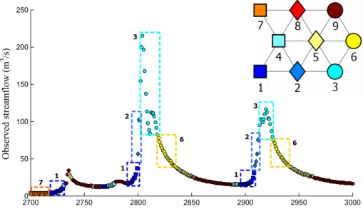
The hexagonal output layer is shown in Fig. 1, using mark-ers that have similar colour and/or shape for the neighbouring nodes. The figure displays also a part of the observed hy-drograph where, at each timet, representing each instant in which a forecast (or better, six forecasts for the varying lead-times) will be issued, the flow value is indicated by a marker having the colour and shape of the class to which the forecast instant is assigned. It is therefore possible to visualise which parts of the hydrograph are associated to the different classes. It should be noted that the hydro-meteorological condition, that is the class, of each forecast instant is the same, inde-pendent of the lead-time that will be successively considered for the forecast.
It may be observed in Fig. 1 that classes 1 and 2 (whose nodes are adjacent on the output layer) correspond to the ris-ing limbs (beginnris-ing of the risris-ing for class 1, values closer to the peak for class 2), whereas nodes 3 and 6 (contiguous as well, even if diagonally, on the hexagonal map) correspond to the maximum flow values, respectively around the peak and at the beginning of the falling limb. Nodes 7 and 8, even if it is less evident in the hydrograph zoom reported in the figure, are associated to recession low flows. The hydro-meteorological conditions corresponding to the remaining nodes (4, 5 and 9) are instead intermediate between the pre-viously described classes and less easily identifiable.
The nature of the various classes pictured in Fig. 1 is recognisable also by analysing their size and the mean values of the different variables in each class, reported in Table 2.
The table highlights that classes 1 and 2 are characterised by the highest precipitation values, as expectable along rising limbs, while the highest streamflow values are associated to nodes 3 and 6. Minimum streamflow values and precipitation practically null are associated to nodes 7 and 8 and it may also be noted that such conditions are largely dominant in terms of class occupancy.
Overall, the SOM seems to be able to clearly recognize the different conditions, distinguishing the parts of the hy-drograph not only in terms of the flow value observed in the forecast instant and in the previous ones, but taking into ac-count also the recent meteorological forcing: such distinction may be advantageous for discerning the near-future trend of the hydrograph evolution.
27000 2750 2800 2850 2900 2950 3000 50
100 150 200 250
Idrogramma
Time (hours, from 1 September 1992, 0:00) 7
1
1 2
2 3
3
6
6
1
O
b
se
rved st
re
am
fl
o
w
(m
3 /s
)
Fig. 1. Markers associated to the SOM output layer nodes (upper right-hand corner) and part of the observed hydrograph: the streamflow value relative to each forecast instant is indicated with the marker of the corresponding class. The elements belonging to classes 1, 2, 3, 6, and 7 are put in evidence by the dotted boxes of the matching colours.
Table 2.Size of the nine classes obtained with the SOM and mean values, for each class, of the variables forming the input vectors of the calibration set.
Mean value
Class Class Qt Qt−1 Qt−2 Qt−3 Pt Pt−1 Pt−2
size (m3/s) (m3/s) (m3/s) (m3/s) (mm/h) (mm/h) (mm/h)
1 1141 9.11 8.50 8.14 7.92 1.84 1.81 1.62
2 329 46.40 41.36 38.52 37.02 1.19 1.54 1.64
3 602 215.13 216.42 215.78 213.80 0.73 0.80 0.89
4 1295 5.87 5.79 5.74 5.69 0.28 0.23 0.29
5 1403 30.68 30.77 30.90 31.10 0.13 0.11 0.12
6 940 54.86 55.97 57.04 58.07 0.07 0.06 0.07
7 12 166 2.13 2.14 2.15 2.15 0.00 0.00 0.00
8 5462 9.09 9.12 9.16 9.20 0.01 0.00 0.01
9 2942 19.38 19.47 19.58 19.72 0.02 0.01 0.02
phase (as will be confirmed by the forecasting results on val-idation data described in Sect. 6).
To overcome this problem, the opportunity to form wider classes of observations (but always homogeneous from a hy-drological point of view) was tested, so to ensure a greater size of the data sets used in the calibration procedure.
Partitioning of the hydro-meteorological conditions in wider classes
The SOM classification offers a straightforward solution for the identification of similar classes, which may be joined to form broader, homogeneous groups of data. In fact, as said in Sect. 5.1, input vectors belonging to similar classes
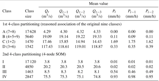
Table 3.Class size and mean values of the variables forming the input vectors of the calibration set for the two 4-class partitionings.
Mean value
Class Class Qt Qt−1 Qt−2 Qt−3 Pt Pt−1 Pt−2
size (m3/s) (m3/s) (m3/s) (m3/s) (mm/h) (mm/h) (mm/h)
1st 4-class partitioning (reasoned association of the original nine classes)
A (7+8) 17 628 4.29 4.30 4.32 4.33 0.00 0.00 0.00
B (4+5+9) 5640 19.09 19.14 19.22 19.33 0.11 0.09 0.11
C (1+2) 1470 17.46 15.85 14.94 14.43 1.69 1.75 1.62
D (3+6) 1542 117.43 118.61 119.01 118.87 0.33 0.35 0.39
2nd 4-class partitioning (4-node SOM)
I 17 120 3.8 3.8 3.8 3.8 0.01 0.01 0.01
II 4850 20.2 20.3 20.5 20.6 0.02 0.02 0.02
III 1463 8.5 8.3 8.2 8.1 0.54 0.46 0.49
IV 2847 75.5 75.3 75.1 74.8 0.93 0.98 0.95
The four classes resulting from this reasoned association of the original classes may be compared with those that are obtainable setting up a new SOM, with only four nodes in the output layer, thus getting a second partitioning of the data in four classes.
The properties of these two 4-class partitionings of the cal-ibration data are reported in Table 3.
The classes identified automatically by the 4-node SOM and those obtained by the reasoned associations (here named with letters) of the nodes of the original 9-node SOM do not coincide: in particular, the 4-node SOM does not seem able to clearly identify the cluster of the rising limbs, charac-terised by the highest rainfall (classes 1 and 2 of the 9-node SOM, joined in one class, named class C, in the reasoned as-sociated classes) and to distinguish it from the data that are around the peak and at the beginning of falling limbs (classes 3 and 6 of the 9-node SOM, joined in class D). The approach for obtaining wider classes that is based on the topological properties of the original SOM appears therefore more suit-able for the preservation of the hydrological distinctiveness of the classes.
6 Rainfall-runoff modelling
Preliminary to the design of the modular approaches, in order to have a term of comparison for the multi-network results, one traditional, global rainfall-runoff ANN model is imple-mented, trained on all the data belonging to the calibration period. As a matter of fact, as described in Sect. 3, six dif-ferent mono-output feed-forward networks, with seven nodes in the input layer and three hidden nodes, were implemented for forecasting the future streamflow from one to six hours ahead,Qsim(t+L).
Having identified, in Sect. 5, the nature of the differ-ent hydro-meteorological conditions and the corresponding classes of forecast instants, it is then possible to build the modular rainfall-runoff systems.
The first modular approach is built on the basis of the 9-class partitioning: nine different rainfall-runoff ANN models are implemented, each one formed by six mono-output net-works for the varying lead-times. Every model is parame-terised through a training procedure that uses exclusively the input-output vectors, of the calibration period, belonging to the same class. In this way, a different model is built for each class, to be used for each particular hydro-meteorological condition.
In the validation phase, streamflow forecasts are issued in correspondence of every hour belonging to the last 16 months of the observation period, whose data was not used in any way in the tuning of the SOM, nor in the parameterisation of the rainfall-runoff models. In the modular approach, the tuned SOM already used to classify the calibration data is first used to associate every forecast instant of the valida-tion period to one of the identified nine classes. The rainfall-runoff module representing that class is then chosen for issu-ing the streamflow forecasts.
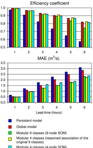
The goodness-of-fit measures of the validation forecasts that are presented in Fig. 2 indicate, as expected, a remark-able improvement for both the global model (red bars) and the 9-class modular one (green bars) in comparison with the simple persistent model (blue bars). It is, on the other hand, evident that the use of the 9-module model allows an im-provement of the MAE index, but it entails a deterioration of the efficiency coefficients, if compared to the global model.
Efficiency coefficient 0.5 0.6 0.7 0.8 0.9 1.0
1 2 3 4 5 6
MAE (m3/s)
0.0 0.5 1.0 1.5 2.0 2.5 3.0 3.5
1 2 3 4 5 6 Lead-time (hours)
Persistent model
Global model
Modular 9 classes (9-node SOM)
Modular 4 classes (reasoned association of the original 9 classes)
Modular 4 classes (4-node SOM)
Fig. 2.Performance measures of streamflow forecasts for the vali-dation data set.
of the insufficient informative content of the calibration data. This inadequacy is likely to affect the classes different from 7 and 8, which, in addition to be the most numerous, are also those associated to the lowest streamflow values: it follows that less reliable performances may be expected in the pre-diction of the higher flows. Since the efficiency coefficient amplifies the highest errors, which generally coincide with the highest flows, this would justify the deterioration of such coefficient for the 9-class modular model.
Two additional modular approaches were then imple-mented, based on the 4-class partitionings that were iden-tified in Sect. 5.2, whose classes are more numerous.
The second modular system is based on the four classes obtained from the association (on the basis of their simi-larity) of the original nine classes. Four different rainfall-runoff network models are calibrated using all and only the data belonging to each one of the four classes of hydro-meteorological conditions. Figure 3 shows the 1 to 6 h ahead forecasts issued by this approach in correspondence of dif-ferent forecast instants (blue diamonds) for three validation events: the behaviour, even if somewhere fluctuating (as ex-pectable since the forecasts are issued by independent mod-els), is not too unrealistic.
0 50 100 150 200 250 300 350 400 450
0 6 12 18 24 30 36 42 48
Hours (from 26 December 1995, 8:00)
Streamfl ow (m 3/s) 0 2 4 6 8 10 12 14 16 18 20 Prec ip it at io n (mm/h) 0 50 100 150 200 250 300 350 400 450
0 6 12 18 24 30 36 42 48
Hours (from 7 January 1996, 0:00)
Streamflow (m 3/s) 0 2 4 6 8 10 12 14 16 18 20 Prec ip it at ion (mm /h) 0 50 100 150 200 250 300 350 400 450
0 6 12 18 24 30 36 42 48
Hours (from 17 February 1996, 22:00)
Streamfl ow (m 3/s) 0 2 4 6 8 10 12 14 16 18 20 Prec ip it at io n (mm/h)
Precipitation Qobs Forecast instant
LT=1 hour LT=2 hours LT=3 hours
LT=4 hour LT=5 hours LT=6 hours
Fig. 3. Observed hydrographs (Qobs) for three validation events and, in correspondence of different forecast instants, the forecasts (for lead-times LT=1÷6 h) issued by the modular approach based on the reasoned association of the original 9 classes.
In analogous way, the third, and last, forecasting modular approach was implemented on the basis of the classes auto-matically identified by the 4-node SOM.
but are analogous, or even slightly worse, for the shortest lead-times. This is probably due to the fact that for short lead-times, due to the response time of the watershed, there is less influence of the most recent rainfall values: such val-ues will instead control the evolution of the phenomena over longer time horizons, especially for the highest flow values. Therefore, for short lead-times, also the global model may allow satisfactory efficiencies, whereas, for longer time hori-zons, differentiating the hydro-meteorological conditions be-comes crucial.
The forecasts issued by the 4-class modular approach whose classes are formed by the reasoned associations of the nine original classes are always better, especially as far as the MAE index is concerned, than those based on the 4-node SOM. This is to be ascribed to the fact that, as said in Sect. 5.2, the groups obtained from the similarity of the original classes seem able to better preserve the distinctive features of the hydro-meteorological conditions.
Overall, the modular approach based on the four, wider classes obtained on the basis of the affinity among the char-acterising hydro-meteorological conditions appears the best performing one, especially for the longest lead-times.
7 Conclusions
The SOM method has proved to be an instrument suit-able for an objective, automatic classification of the hydro-meteorological conditions of the watershed: its use allowed in fact a satisfactory identification of the different parts of the hydrograph representing current and near-future hydrologi-cal conditions, on the basis of the most relevant information available in the forecast instant, that is recent streamflow and rainfall observations.
As far as the real-time rainfall-runoff modelling is con-cerned, the performances of the first modular approach, based on nine classes of hydro-meteorological situations, appear penalised by the low occupancy of some of the classes. The reduced informative content of not sufficiently numerous classes may in fact prevent an adequate char-acterisation of the input-output relationship in the calibra-tion phase. Broader classes were therefore formed, through an association of the clusters representing similar hydro-meteorological conditions, exploiting the property of the SOM, unique among the other clustering techniques, to pro-vide indications on the similarity between the classes. The new modular system, differentiating the rainfall-runoff mod-els according to classes that are wider but still preserve the hydrological distinctiveness of the hydro-meteorological conditions, allowed a remarkable improvement of the per-formances in validation, in comparison to both the 9-class modular approach and to the global one. Such finding high-lights the important influence, on the streamflow forecasts, of the number and properties of the classes that are identified by the SOM: additional research on this aspect will be the topic of future work.
Overall, the results show that an adequate distinction of the hydro-meteorological conditions that characterise the basin at the forecast instant, thus including additional knowledge on the forthcoming hydrological processes, may consider-ably improve the rainfall-runoff modelling performance. Acknowledgements. The author wishes to thank E. Zehe, D. Solo-matine, U. Ehret and an Anonymous Referee for their constructive and helpful comments, which certainly enhanced the quality and readability of the paper.
Edited by: E Zehe
References
Abrahart, R. J. and See, L.: Comparing neural network and autore-gressive moving average techniques for the provision of contin-uous river flow forecasts in two contrasting catchments, Hydrol. Process., 14(11), 2157–2172, 2000.
Abrahart, R. J. and See, L.: Multi-model data fusion for river flow forecasting: an evaluation of six alternative methods based on two contrasting catchments, Hydrol. Earth Syst. Sci., 6, 655–670, 2002, http://www.hydrol-earth-syst-sci.net/6/655/2002/. Anctil, F., Perrin, Ch., and Andreassian V.: Impact of the length of
observed records on the performance of ANN and of conceptual parsimonious rainfall-runoff forecasting models, Environ. Mod-ell. Softw., 19, 357–368, 2004.
ASCE Task Committee on Application of Artificial Neural Net-works in Hydrology: Artificial neural netNet-works in hydrology. I: preliminary concepts, J. Hydrol. Eng., 5, 115–123, 2000a. ASCE Task Committee on Application of Artificial Neural
Net-works in Hydrology: Artificial neural netNet-works in hydrology II: hydrologic applications, J. Hydrol. Eng., 5, 124–137, 2000b. Astel, A., Tsakovski, S., Barbieri, P., and Simeonov, V.:
Compari-son of self-organizing maps classification approach with cluster and principal components analysis for large environmental data sets, Water Res., 41(19), 4566–4578, 2007.
Bowden, G. J., Dandy G. C., and Maier, H. R.: Input determination for neural network models in water resources applications. Part 1 – background and methodology, J. Hydrol., 301, 75–92, 2005 Cameron, D., Kneale, P., and See, L.: An evaluation of a traditional
and a neural net modelling approach to flood forecasting for an upland catchment, Hydrol. Process., 16, 1033–1046, 2002. Campolo, M., Andreussi, P., and Soldati, A.: River flood
forecast-ing with neural network model, Water Resour. Res., 35(4), 1191– 1197, 1999.
Corzo, G. A. and Solomatine, D. P.: Baseflow separation techniques for modular artificial neural networks modelling in flow forecast-ing, Hydrolog. Sci. J., 52(3), 491–507, 2007.
Coulibaly, P., Bob´ee, B., and Anctil, F.: Improving extreme hydro-logic events forecasting using a new criterion for artificial neural network selection, Hydrol. Process., 15, 1533–1536, 2001. Dawson, C. W. and Wilby, R.: An artificial neural network
ap-proach to rainfall-runoff modeling, Hydrolog. Sci. J., 43(1), 47– 65, 1998.
de Vos, N. J. and Rientjes, T. H. M.: Multiobjective training of artifi-cial neural networks for rainfall-runoff modeling, Water Resour. Res., 44, W08434, doi:10.1029/2007WR006734, 2008. Fernando, T. M. K. G., Maier, H. R., and Dandy, G. C.: Selection
of input variables for data driven models: An average shifted histogram partial mutual information estimator approach, J. Hy-drol., 367, 165–176, 2009.
Foody, G.: Applications of the self-organising feature map neural network in community data analysis, Ecol. Model., 120, 97–107, 1999.
Foresee, F. D. and Hagan, M. T.: Gauss-Newton approximation to Bayesian learning, IEEE IJCNN, New York, 3, 1930–1935, 1997.
Furundzic, D.: Application example of neural networks for time series analysis: rainfall-runoff modelling, Signal Process., 64, 383–396, 1998.
Georgakakos, K. P., Seo, D., Gupta, H., Schaake, J., and Butts, M. B.: Towards the characterization of streamflow simulation uncer-tainty through multimodel ensembles, J. Hydrol., 298, 222–241, 2004.
Gopakumar R., Takara, K., and James E. J.: Hydrologic Data Ex-ploration and River Flow Forecasting of a Humid Tropical River Basin Using Artificial Neural Networks, Water Resour. Manag., 21(11), 1915–1940, 2007.
Gupta, H. V., Sorooshian, S., and Yapo, P. O.: Toward improved calibration of hydrologic models: Multiple and noncommensu-rable measures of information, Water Resour. Res., 34, 751–764, 1998.
Hagan, M. T. and Menhaj, M.: Training feedforward networks with the Marquardt algorithm, IEEE T. Neural Networ., 5(6), 989– 993, 1994.
Hsu, A. L. and Halgamuge, S. K.: An unsupervised hierarchical dynamic selforganizing approach to cancer class discovery and marker gene identification in microarray data (supplementary in-formation on “Dynamic SOM with hexagonal structure for data mining”), Bioinformatics, 19(16), 2131–2140, 2003.
Hsu, K., Gupta, H. V., Gao, X., Sorooshian, S., and Imam, B.: Self-organizing linear output map (SOLO): An artificial neural net-work suitable for hydrologic modeling and analysis, Water Re-sour. Res., 38(12), 1302, doi:10.1029/2001WR000795, 2002. Jain, A., Sudheer, K. P., and Srinivasulu, S.: Identification of
phys-ical processes inherent in artificial neural network rainfall runoff models, Hydrol. Process., 18, 571–581, 2004.
Jain, A. and Srinivasulu, S.: Integrated approach to model decom-posed flow hydrograph using artificial neural network and con-ceptual techniques, J. Hydrol., 317, 291–306, 2006.
Kalteh, A. M., Hjorth, P., and Berndtsson, R.: Review of the self-organizing map (SOM) approach in water resources: Analysis, modelling and application, Environ. Modell. Softw. 23, 835–845, 2008.
Khan, M. S. and Coulibaly, P.: Bayesian neural network for rainfall-runoff modeling, Water Resour. Res., 42(7), W07409, doi:10.1029/2005WR003971, 2006.
Kohonen, T.: Self-organized formation of topologically correct fea-ture maps, Biol. Cybern., 43, 59–69, 1982.
Kohonen, T.: Self-Organizing Maps (third edn.), Springer, Berlin, Germany, 2001.
Legates, D.R. and McCabe, G.J.: Evaluating the use of ‘goodness-of-fit’ measures in hydrologic and hydroclimatic model
valida-tion, Water Resour. Res., 35, 233-241, 1999.
Madsen, H.: Automatic calibration of a conceptual rainfall-runoff model using multiple objectives, J. Hydrol., 235, 267–288, 2000. Maier, H. and Dandy, G.: Neural networks for the prediction and forecasting of water resources variables: A review of modeling issues and applications, Environ. Modell. Softw., 15(1), 101– 104, 2000.
Mangiameli, P., Chen, S. K., and West, D.: A comparison of SOM neural network and hierarchical clustering methods, Eur. J. Oper. Res., 93, 402–417, 1996.
Minns, A. W. and Hall, M. J.: Artificial neural networks as rainfall runoff models, Hydrolog. Sci. J., 41, 399–417, 1996.
Moradkhani, H., Hsu, K., Gupta, H. V., and Sorooshian, S: Im-proved streamflow forecasting using self-organizing radial ba-sis function artificial neural networks, J. Hydrol., 295, 246–262, 2004.
Parasuraman, K. and Elshorbagy, A.: Cluster-based hydrologic pre-diction using genetic-algorithm trained neural networks, J. Hy-drol. Eng., 12(1), 52–62, 2007.
Shamseldin, A. Y., Nasr, A. E., and O’Connor, K. M.: Comparison of different forms of the Multi-layer Feed-Forward Neural Net-work method used for river flow forecasting, Hydrol. Earth Syst. Sci., 6, 671–684, 2002,
http://www.hydrol-earth-syst-sci.net/6/671/2002/.
Shamseldin, A. Y., O’Connor, K. M., and Liang, G. C.,: Methods for combining the outputs of different rainfall-runoff rodels, J. Hydrol., 197, 203–229, 1997.
Shamseldin, A. Y., O’Connor, K. M., and Nasr, A. E.: A compara-tive study of three neural network forecast combination methods for simulated river flows of different rainfall-runoff models, Hy-drolog. Sci. J., 52(5), 896–916, 2007. natural phenomena, Neural Networks, 19, 215–224, 2006.
Shirazi, J. and Menhaj, M. B.: A SOM Based 2500-Isolated-Farsi-Word Speech Recognizer, in: ICANN 2005, LNCS 3696, edited by: Duch, W., Kacprzyk, J., Oja, E., and Zadrony, S., Springer-Verlag Berlin Heidelberg, 589–595, 2005.
Solomatine, D. P. and Siek, M. B.: Modular learning models in forecasting
Solomatine, D. P. and Dulal, K. N.: Model trees as an alternative to neural networks in rainfall-runoff modelling, Hydrolog. Sci. J., 48(3), 399–411, 2003.
Srivastav, R. K., Sudheer, K. P., and Chaubey, I.: A simplified ap-proach to quantifying predictive and parametric uncertainty in artificial neural network hydrologic models, Water Resour. Res., 23(10), W10407, doi:10.1029/2006WR005352, 2007.
Tang, Y., Reed, P., and Wagener, T.: How effective and efficient are multiobjective evolutionary algorithms at hydrologic model calibration?, Hydrol. Earth Syst. Sci., 10, 289–307, 2006, http://www.hydrol-earth-syst-sci.net/10/289/2006/.
Toth, E. and Brath, A.: Multistep ahead streamflow fore-casting: Role of calibration data in conceptual and neu-ral network modeling, Water Resour. Res., 43, W11405, doi:10.1029/2006WR005383, 2007.
Van der Voort, M., Dougherty, M., and Watson, S.: Combining Ko-honen maps with ARIMA time series models to forecast traffic flow, Transport. Res., C4(5), 307–318, 1996.
1–19, 2003.
Wang, W., Gelder, P., Vrijling, J. K., and Ma, J.: Forecasting daily streamflow using hybrid ANN models, J. Hydrol., 324(1), 383– 399, 2006.
Wheater, H. S., Jakeman, A. J., and Beven, K. J.: Progress and directions in rainfall-runoff modelling, in: Modelling change in environmental systems, edited by: Jakeman, A. J., Beck, M. B., and McAleer, M. J., Wiley, Chichester, 101–132, 1993.
World Meteorological Organization: Simulated real-time intercom-parison of hydrological models, WMO Publications, Geneva, Swiss, 1992.
Young, P. C.: Advances in real-time flood forecasting, Philos. T. R. Soc. Lond., 360, 1433–1450, 2002.