Ann. Geophys., 30, 597–611, 2012 www.ann-geophys.net/30/597/2012/ doi:10.5194/angeo-30-597-2012
© Author(s) 2012. CC Attribution 3.0 License.
Annales
Geophysicae
Study of the applicability of the curlometer technique with the four
Cluster spacecraft in regions close to Earth
S. Grimald1,2, I. Dandouras1,2, P. Robert3, and E. Lucek4
1Universit´e de Toulouse, UPS-OMP, UMR5277, Institut de Recherche en Astrophysique et Plan´etologie, Toulouse, France 2CNRS, Institut de Recherche en Astrophysique et Plan´etologie, Toulouse, France
3Laboratoire de Physique des Plasmas, CNRS, Paris, France 4Blackett Laboratory, Imperial College, London, UK
Correspondence to:S. Grimald ([email protected])
Received: 24 June 2011 – Revised: 14 February 2012 – Accepted: 17 February 2012 – Published: 27 March 2012
Abstract. Knowledge of the inner magnetospheric current system (intensity, boundaries, evolution) is one of the key el-ements for the understanding of the whole magnetospheric current system. In particular, the calculation of the current density and the study of the changes in the ring current is an active field of research as it is a good proxy for the mag-netic activity. The curlometer technique allows the current density to be calculated from the magnetic field measured at four different positions inside a given current sheet using the Maxwell-Ampere’s law. In 2009, the CLUSTER perigee pass was located at about 2REallowing a study of the ring
current deep inside the inner magnetosphere, where the pres-sure gradient is expected to invert direction. In this paper, we use the curlometer in such an orbit. As the method has never been used so deep inside the inner magnetosphere, this study is a test of the curlometer in a part of the magneto-sphere where the magnetic field is very high (about 4000 nT) and changes over small distances (1B=1 nT in 1000 km). To do so, the curlometer has been applied to calculate the current density from measured and modelled magnetic fields and for different sizes of the tetrahedron. The results show that the current density cannot be calculated using the cur-lometer technique at low altitude perigee passes, but that the method may be accurate in a [3RE; 5RE] or a [6RE; 8.3RE]
L-shell range. It also demonstrates that the parameters used to estimate the accuracy of the method are necessary, but not sufficient conditions.
Keywords. Magnetospheric physics (Current systems)
1 Introduction
The existence of a current circling the Earth in the near Earth region was first suggested by Singer (1957). The ring current can be visualized as a toro¨ıdal ring current flowing around the Earth at geocentric distances from 2REto 9RE (where
REis the Earth radius). Two phenomena are responsible for
the existence of a current at this position: first, the gradient drift of particles above about 1 keV which produces a west-ward current and, second, the magnetisation current whose direction depends on the direction of the particle pressure gradient. Studies of the particle pressure in the inner magne-tosphere show that the direction of its gradient changes when travelling in the ring current: it is directed outwards close to the Earth and in the opposite direction (inward) far from it (Lui et al., 1987, Lui and Hamilton, 1992). These observa-tions indicate that two ring currents exist: an eastward one, below a given altitude, and a westward one, above it. This effect had been observed in satellite data (see Le et al., 2004; Jorgensen et al., 2004) and the current reversal boundary had been located between 3REand 4RE.
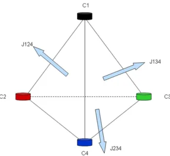
Fig. 1. Illustration of the average current density estimation using the curlometer (adapted from Dunlop et al., 1988).
energy/time spectrograms of the particles. It is well known that the ring current evolution depends, first, on the parti-cle injections during increasing of the magnetic activity and, second, on the loss mechanisms (Daglis et al., 1999), but the current driven by this population as well as the position of the reversal boundary remain to be determined. One way to find it is to estimate the current density.
Two methods have been developed in order to calculate the current density: the method of the pressure gradient, which uses the plasma fluid momentum equation (Lui et al., 1987; Roelof et al., 2004), and the curlometer technique, which uses the Maxwell-Ampere law (Robert and Roux, 1993; Robert et al., 1998a; Dunlop et al., 2002; Dunlop and Balogh, 1993). The first method requires the determination of pres-sure gradients, which is quite difficult using satellite data. The second method requires magnetic field measurements at different points inside the current sheet. The four satellites of the Cluster mission cross the ring current at different po-sitions in their orbits. Their magnetic field data have been used by Vallat et al. (2005) to calculate the current density for different events observed in 2002, when the Cluster perigee was located at 4RE. This position of the perigee pass
al-lowed the study of the westward ring current, the partial one and the inner plasmasheet, which brought new results about the latitudinal extent of the ring current and the dependence of its intensity on the magnetic activity in the evening sec-tor. Since 2009, the Cluster perigee altitude has decreased to about 2RE. As a consequence, the orbit crosses the
re-gion where the current reversal boundary, as defined by Le at al. (2004) and by Jorgensen et al. (2004), is expected. A study of the current density along such an orbit could give us a better knowledge of the current density deeper inside the
inner magnetosphere than ever calculated before, but could also provide a more precise location of the reversal bound-ary. Here, we use the curlometer technique to study the ring current for ring current crossings observed in 2009. As the curlometer has never been used so deep inside the in-ner magnetosphere, this study is also a test of the curlometer in a part of the magnetosphere where the magnetic field is very high (about 4000 nT) and varies over small distances (1B=1 nT in 1000 km). Section 2 presents briefly the cur-lometer technique. Section 3 presents the 15 May 2009 ring current crossing and the results from the curlometer for this event. Sections 4 and 5 present a test of the curlometer along the 15 May 2009 orbit and for different separations. Conclu-sions are given in Sect. 6.
2 The curlometer technique
The curlometer technique has been described by Dunlop et al. (1988, 2002), Chanteur and Mottez (1993) and Robert et al. (1998a). It uses the Maxwell-Ampere’s law to esti-mate the current density J through the tetrahedron formed by four spacecraft. This section gives a quick description of the method.
2.1 Basic definitions
Assuming stationarity in the studied medium, the Maxwell-Ampere’s law can be written as:
µ0J=cur lB (1)
Using four spacecraft travelling together in a tetrahedral con-figuration (see Fig. 1), it is possible to determine the average current density normal to each face of the tetrahedron. As-suming the current density is a constant in the whole surface and the magnetic field changes very slowly, relation (1) can be written as (Dunlop et al., 1988):
µ0Jij k.(1rik×1rj k)=1Bik.1rj k−1Bj k.1rik (2) Wherei,j andk refer to the satellite number, Jij k is the
average current density normal to the surface made by the satellitesi,j andk,1rik =ri−rk is the distance between the satelliteiand the satellitej, and1Bik=Bi−Bk is the magnetic field difference between the satelliteiand the satel-litej. As an example, J123 is the average current density normal to the surface formed by C1, C2 and C3 (see Fig. 1). Using relation (2):
µ0J123.(1r13×1r23)=1B13.1r23−1B23.1r13
S. Grimald et al.: Study of the applicability of the curlometer technique 599
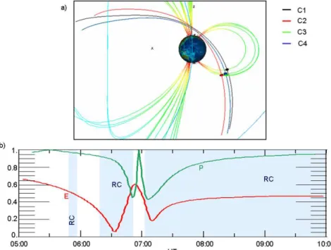
Fig. 2. (a)orbit of the four Cluster satellites for the 15 May 2009 ring current crossings. The colour code refers to the various satellites (black is C1, red is C2, green is C3 and blue is C4). The configuration of the tetrahedron at 06:00 UT can be seen in(a).(b)elongationE(in red) and planarityP (in green) of the tetrahedron. The blue shaded areas indicate the time intervals when the ring current is observed in C1 data.
Fig. 3.Evolution of the magnetic field measured by the FGM instrument on board the four satellites. The colour code refers to the various satellites (black is C1, red is C2, green is C3 and blue is C4).
2.2 Accuracy of the method
The error sources of the curlometer have been studied by Dunlop et al. (2002), Chanteur (1998) and Robert et al. (1998a) and summarized by Vallat et al. (2005). They come from the assumptions made to obtain relation (2) and the usage of four separated satellites.
First, the two main assumptions of this technique are the linear variation of the magnetic field so thatJav is constant over the tetrahedron and the stationarity over the studied cur-rent sheet. As the non-stationarity of the medium leads to the generation of nonlinear gradients in the magnetic field, the only point to check here is the linear variation of the mag-netic field. To do so, Dunlop et al. (1988) showed that it is possible to calculate an estimate for divBfrom:
divB1rik.1rj k×1rj l =
X
cyclic
1Bik. 1rj k×1rj l
(3)
It is well known thatBis solenoidal (Maxwell-Thomson
is dimensionless and as it depends on the difference between the magnitude of divB andcur l B. It has been stated that divB
cur l B≪1 indicates a good estimate of the average current density whereas divB
cur l B≥1 indicates a stan-dard deviation higher than 100 %.
Second, the magnetic field is measured by four satel-lites forming a tetrahedron, which can have many different shapes. It has been shown by Robert et al. (1998a) that only particular shapes can lead to the calculation of theJav. The size of the tetrahedron has to be small enough so as to per-mit the gradients (inside the tetrahedron) to be as linear as possible. However, the smaller the tetrahedron is, the larger the absolute error made on1Band1restimation is, and the more important the resulting error onJavis too. Moreover, a
too elongated or a too planar tetrahedron will lead to impor-tant errors on the estimation of some of theJavcomponents
and will decrease the accuracy of the method.
3 Event presentation
3.1 Cluster orbit and instrumentation
The Cluster mission is based on four identical spacecraft (de-noted C1, C2, C3 and C4) launched on similar elliptical polar orbits. Figure 2a presents the orbit of the four Cluster satel-lites for the 15 May 2009 ring current crossings. The colour code refers to the various satellites (black is C1, red is C2, green is C3 and blue is C4). The magnetic equator is crossed at 06:29 UT (C1), 06:33 UT (C2 and C4) and 06:35 UT (C3). At the beginning of the mission, the perigee was at 4REand
the apogee at 19.6RE (Escoubet et al., 2001). Due to
or-bital perturbations and drag from the exosphere, the perigee decreases slowly and it was about 2RE during the time
in-terval under study. The configuration of the tetrahedron at 06:00 UT can be seen in Fig. 2a. The four Cluster satellites had a separation of 1000 km when crossing the auroral zone area. C1 was leading and then came C2, C4 and C3 brings up the rear. The shape of the tetrahedron evolves along the trajectory of the spacecraft. To characterise the geometrical shape of the tetrahedron during the time interval under study, Fig. 2b presents the elongationE(in red) and the planarityP
(in green) of the tetrahedron between 05:00 UT and 10:00 UT (see Robert et al., 1998b, for a definition of these two fac-tors). EandP lie between 0 and 1. As shown by Robert et al. (1998b),E=1 means the four satellites are located along a straight line whateverP is (1-D tetrahedron),P=1 means the four satellites are located in a plane whateverEis (2-D tetrahedron), andE=0 means the satellites are located in the circumference of a circle ifP=1 (2-D tetrahedron) and of a sphere ifP=0. As shown in Fig. 2b,Evaries between 0.05 and 0.6 during the whole observation whenP lies between 0.4 and 1. As a consequence, the satellites are located in the surface of a more or less elongated ellipsoid, and in a plane at 05:30 UT and 06:57 UT.
Eleven experiments on board each spacecraft allow a wide variety of measurements of the plasma parameters (particles and fields). Among them, a fluxgate magnetometer (FGM), as well as two ion spectrometers (HIA and CODIF), are present. We will now present the data of these two instru-ments for the ring current crossings under study as well as the geomagnetic activity level.
3.2 FGM data and geomagnetic activity
The FGM experiment on board Cluster consists of two triax-ial fluxgate magnetometers and an onboard data-processing unit on each spacecraft (Balogh et al., 1997, 2001). High vector sample rates (up to 67 vectors s−1) at high resolution (up to 8 pT) allow for a precise measurement of the ambient magnetic field. The background interference from the space-craft is minimised by the positioning of the magnetometers on a five metre boom, which avoids interference from the spacecraft. The magnetic field component along the spin axis (which is almost perpendicular to the ecliptic) will carry the main part of the error made on the measurement, because offsets in the spin plane measurements are easily removed by noting spin-period oscillations. In addition to the on-ground calibrations made to determine the expected maximal offset on each spacecraft (up to 0.1 nT), in-flight calibrations of the magnetometers are regularly applied in order to maximise the accuracy of the magnetic field measurements.
Figure 3 presents the evolution of the magnetic field mea-sured by the FGM instrument on board the four satellites between 04:00 UT and 13:00 UT. As shown in Fig. 2a, the satellites cross the inner magnetosphere from the Southern Hemisphere to the northern one. During the orbit, the mag-netic field measured on board each satellite increases reach-ing a maximum in the cusp region (Fig. 3). Afterwards, the magnetic field decrease when the satellites travel toward the night side.
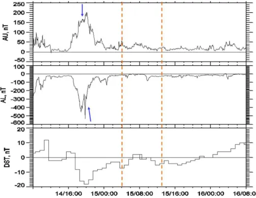
Figure 4 presents the AU (top panel), AL (middle panel) and Dst (bottom panel) indices evolution between the 14 May 2009 at 08:00 UT and the 16 May 2009 at 08:00 UT. The orange dashed lines are located 04:00 UT and at 13:00 UT and delimitate the time range of the magnetic field data presented in Fig. 3. A variation of the auroral in-dices is observed before the observation (blue arrows). As a reminder, the AU index measures the intensity of the east-ward electrojet which is part of the region 2 current system, while the AL index measures the intensity of the westward electrojet which is part of the region 1 current system. The region 2 current system closes in the night side, close to the magnetic equator atL≈4RE. The region 1 current system
S. Grimald et al.: Study of the applicability of the curlometer technique 601
Fig. 4.AE (top panel), AU (middle panel) and Dst (bottom panel) indices evolution between the 14 May at 08:00 UT and the 16 May 2009 at 08:00 UT. The orange dashed lines are located on 15 May at 04:00 UT and at 13:00 UT and delimitate the time range of the magnetic field data presented in Fig. 3. The blue arrows indicate variations of the auroral indices.
only very slightly disturbed by the injection of particles and the magnetic field compression. To summarize, variations in the solar wind are responsible for the injection of particles and the compression of the magnetosphere, but they are weak enough to cause no more than a very low disturbance of the ring current.
3.3 CIS data
The Cluster Ion Spectrometer experiment consists of two complementary ion sensors, the COmposition and Distribu-tion FuncDistribu-tion analyzer (CODIF) and the Hot Ion Analyzer (HIA). CODIF gives a mass per charge composition with a 22.5◦angular resolution and HIA offers a better angular res-olution (∼5◦), but without mass discrimination. CIS is capa-ble of measuring the full three-dimensional ion distribution of the major ion species, from thermal energies (∼1 eV q−1) to about 40 keV q−1, with one spacecraft spin (4 s) time res-olution (R`eme et al., 2001).
Figure 5 presents data from the HIA instrument on board C1 as energy-time spectrograms. As the spacecraft observe similar states of the ring current, the spectrograms are very similar from a satellite to another (not shown), and they are just shifted in time according to the orbital shift of the spacecraft. Figure 5a shows the ion data from 05:30 UT to 10:00 UT and Fig. 5b presents a zoom between 05:30 UT and 07:15 UT. The different populations observed in the spectro-grams allow determining which part of the magnetosphere
Fig. 5. Data from the CIS/HIA instrument on board C1 for the 15 May 2009 perigee pass as energy-time spectrograms, in ion counts (corrected for the detection efficiency) per second.(a) dur-ing the whole time interval under study,(b)during the perigee pass. In each plot, TZ: transition zone, RC: ring current, SP: sub-keV population, IB and OB: inner and outer radiation belts.
This background appears as an increase of the count rate at all energies in the ion spectrogram and can be used to study the radiation belts boundaries (Ganushkina et al., 2011). On each side of the inner belt the satellite crosses the slot region characterised by very low count rates in the spectrograms (Fig. 5a and b). During the slot crossing, the satellite crosses the terminator and encounters again the ring current and the sub keV population (RC and SP in Fig. 5a) at 07:00 UT. To summarize, the ring current ion population is observed twice during the event under study: first between 05:38 UT and 05:55 UT, in the dawn side, at about 3.5REand in a (−40.7◦, −33.1◦) magnetic latitude range, from 07:00 UT, in the dusk side, in a (2RE, 7.5RE) geocentric distance range and in a
(18.5◦; 47.4◦) magnetic latitude range. The radiation belts are the higher energy population of the ring current. As a consequence, we define here the ring current region as the part of the orbit where the satellite encounters the ring current and the radiation belts population. It enters inside this region at 05:38 UT and doesn’t leave it in the time interval under study. The homogeneous blue area observed from 09:48 UT indicates that the instrument has been switched off and that there is no data in this part of the orbit. We note that the higher-energy part of the ring current (above∼40 keV q−1) is not detected by CIS.
3.4 Estimation of the current density along the Cluster orbit
We will now focus on the calculation of the current density using the curlometer technique. First, this method is valid only for a steady medium. On 15 May 2009, the ring current is a steady one all along the observation. Second, the four satellites have to be located in the same current sheet. C1 is leading. It is located inside the ring current region from 05:38 UT. C3 brings up the rear and is located in the ring current region from 05:48 UT. Therefore, the four satellites are in the same current sheet from 05:48 UT.
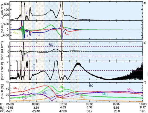
Figure 6 presents the results from the curlometer. The blue shaded areas indicate the time intervals when the ring current population is observed in C1 data. These blue areas can also be seen on Fig. 2b. The L-shell and the magnetic latitude of C1 is given in Fig. 6. As the current density is calcu-lated using the four satellites, these values are indicative and only give an average position. Frame a shows the time evo-lution of|Jav|and its components in cylindrical coordinates. We can notice first thatJav and its components go to infin-ity before entering inside the ring current (between 05:25 UT and 05:36 UT) and during the second slot region crossing (at about 06:55 UT). This strong increase is linked with a strong increase of divB(frame b, top panel) which also goes to in-finity at the same time intervals. This observation indicates a very bad accuracy ofJav estimation in this part of the orbit. Moreover,P=1 at 05:30 UT and at 06:57 UT (see Fig. 2). As a consequence, the four satellites are located in the same plane and the errors made on the estimation of some of the
Javcomponents are quite important. Some oscillations
(vio-let arrows) are observed between 05:30 UT and 05:48 UT on
Jav and on its components. These oscillations are also ob-served on divB. A more detailed study of the magnetic field data allows showing that they come from Pc5 ULF pulsa-tions, which are responsible for oscillations in the magnetic field lines. A more detail study of this phenomenon is out of the scope of the paper.
From 05:48 UT the four satellites are located in the ring current region. Javcalculated using the curlometer is equal
or higher than 100 nA m−2 between the two strong increas-ing ofJav and close to 200 nA m−2after the second strong
increasing ofJav. Focusing now on theJavcomponents,
az-imuthal, radial and parallel to the z-axis currents are observed all along the ring current region crossing. In the cylindrical coordinates, the ring current flows in the azimuthal direc-tion. It flows eastward ifJavϕ is positive and westward if
Javϕ is negative. The current in the radial and parallel to the z-axis directions indicate the existence of radial and/or field aligned currents. The average current density in the azimuthal direction obtained using the curlometer is nega-tive until 06:03 UT, indicating a westward ring current. At 06:03 UT, the azimuthal current direction changes to become eastward at L=3.59RE. This result is in agreement with
S. Grimald et al.: Study of the applicability of the curlometer technique 603
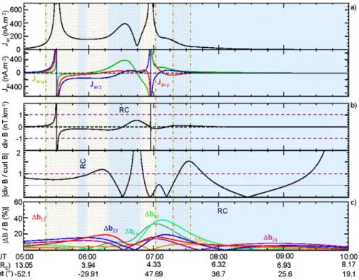
Fig. 6.Estimation of the current density along the Cluster orbit on 15 May 2009 ring current region crossing. Frame(a): time evolution of |Jav|(top panel) and its components in cylindrical coordinates (bottom panel). Frame(b): divBand|divB
cur l B|. Frame(c):1bij=
Bi−Bj/B, withiandjthe satellite number (panela). In each frame, the blue shaded areas indicate the time intervals when the ring current is observed on C1 data. The brown dashed lines are located where|divB| =1 nT km−1. The L-shell and the magnetic latitude of C1 is given in Fig. 6. As the current density is calculated using the four satellites, these values are indicative and only give an average position.
between 3RE and 4RE (Le et al., 2004; Jorgensen et al.,
2004). Then the average current density increases to reach 360 nA m−2at the perigee pass. After the second slot region crossing, the average current density in the azimuthal direc-tion is eastward and about equal to 170 nA m−2. Then, it decreases to reach zero at 09:17 UT (L=7.3RE). It never
becomes westward.
What about the accuracy of this result? In Fig. 6, the brown dotted-dashed lines indicates the time when|divB| = 0.1 nT km−1. Between two lines, in the dotted regions, |divB|>0.1 nT km−1, so divB is much greater than zero. As a consequence, the Maxwell-Thomson law (divB=0) is violated during these parts of the orbit and the average cur-rent density obtained from the curlometer may be inaccu-rate. In the other part of the orbit, divBis close to zero. As shown during the development of the method, a divBclose to zero is a necessary but not adequate condition for an accu-rate value ofJav. A better quality factor has been shown to be divB
cur l Bas it is dimensionless. Moreover, the mag-netic field has to change slowly from a satellite to another. |DivB/curlB|is presented in the second panels of frame b in Fig. 6. It is noticeable that|DivB/curlB|is very noisy dur-ing part of the orbit, which may be due to the error on the magnetic field measurement. Frame c (Fig. 6) presents the time evolution of1bij (where1bij=(BCi−BCj)/B, withi
andj the satellite number). We can notice first that the same oscillations as the ones observed on divB, onJav and on its components are seen on1bij, which confirm that they come from oscillations on the magnetic field lines. During the main part of the ring current region crossing, divB
cur l B
is above 0.5 (dotted purple line), indicating a standard de-viation higher than 50 %, and there is always a1bij higher than 25 %. As a consequence, the curlometer technique is not valid during the whole ring current crossing, even when |divB|<0.1 nT km−1.
4 Study of the accuracy of the curlometer technique along the Cluster orbit
4.1 Current density from the Tsyganenko model
In this paper, the curlometer technique has been used to cal-culate the current density between 2 and 7RE. It has been
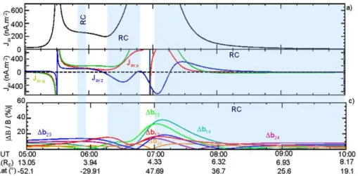
Fig. 7.Same as Fig. 6, but using a Tsyganenko model.
of the measurement errors have not been mentioned in the previous part, but it has been shown that these errors increase strongly the uncertainty ofJav(Dunlop et al., 2002; Vallat et al., 2005). Moreover, it has been shown that variations in the solar wind are responsible for injections of particles and for compression of the magnetosphere. The Dst index variations associated with increasing auroral indices is very smooth. As stated above, this observation assumes that the ring current is not (or is only very slightly) disturbed. However, changes in the ring current are responsible for distortion of the mag-netic field lines and will impact the results obtained using the curlometer technique. In order to suppress those uncer-tainties, a Tsyganenko model (Tsyganenko and Stern, 1996) has been used to calculate the magnetic field along the Clus-ter orbit and to test the curlomeClus-ter technique along this orbit. Using a model, the position of the satellites and the mag-netic field is known without errors. Moreover, the parame-ters of the model have been defined to model a quiet mag-netosphere with no injection of particles and no compres-sion of the magnetopause. As a consequence, the satellites cross a non-disturbed ring current. The results obtained us-ing the curlometer technique in such a magnetic field for the 15 May 2009 perigee pass is presented in Fig. 7, which is similar to Fig. 6. The1bij obtained using the Tsyganenko model show some differences from the ones obtained using the FGM magnetic field, but the evolutions and the magni-tudes are similar. Nevertheless, we have to notice first that they are slightly smaller as the maximum of the1bij for the FGM data is 50 % when it is 37 % for the Tsyganenko model,
and second that the oscillations observed before the entrance in the ring current region in the FGM data are not observed in the Tsyganenko magnetic field, as they come from the varia-tion of the magnetospheric activity. Looking now atJavand divB, the temporal evolution ofJav and divB is similar to the ones obtained using the FGM data. In particular, they go to infinity at the same time because of the planar tetrahedron, currents in the azimuthal, radial and parallel to the z-axis cur-rent are observed, and the azimuthal curcur-rent is first westward and then eastward. As the one obtained using the FGM data the azimuthal current is eastward after the second slot region crossing and never becomes westward. A difference can be observed in the values of the current and of the divB, which are slightly smaller due to smaller1bij.
What about the accuracy of this result? As in Fig. 6, the brown dotted-dashed lines in Fig. 7 indicates the time when |divB| =0.1 nT km−1and the dotted regions, the time when the Maxwell-Thomson law (divB=0) is violated. The dot-ted part obtained for the model and the data are about the same. Comparing now the divB
S. Grimald et al.: Study of the applicability of the curlometer technique 605
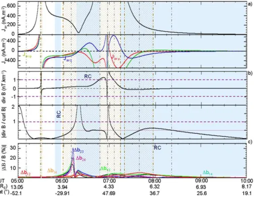
Fig. 8.Estimation of the current density and1bij along the Cluster orbit on 15 May 2009 ring current region crossing for a dipolar model. In each frame, the blue shaded areas indicate the time intervals when the ring current is observed on C1 data.
uncertainties on the results are still too important and the cur-lometer technique is not valid during the whole ring current region crossing.
4.2 Current density from the dipolar model
In Sect. 4.1, the curlometer technique has been used on a Tsy-ganenko model. The results obtained show that the low ac-curacy of the method on the 15 May 2009 doesn’t come from nonlinear gradients induced by the magnetospheric activity, nor from the uncertainties on the position of the satellites or on the magnetic field data. In the Tsyganenko model, the magnetic field is made up of an internal and an external mag-netic field. The internal magmag-netic field chosen in this study is a dipolar one. The external magnetic field comes from the magnetic field induced by the magnetospheric currents as the magnetopause current or the ring current. By defini-tion, the current calculated using the Maxwell-Ampere’s law for a dipolar magnetic field has to be equal to zero. Non-zero values would be representative of errors induced by the cur-lometer technique. Using a Cluster orbit, Vallat et al. (2005) show that this error doesn’t affect significantly the current density calculation. To do so, they used two current densi-ties obtained at a perigee located at 4RE. On 15 May 2009,
the perigee was located at about 2REand it is plausible that
the effect of the dipolar model on theJavcalculation is more important. In order to address this question, the curlometer has been used to calculateJav using a dipolar model. The obtainedJav and its components obtained are presented in Fig. 8 (frame a) as well as1bij (frame b). As in Figs. 2, 6 and 7 the blue shaded areas indicate the time intervals when the ring current population is observed in C1 data. A strong current is observed during the main part of the cross-ing. This current is in the azimuthal, radial and parallel to the z-axis direction. This result indicates a strong contribution of the dipole to the current calculation for this event, which
is, therefore, not reliable. Moreover, the1bij obtain using the dipolar model is very similar to the ones obtain using the Tsyganenko model and no clear differences are visible. As a consequence, the very bad accuracy of the method for this event may come from nonlinear gradients induced by the distance between the satellite and the quick evolution of the magnetic field close to the Earth.
4.3 Current density from the distortion of the Tsyganenko magnetic field
It has been shown in the previous section that the dipolar magnetic field induces a strong current in theJav calcula-tion. As a consequence,Jav=Jav dip+Jav RC, whereJav dip
Fig. 9. Same as Fig. 6, but using a magnetic field calculated by subtracting a dipolar magnetic field from the Tsyganenko one. The grey dotted-dashed lines indicate the times when divB
cur l B=5.
it increases to turn eastward at 06:18 UT (L=2.55RE). As
the one obtained using the FGM and the Tsyganenko mag-netic fields, it is eastward after the second slot region cross-ing and never becomes westward again.
What about the accuracy of this result? As in Fig. 6, the brown dotted-dashed lines in Fig. 9 indicates the time when |divB| =0.1 nT km−1and the dotted regions, the time when the Maxwell-Thomson law (divB=0) is violated. The dot-ted part obtained for the model and the data are about the same. Looking now on the divB
cur l B temporal
evo-lution, it is interesting to note that it is below 5 between 05:15 UT and 06:10 UT, 06:47 UT and 06:57 UT, 07:05 UT and 07:40 UT, and from 08:20 UT (grey dotted-dashed lines in Fig. 9 indicate those times). During each interval, it goes very close to zero, indicating a good accuracy of the method. Nevertheless, during part of the first and the third interval and during the whole second interval divB>0.1 nT m−2. More-over,Javincreases strongly during the second and third in-terval indicating strong errors in the curlometer results. If we consider that divB<0.1 nT m−2 indicates a good ac-curacy of the method, then, Jav may be correct between 05:15 UT (L=10.26RE) and 06:10 UT (L=3.07RE) and
from 08:20 UT (L=6.3RE). We will now study in more
de-tails the value, the current density and the orientation of the current for each time interval.
Looking first at Jav during the first interval, it goes to infinity until 05:30 UT and then decreases slowly from 400 nA m−2 to 350 nA m−2. Vallat et al. (2005)
deter-mined for the 18 March 2002 perigee pass between L= 4.2RE and 5RE and found 20 nA m−2<Jav<30 nA m−2.
On 15 May 2009, the satellites are located in a [3.07RE;
7.77RE] L-shell range between 05:30 UT and 06:10 UT and
cross the L-shell studied by Vallat et al. (2005). The av-erage current density obtained here is 10 times higher than the one they obtained. It has been shown that the error can be different from one Jav component to another and in particular, that close to perigee, it will be more impor-tant on the parallel to the z-axis component. Therefore, we will now compare the azimuthal currents obtained for the 18 March 2002 and the 15 May 2009. For each event, a con-stant azimuthal current is obtained, but it is about equal to −200 nA m−2on the 15 May 2009, when it has been found at about−20 nA m−2on 18 March 2002. As a consequence, the results obtained for the first interval on the 15 May 2009 looks to be inaccurate.
Looking now at the second time interval, Jav decreases from 50 nA m−2to 5 nA m−2as well asJ
avϕ, which appears to be a closer value to the one obtained for the 18 March 2002 event. All the same, fromL=6.3RE, the current defined in
the model is westward andJavϕ has to be negative when the one calculated using the curlometer is positive. Such results indicate that, despite low divB, divB
S. Grimald et al.: Study of the applicability of the curlometer technique 607
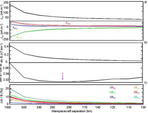
Fig. 10. Jav, its components (framea), divB(frameb), divBcur l B(frameb), and1bij (framec) versus the interspacecraft separation distance. The violet arrow is located at about 220 km separation distance. For this value, the best accuracy of the curlometer has been obtained.
5 Calculation of the current density for smaller separations
5.1 Study of the curlometer results at the perigee pass for different separations
Along the Cluster orbit, the shape of the tetrahedron changes: it is very elongated at perigee passes and flattened in the cusp crossings. To use the curlometer technique, the size of the tetrahedron has to be small enough so that the four satellites are located in the same current sheet and the magnetic field gradients are as linear as possible. At the same time, it has to also be big enough so as the magnetic field gradients are de-tectable from one satellite to another. For the 15 May 2009 ring current density calculations, the four satellites are lo-cated in the same current sheet, but the1B/B is quite high for the whole ring current region crossing. This result in-dicates that the distance between the satellites is too large to suppose that the magnetic field measured on board each satellite is very close to each other (linear gradient assump-tion). In the perspective of future missions, this addresses the question of whether the curlometer technique could be used for a smaller spacecraft separation. To answer this question, the first point is to determine for which interspacecraft sep-arations accurate values of Jav are obtained. To do so, a given point of the 15 May 2009 orbit has been chosen to test the accuracy of the curlometer for different separations. As
the method is inaccurate because of the rapid spatial evolu-tion of the magnetic field, the perigee pass, where the mag-netic field and its variations are the most important, has been chosen. Then, the curlometer has been used in the Tsyga-nenko magnetic field used in Sect. 4.2 for simulated tetra-hedrons obtained by reducing its size by a factor between 1 and 10. Figure 10 presentsJav, its components (frame a), divB(frame b), divB
cur l B(frame b), and1bij(frame c) versus the interspacecraft separation distance. Focusing on the divB
cur l Bevolution, it is noticeable that it decreases until 220 km separation (violet arrow in Fig. 10), and then increases, showing that it exists a separation leading to the best accuracy ofJav. Unfortunately, divB
cur l B≈2.01 at its minimum, indicating not a good accuracy of the method at the perigee pass even for this separation.
5.2 Current density for a 220 km separation
It has been shown that 220 km separation gives the best ac-curacy of the curlometer for a perigee pass located at about 2RE, but that the error is quite important at this position. The
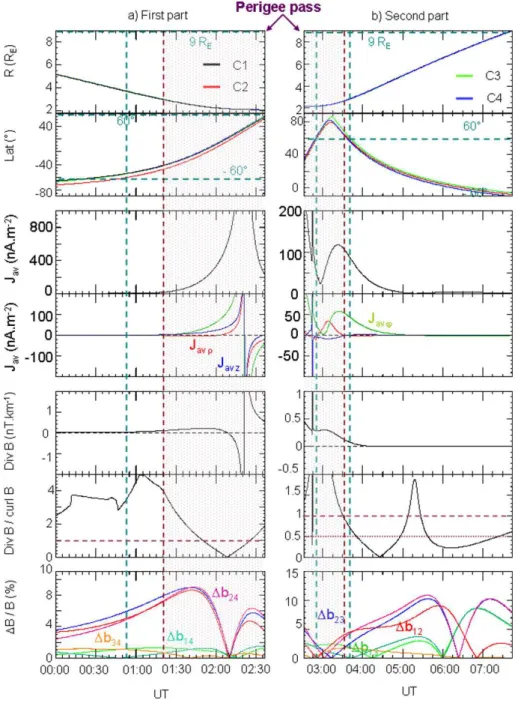
Fig. 11.Study of the accuracy of the curlometer technique for the Tsyganenko magnetic field calculated along a modelled orbit with 200 km separation.
(first panel) and the magnetic latitude (second panel) of the four satellites during the ring current region crossing. The perigee is located at 2RE and is crossed at 02:35 UT. As
it was necessary to use different scales before and after the perigee pass, the figure has been divided in two columns: be-fore the perigee pass in the left part of the figure (annotated “a”) and after the perigee pass in the right part of the figure (annotated “b”). It is clear from this plot that the satellites are very close to each other. As the ring current is typically ob-served in a (2RE; 9RE) geocentric distance range and±60◦
magnetic latitude (Vallat et al., 2005), horizontal blue dashed
lines (first frames of Fig. 11a and b) have been located at 9RE
(first panels) and at±60◦magnetic latitude (second panels). The vertical blue dashed lines indicate the boundaries of the ring current: the satellites are located inside the ring cur-rent in a [00:54 UT; 02:40 UT] and in a [03:40 UT; 07:15 UT] time range. The magnetic field along the orbit has been cal-culated using a Tsyganenko model (Tsyganenko and Stern, 1996) and then used to calculate the current density from the curlometer. The third and the fourth frames of Fig. 11 present the results obtained from the calculations (Jav, its
S. Grimald et al.: Study of the applicability of the curlometer technique 609
The last frame presents the time evolution of 1bij which is never higher than 12 %. As in Figs. 6, 7 and 9, the brown dashed lines are located where|divB| =0.1 nT km−1
and the brown dotted areas indicate when divB >0.1. In panel (a), the satellites are located in the ring current region and|divB|<0.1 between 00:54 UT and 01:21 UT. Unfor-tunately, during this time range, divB
cur l B>3.6. As a consequence, the accuracy of the curlometer technique is small for this part of the orbit. Focusing now on the sec-ond part of the orbit (figure b), the satellites are located in the ring current region and|divB|<0.1 from 03:40 UT. divB
cur l B<0.5 between 04:47 UT and 05:00 UT, and between 05:40 UT and 07:15 UT. As a consequence, the cur-lometer parameters indicate that the calculation may be ac-curate for such an orbit in an [3RE; 5RE] and [6RE; 8.3RE]
L-shell range with a 220 km separation.
6 Discussion and conclusion
In this paper, the curlometer technique has been used to cal-culate the current density much deeper inside the inner mag-netosphere than ever before. In the first instance, the calcu-lation was performed for a medium inter-spacecraft separa-tion of the 4 Cluster satellites (1000 km) using the magnetic field time series measured by the FGM instruments during the 15 May 2009 ring current region crossing and using also three modelled magnetic field time series calculated along the same orbit (from an empirical model, a dipolar model and by subtracting the dipolar from the empirical magnetic field values). The results can be summarized as follows:
1. The Maxwell-Thomson law (divB=0) is violated for each of the four magnetic field inputs, and divB
cur l B and 1B/B are quite high for at least part of each time series. These results come from the rapid change of the magnetic field magnitude associated with the increased elongation of the tetrahedron at the perigee pass.
2. A non-zero current density has been obtained for the dipolar model showing the inadequacy of the method for this orbital configuration.
3. Regarding the last magnetic field model (BTsyganenko− Bdipole), divB, divB
cur l B and 1B/B evolutions seem to indicate a good accuracy of the method when the azimuthal current density is higher than the past results.
This study shows that the current density cannot be cal-culated using the curlometer technique for Cluster orbits with low altitude perigee passes, where the inter-spacecraft separation becomes too large. Moreover, we find that divB, divBcur l B and 1B/B characteristics are not enough to evaluate the accuracy of the method: divB≈0,
divB
cur l B≪1 and1B/B≪1 are necessary but not suf-ficient conditions. The next step was to find a new condition that had to be sufficient to test the accuracy of the curlometer. Furthermore, it was shown that the error could vary from a current density to another. In particular, as the tetrahedron becomes more and more elongated when travelling to the perigee, the error on the z-component is higher than for the x- and the y-components. Thus, it was found useful to de-fine a test of the accuracy for each component of the current density calculated using the curlometer.
As a second step, the curlometer has been used at the perigee pass for different inter-spacecraft separations. This study shows that a separation that leads to the best accuracy of the method could be defined. It also shows that the cur-rent density cannot be calculated using the curlometer tech-nique for perigee passes located as low as 2RE.
Neverthe-less, the calculation may be accurate within [3RE; 5RE] and
[6RE; 8.3RE] L-shell ranges, which are deeper inside the
inner magnetosphere than what has been reported in the past. Other methods are under development, which may work along such an orbit. Moreover, the MMS (Multi scale Mag-netospheric Satellites) mission is composed of four satellites, which will have a separation of 10 to 200 km and a perigee located at 1.2REgeocentric distance. Those satellites, to be
launched in 2014, will have a separation distance very close to the one leading to the best accuracy of the method. It may bring new information about the current density in the inner magnetosphere and the parameters we have to use to test the accuracy of the curlometer.
Acknowledgements. S.G. acknowledges financial support from the Centre National d’Etudes Spatiales (CNES). We would like to thank the WEC, JSOC and ESOC teams for continuous support of Clus-ter operations. The authors thank the FGM and the CIS teams for preparing the data used in this paper, and the CAA for mak-ing the Cluster data available to the community. We also acknowl-edge the WDC for providing the magnetic indices. Data analysis was done with the QSAS science analysis system provided by the United Kingdom Cluster Science Centre (Imperial College London and Queen Mary, University of London) supported by STFC and the CL analysis software developed at IRAP.
Guest Editor M. Taylor thanks two anonymous referees for their help in evaluating this paper.
References
Alfv´en, H.: Some properties of magnetospheric neutral surfaces, J. Geophys. Res., 73, 4379–4381, 1968.
Balogh, A., Dunlop, M. W., Cowley, S. W. H., Soothwood, D. J., Thomlinson, J. G., Glassmeier, K. H., Musmann, G., Luhr, H., Buchert, S., Acuna, M. H., Fairfield, D. H., Slavin, J. A., Riedler, W., Schwingenschuh, K., and Kivelson, M. G.: The Cluster mag-netic field investigation, Space Sci. Rev., 79, 65–91, 1997. Balogh, A., Carr, C. M., Acu˜na, M. H., Dunlop, M. W., Beek, T.
J., Brown, P., Fornacon, H., Georgescu, E., Glassmeier, K.-H., Harris, J., Musmann, G., Oddy, T., and Schwingenschuh, K.: The Cluster Magnetic Field Investigation: overview of in-flight performance and initial results, Ann. Geophys., 19, 1207–1217, doi:10.5194/angeo-19-1207-2001, 2001.
Buzulukova, N. Y., Galperin, Y. I., Kovrazhkin, R. A., Glazunov, A. L., Vladimirova, G. A., Stenuit, H., Sauvaud, J. A., and Delcourt, D. C.: Two types of ion spectral gaps in the quiet inner magneto-sphere: Interball-2 observations and modeling, Ann. Geophys., 20, 349–364, doi:10.5194/angeo-20-349-2002, 2002.
Chanteur, C.: Spatial interpolation for four spacecraft: theory, in Analysis Methods for Multi-Spacecraft data, ISSI Sci. Rep. SR-001, 323–448, 1998.
Chanteur, C. and Mottez, F.: Geometricl tools for Cluster data analysis, in: Proc. International Conf, “Spatio-temporal Anal-ysis plasma turbulence (START), Aussois, 31 January–5 Febru-ary 1993, ESA WPP-047, pp. 341–344, European Space Agency, Paris, France, 1993.
Chen, M. W., Lui, S., Schulz, M., Roeder, J. L., and Lyons, L. R.: Magnetically self-consistent ring current simulations dur-ing the 19 October 1998 storm, J. Geophys. Res., 111, A11S15, doi:10.1029/2006JA011620, 2006.
Daglis, I. A., Sarris, E. T., and Wilken, B.: AMPTS/CCE CHEM observations of the ion population at geosynchronous altitude, Ann. Geophys., 11, 685–696, 1993,
http://www.ann-geophys.net/11/685/1993/.
Dunlop, W. M., Southwood, D. J., Glassmeier, K.-H., and Neubauer, F. M.: Analysis of multipoint magnetometer data, Adv. Space Res., 8, 9–10, 1988.
Daglis, I. A., Thorne, R. M., Baumjohann, W., and Orsini, S.: The terrestrial ring current: origin, formation, and decay, Rev. of Geophys., 37, 407–438, 1999.
Dandouras, I., Cao, J., and Vallat, C.: Energetic ion dynamics of the inner magnetosphere revealed in coordinated Cluster-Double Star observations, J. Geophys. Res., 114, A01S90, doi:10.1029/2007JA012757, 2009.
Dunlop, M. W. and Balogh, A.: On the analysis and the interpreta-tion of the four spacecraft magnetic field measurements in term of small scale plasma processes, in Spatio-Temporal Analysis for Resolving Plasma Turbulence (START), Eur. Space Agency, WPP, ESA WPP-047, p. 223, 1993.
Dunlop, M. W., Balogh, A., Glassmeier, K.-H., and Robert, P.: Four-point Cluster application of magnetic field analysis tools: the curlometer, J. Geophys. Res., 107, 1384–1398, 2002. Ejiri, M.: Trajectory traces of charged particles in the
magnetosphere, J. Geophys. Res., 83, 4798–4810, doi:10.1029/JA083iA10p04798, 1978.
Escoubet, C. P., Fehringer, M., and Goldstein, M.: Introduc-tion “The Cluster mission”, Ann. Geophys., 19, 1197–1200, doi:10.5194/angeo-19-1197-2001, 2001.
Ganushkina, N. Yu., Dandouras, I., Shprits, Y. Y., and Cao, J.: Locations of Boundaries of Outer and Inner Radiation Belts as Observed by Cluster and Double Star, J. Geophys. Res., 116, A09234, doi:10.1029/2010JA016376, 2011.
Gloeckler, G. B., Wilkinen, W., St¨udemann, F., Ipavich, F. M., Hov-estadt, D., Hamilton, D. C., and Kremser, G.: First composi-tion measurement of the bulk of the storm-time ring current (1 to 300 keV/e) AMPTE/CCE, Geophys. Res. Lett., 12, 325–328, 1985.
Hamilton, D. C., Gloeckler, G., Ipavitch, F. M., St¨udemann, W., Wilken, B., and Kremser, G.: Ring current development during the great geomagnetic storm of February 1986, J. Geophys. Res., 93, 14343–14355, 1988.
Jordanova, V. K.: New Insights on Geomagnetic Storms from Model Simulations Using Multi-Spacecraft Data, Space Sci. Rev., 107, 157–165, doi:10.1023/A:1025575807139, 2003. Jordanova, V. K., Miyoshi, Y. S., Zaharia, S., Thomsen, M. F.,
Reeves, G. D., Evans, D. S., Mouikis, C. G., and Fennell, J. F.: Kinetic simulations of ring current evolution during the Geospace Environment Modeling challenge events, J. Geophys. Res., 111, A11S10, doi:10.1029/2006JA011644, 2006.
Jorgensen, A. M., Spence, H. E., Hughes, W. J., and Singer, H. J.: A statistical study of the global structure of the ring current, J. Geophys. Res., 109, A12204, doi:10.1029/2003JA010090, 2004. Krimigis, S. M., Gloeckler, G., McEntire, R. W., Potemra, T. A., Scarf, F. L., and Shelley, E. G.: Magnetic storm of September 4, 1984: A synthesis of ring current spectra and energy densities measured with AMPTE/CCE, Geophys. Res. Lett., 12, 329–332, 1985.
Le, G., Russell, C. T., and Takahashi, K.: Morphology of the ring current derived from magnetic field observations, Ann. Geo-phys., 22, 1267–1295, doi:10.5194/angeo-22-1267-2004, 2004. Lui, A. T. Y. and Hamilton, D. C.: Radial profiles of quiet time
magnetospheric parameters, J. Geophys. Res., 97, 19325–19332, 1992.
Lui, A. T. Y., Mc Entire, R. W., and Krimigis, S. M.: Evolution of the ring current during two geomagnetic storm, J. Geophys. Res., 92, 7459–7470, 1987.
McIlwain, C.: Plasmaconvection in the vicinity of the geosyn-chronous orbit, in Earth’s Magnetospheric Processes, McCor-mac, B., p. 268, D. Reidel Pub. Comp., 1972.
S. Grimald et al.: Study of the applicability of the curlometer technique 611
magnetosphere with the identical Cluster ion spectrometry (CIS) experiment, Ann. Geophys., 19, 1303–1354, doi:10.5194/angeo-19-1303-2001, 2001.
Robert, P. and Roux, A.: Dependance of the shape of the tetrahedron on the accuracy of the estimate of the current density, in Spatio-temporal Analysis for Resolving Plasma Turbulence (START), Eur. Space Agency, WPP, ESA WPP-047, 289–193, 1993. Robert, P., Dunlop, M. W., Roux, A., and Chanteur, G.: Accuracy
of current density determination, in Analysis Methods for Multi-Spacecraft data, ISSI Sci. Rep. SR-001, 395–418, 1998a. Robert, P., Roux, A., Harvey, C. C., Dunlop, M. W., Daly, P. W., and
Glassmeier, K.-H.: Tetrahedron geometric factors, in: Analysis Methods for Multi-Spacecraft data, ISSI Sci. Rep. SR-001, 323– 448, 1998b.
Roelof, E. C., C:son Brandt, P., and Mitchell, D. G.: Derivation of currents and diamagnetic effects from global plasma pressure distributions obtained by IMAGE/HENA, Adv. Space Res., 33, 747–751, 2004.
Sauvaud, J.-A., Barthe, H., Aoustin, C., Thocaven, J. J., Penou, E., Rouzaud, J., Kovrazhkin, R. A., Afanasiev, K. G., and Ivanchenkova, I. Yu.: Measurement of the suprathermal plasma by ION spectrometric complex on the Interball-2 satellite (Auro-ral probe), Cosmic Research, 36, 59–68, 1998a.
Sauvaud, J. A., Barthe, H., Aoustin, C., Thocaven, J. J., Rouzaud, J., Penou, E., Popescu, D., Kovrazhkin, R. A., and Afanasiev, K. G.: The ion experiment onboard the Interball-Aurora satel-lite; initial results on velocity-dispersed structures in the cleft and inside the auroral oval, Ann. Geophys., 16, 1056–1069, doi:10.1007/s00585-998-1056-z, 1998b.
Singer, S. F.: A new model of magnetic storms and aurorae, Eos Trans. AGU, 38, 175–190, 1957.
Shirai, H., Maezawa, K., Fujimoto, M., Mukai, T., Saito, Y., and Kaya, N.: Monoenergetic ion drop-off in the in-ner magnetosphere, J. Geophys. Res., 102, 19873–19881, doi:10.1029/97JA01150, 1997.
Smith, P. H. and Hoffman, R. A.: Ring current particle distribu-tions during the magnetic storms of December 16–19, 1971, J. Geophys. Res., 78, 4731–4737, 1973.
Stern, D. P.: The motion of a proton in the equatorial magneto-sphere, J. Geophys. Res., 80, 595–599, 1975.
Tsyganenko, N. A. and Stern, D. P.: Modeling the global magnetic field of the large-scale Birkeland current systems, J. Geophys. Res., 101, 27187–27198, 1996.
Vallat, C., Dandouras, I., Dunlop, M., Balogh, A., Lucek, E., Parks, G. K., Wilber, M., Roelof, E. C., Chanteur, G., and R`eme, H.: First current density measurements in the ring current re-gion using simultaneous multi-spacecraft CLUSTER-FGM data, Ann. Geophys., 23, 1849–1865, doi:10.5194/angeo-23-1849-2005, 2005.
Vallat, C., Ganushkina, N., Dandouras, I., Escoubet, C. P., Taylor, M. G. G. T., Laakso, H., Masson, A., Sauvaud, J.-A., R`eme, H., and Daly, P.: Ion multi-nose structures observed by Clus-ter in the inner Magnetosphere, Ann. Geophys., 25, 171–190, doi:10.5194/angeo-25-171-2007, 2007.
Volland, H.: A semi empirical model of large-scale mag-netospheric electric fields, J. Geophys. Res., 78, 171, doi:10.1029/JA078i001p00171, 1973.