Flavio H. Fernández Morales
[email protected] Univ. Pedagógica y Tecnológica de Colombia Facultad Seccional Duitama Duitama, Boyacá. Colombia
Sergio Leseduarte Cuevas
[email protected] Universitat de Barcelona Departament d’Electrònica 08028, Barcelona, Spain
Josep Samitier i Martí
[email protected] Universitat de Barcelona Departament d’Electrònica Barcelona, Spain
Numerical Analysis of Thermal and
Electrohydrodynamic Effects in
Travelling-Wave Dielectrophoretic
Devices
Travelling-wave dielectrophoretic phenomena involving cell detection and manipulation are very interesting for biomedical and biotechnological applications. However, electrohydrodynamic phenomena may interfere with the action of dielectrophoresis. The main goal of our study is to calculate the interplay of these effects. In so doing, we have been able to go beyond the order-of-magnitude estimations, which were available in the literature. In this framework we have taken into account the effects of using square signals, which calls for a calculation of the combined polarisability effects due to the superposition of different frequencies. Thermal gradients are also a triggering agent of electrohydrodynamic effects. We have undertaken the pertinent thermal simulations with a concern for the influence of different boundary conditions. The dynamics of the thermal fields were also assessed in order to estimate the characteristic times of electrohydrodynamic phenomena. All these results have been used in a study of the fluid flow pattern motion at different frequencies and its influence on the particle behaviour.
Keywords: computer modelling, Micromanipulators, electrohydrodynamics, dielectrophoresis
Introduction
1
It has been known for a long time that an electric field in a suspension containing a polarisable material will induce a charge distribution on the particle's surface, which will accordingly behave as an effective dipole.
When a non-uniform electric field is applied, particles, behaving as dipoles, experience a net force, which carries them towards or away from the field maximum, depending on the relation between the electrical properties (i.e. permittivity and conductivity) of particles and medium. This force causes the particle motion. This phenomenon of neutral-matter motion arising from its interaction with a non-uniform electric field was called dielectrophoresis (DEP) by Pohl (1951). This simple definition embeds three phenomena: common DEP (c-DEP), electrorotation (ROT) and travelling wave dielectrophoresis (TWD) which differ in the characteristics of the electric field: c-DEP is originated by electric fields inhomogeneous in amplitude, ROT is generated by rotary electric fields inhomogeneous in phase and TWD is produced by travelling wave of electric fields with inhomogeneities in both magnitude and phase.
Furthermore, the force exerted on a particle varies with the frequency of the applied signal and making good use of this, DEP has been employed to characterise latex microparticles (Green and Morgan, 1999), and biological organisms (Müller et al., 2003), and to fabricate microdevices addressed to handling and manipulating cells and macromolecules (Rosenthel and Voldman, 2005), to perform linear motion and separation of cells and latex microbeads (Talary et al., 1996; Masuda et al., 1987), microparticle conveyors forming part of laboratory-on-a-chip devices (Pethig et al., 1998) and devices to concentrate and assay the viability of micro-organisms (Goater et al., 1997).
The electric conductivity of slightly conducting liquids often depends on temperature. Hence, if a thermal gradient is imposed inside the liquid, such as that arising from the Joule heating effect, it gives rise to a gradient in the liquid electrical conductivity and permittivity. Besides that, if a travelling electric field is imposed in the structure, it originates the bulk interaction of fluid with the travelling potential wave through the mechanism of a thermally
Paper accepted August, 2007. Technical Editor: Paulo E. Miyagi.
induced gradient in electrical conductivity and permittivity that produces fluid motion (Melcher and Firebaugh, 1967). This effect has been used as a mechanism of actuation to pump fluids in microchips (Müller et al., 1993).
A review of the order-of-magnitude for the force on submicrometer particles in non-uniform alternating current (AC) electrical fields was carried out by Ramos and co-workers (1998). This theoretical study compares the relationship between forces acting in common-dielectrophoresis-based-devices (c-DEP devices), such as dielectrophoretic forces, Brownian motion and diffusion as well as electrohydrodynamic (EHD) effects triggered by the Joule heat generation effect caused by the applied potential. It was mentioned that EHD forces can affect the stable trapping of particles smaller than 1 µm, and, depending on the experimental conditions, the fluid velocity motion will govern the particle behaviour instead of the desired c-DEP forces.
Despite the huge range of applications up to now the theoretical and numerical studies of DEP have concentrated on the electric field and dielectrophoretic force distributions (Wang et al., 1994; Hughes
et al., 1996). On the other hand, the lack of calculations taking into
account the influence of other related phenomena such as EHD is noticeable. Of course, to design much more reliable and controllable devices, for instance based on TWD, the influence of EHD phenomena has to be considered, especially when working with media of high conductivities and high-applied voltages.
Our goal in this paper is the development of a general simulation methodology to study and calculate the particle dynamics, when subjected to DEP forces, in the case of TWD systems. The EHD effects involved in it have been taken into account. The employed methodology can be easily adapted to other geometries and DEP effects such as electrorotation.
The second section is devoted to the calculation of the time-varying electric field for a common TWD application with square-bipolar signals and to the correction of the Clausius-Mosotti factor for this case. The calculation of the electric field is required for the thermal analysis, because it determines the loads. The correction to the Clausius-Mosotti factor is a useful result for the proper evaluation of DEP forces on a particle, in particular if it is necessary to compare DEP forces and drag forces induced by EHD effects.
Also, the influence of the chip substrate and the ensuing thermal boundary conditions (BCs) is studied by means of a two-dimensional (2-D) axisymmetrical model solved through the commercial program Ansys (Swanson Analysis Systems Inc.), which uses the Finite Element Method (FEM) for the solving of physical problems and which has been used for all FEM analysis in this work. The thermal analysis is presented in section three. The load for the thermal problem is the Joule effect induced in a conductive medium by the presence of the electric field, previously calculated. The results of this section are interesting because thermal gradients may be triggering agents of EHD phenomena as explained by Ramos and co-workers (1998), and their dynamics may help understand the time required for EHD phenomena to be observable. The results of the thermal FEM analysis are also required for the calculations of section fourth.
The fluid motion pattern as a consequence of EHD (electrostrictive and coulombic) forces is analysed in section “fluid model simulation”. Actually, only the lowest-order correction in terms of the applied electric signal to the unperturbed, static fluid is retained in our calculation, for which we have followed the analysis of Ramos et al., (1998). Here we use the results of sections “Electrical Modelling” and “Thermal Modelling” of that work. For this lowest-order correction, the thermal dependence of permittivity and conductivity of the medium has to be taken into account, but not that of viscosity, which would be relevant for higher-order corrections. It is apposite to note that our flow model, including fluid motion equations and inputs thereof (i.e. electric and temperature fields), takes only the fluid into account and not the presence of any particles. See the work of O’Brien (1979) for the impact of interacting particles on the transport properties (thermal conductivity and viscosity) of a suspension. Therefore, any discussion concerning the influence of the fluid flow solution as derived in this work on the motion of the suspended particles implicitly assumes a very low particle concentration and excludes situations when this condition breaks down.
Lastly, we devote section five to summary of the conclusions and a discussion of the possible interplay of DEP and EHD effects in the dynamics of suspended particles in the presence of electric fields.
Electrical Modelling
DEP Analysis Background
It is well known that if an AC electric field expressed by Eq. (1)
) ( exp )
(t E0 jω t
E = (1)
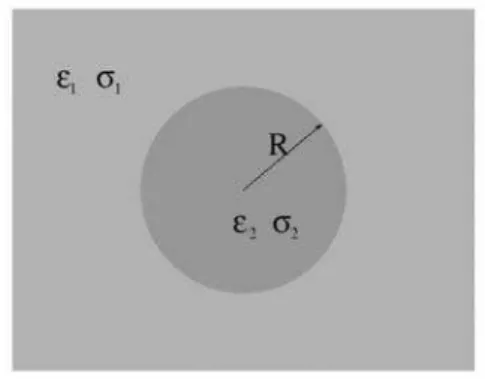
is applied to a liquid suspension which contains electrically neutral matter as depicted in Fig. 1, it will induce the appearance of an electric charge distribution onto the particle surface.
Figure 1. Spherical particle of radius R and complex dielectric permittivity
2
ε
~ given by
ω
j
σ ε
ε 2
2 2= +
~ , submersed in a liquid solution of complex
dielectric permittivity ε~1 given by
jω 1 σ 1 ε 1 ε = +
~
. εεεε1 , σσ1σσ , εεεε2 and σσ2σσ are the
permittivity and electrical conductivity of medium and particle, respectively. ωωωω is the angular frequency of the applied field.
When the particle size is small enough compared with the characteristic length of variation of the electric field, the electric charge distribution can be treated as a dipole. Taking advantage of it, the particle external potential φext can be written as:
3 1
4 1
r
eff ext
r p r
E⋅ + ⋅ ⋅
− =
ε π
φ (2)
where peff is the effective induced dipolar moment, which for a
spherical particle of radius R is given by:
E
p 3
1
4 K R
eff = π ε (3)
where K is the well-known Clausius-Mosotti factor, which represents the particle polarisability with respect to its surrounding medium and can be expressed as:
1 2
1 2
~
2
~
~
~
K
ε
ε
ε
ε
⋅
+
−
=
(4)The frequency dependence of this expression has been exploited for the characterisation and control of artificial and natural materials (Fuhr and Shirley, 1998).
When the applied electric field has spatial inhomogeneities, its interaction with the induced dipole moment gives rise to a net force, the dielectrophoretic force (FDEP), which leads the particle towards
(so called positive DEP, p-DEP)) or away from (also called negative DEP, n-DEP)) regions where the electric field strength is maximum. If the dipolar approximation is acceptable, FDEP can be expressed as:
(
p)
EFDEP = eff ⋅∇ . (5)
Moreover, if the applied field rotates, it will induce a rotational torque on the particle, which can be co- or anti-field-oriented depending on the polarity of the Clausius-Mosotti factor. This rotary torque T is given by:
E p
Dielectrophoretic Force CalculatedbBy Means of the Fourier Decomposition
In a broader sense, any periodic applied electric field can be represented by its equivalent Fourier series expansion as:
(
j kt)
e E
k k i
i exp ω
) ( ⋅
=
∑
(7)where the subscript i represents the spatial components in the Cartesian coordinate frame, k is the number of the harmonic
frequency component and ei(k) denotes the complex Fourier
coefficients, which can be written as:
(
( ))
) ( )
(k ik exp ik
i
j e
e = ⋅ − ϕ (8)
described in terms of magnitude and phase, respectively.
Employing the general electric field representation expressed by Eq. (7), the time-averaged dielectrophoretic force exerted on a spherical particle may be calculated, leading to:
(
)
(
)
∑
∑
∑
∑
∂ ⋅
−
⋅
∂ =
k
k i w
i k
i k i
k i
k i k i w w
e e R
e e R
F
) ( ) ( * ) ( (k) 1 3
) ( * ) ( (k)
1 3
K Im 4
K Re 2
ϕ ε
π ε π
(9)
where the subscript w indicates the Cartesian component of the force. The derivation of this result goes as follows: first, insert Eq. (8) into Eq. (7); then employ this result in order to have a similar Fourier expansion for the effective dipolar moment using Eq. (3); now you may combine these expansion for the dipolar moment and the electric field to derive an expression for the DEP force at any time (Eq. (5)), the time average over one period being Eq. (9).
Two terms can be clearly identified on the right-hand side of Eq. (9). The first one is governed by the real part of the Clausius-Mosotti factor. If Re(K)>0 the particle is attracted towards regions of high-strength electric fields (p-DEP) and vice versa, i.e. if
Re(K)<0 the particle will be repelled away from those intense field
regions (n-DEP). This term is usually identified as the common dielectrophoretic force, whose magnitude also varies like the second power of the applied signal.
The second term is ruled by the imaginary part of the polarisability function and controls both rotary and travelling phenomena depending of the sign of Im(K) given by:
(
σ
2+2σ
1)(
ε
2−ε
1) (
−ε
2+2ε
1)(
σ
2−σ
1)
(10)If Im(K) is positive, particles will rotate (or translate) in a sense
that opposes that of the rotating fields and vice versa. This term also depends on the spatial phase inhomogeneities of the travelling applied field.
Particle Dynamics
The movement equation of a particle suspended in a liquid and subjected to a dielectrophoretic force can be expressed as:
(
fluid)
mb DEPR r−v + g+ F
−
= 6πη &
0 (11)
where
r
is the particle position vector. If one may calculate the DEP force, which calls for the calculation of the electric field, and the velocity flow field in the fluid, Eq. (11) makes possible the integration of the particle trajectory. In this work we explain in detail how to realise these calculations.On the right-hand side of Eq. (11) three terms are clearly identified. The first one is the Stokes drag formula for a sphere moving through a liquid with dynamic viscosity
η
. In the derivation of the Stokes formula one assumes very low Reynolds numbers (much lower than 1), which is a condition satisfied by typical dielectrophoretic applications as we shall see in section ”Analitical estimation of the DEP force”, where we estimate the magnitude of the dielectrophoretic force. The second one is the buoyancy force, which depends ong
, the acceleration due to the action of gravity, and the buoyant mass which can be expressed by:(
2 1)
3
3 4
ρ ρ π
−
= R
mb (12)
where ρ1 and ρ2 are the mass densities of fluid and particle,
respectively.
The third term denotes the previously defined dielectrophoretic force. It has to be highlighted that depending on the fluid velocity, the viscous drag force can dominate the particle behaviour instead of the desired FDEP.
If no FDEP is applied, the terminal particle velocity in the
ensuing 'free fall' situation is
R g m
v b
term= 6πη . For instance, in the
case of latex microspheres, usually employed as test particles in DEP devices, with a density of 1.05 gr cm-3 and radius of 3.4 µm
submersed in water this terminal velocity amounts to 1.4 mm s-1. The left-hand side of Eq. (11) denotes the absence of an inertial term, which is only relevant at extremely short time scales given by
η ρR2
, which using the data above yields an order of magnitude of
a few tenths of microseconds. When we solve the electric field and the fluid equations of motion, we may check that within this time scale, neither dielectrophoretic nor fluid drag forces on a particle significantly change. We implicitly assume no interactions between particles, which is true in the limit of vanishing particle volumetric fraction. Brownian motion is also ignored. Last but not least, Eq. (11) neglects lift forces as a result of the very low Reynolds numbers and no rotation model.
We have to check that particle velocities induced by buoyancy and dielectrophoretic forces are consistent with the assumption of very low Reynolds numbers. In the case of buoyancy forces (free fall), and if we use the same figures as in the previous paragraph, we get Reynolds numbers around 10-5. As for the velocity induced by dielectrophoretic forces, one may check the self-consistency of Eq. (11) with the numerical results obtained with our analysis in the sequel. The bottom line is that even forces resulting in drag velocities which are some orders of magnitude greater than the free-fall velocity for our application lead to Reynolds numbers much lower than 1.
General Field-Modelling Procedure by FEM
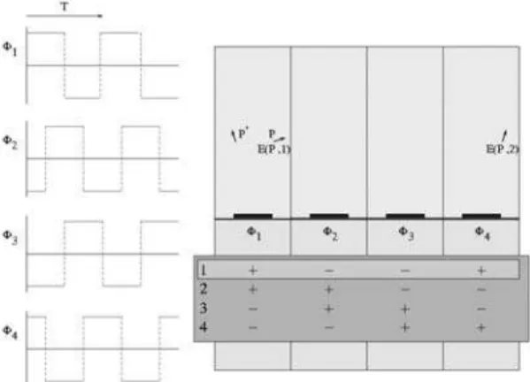
The first part of this study consists of the correct calculation of the electric field generated by four bipolar signals phased 90° from each other, which are periodically repeated every four electrodes in order to generate the travelling electric field signal.
In principle, four consecutive electrodes would have to be included in the model to obtain the whole electric field distribution. However, taking advantage of periodicity, a unique electrostatic simulation of only one electrode domain suffices to extract the complete information from the electric field at any time, as illustrated in Fig. 2(a). Looking at the field profile of a generic point
respectively. Besides that, and because of the symmetries of the problem, the electric field at point P in the second quarter of a period will be equal to the value at P', obtained from P by spatial symmetry within the same electrode domain, in the first quarter of a period but inverting its X component.
Figure 2(a). This sketch shows four consecutive electrodes driven by four bipolar signals, φφφφ1 to φφφφ4. The four possible temporal states are also depicted below the electrodes. P denotes an arbitrary point that has a field value of E(P,1) in the first quarter of a period, while P' represents the related symmetric point in the same electrode domain.
Figure 2(b). Electric field profile generated by the four voltage pattern shown in figure 2(a). The signal symmetries can be clearly seen.
It may be concluded that the four quarters of a whole electric field period can be assessed by modelling one electrode domain and performing one single electrostatic simulation. We may for instance consider boundary conditions for the leftmost domain in Fig. 2(a) in the first quarter of a period. These boundary conditions are described in Eq. (13) and Fig. 3.
(
)
(
)
(
,)
(
,)
00 ,
,
0 0
= ∂
∂ = ∂
∂
= =
= =
= =
H y x
L x y
y x y y
x x
y x y
x
φ φ
φ φ
(13)
The model employed for the calculation of the electric field assumes a plane 2-D model. However, we shall use in the following chapters the results from this calculation as input for the calculation of thermal gradients and the fluid flow using an axisymmetric model of a dielectrophoretic device, whose geometry is discussed in section “Thermal modelling”. This is a source of error, which may be effectively reduced by a wise choice of the geometric location of the electrodes in the axisymmetric thermal and fluid models, as will be explained in the next section.
Figure 3. Single electrode domain with the related BCs. The lower, thinner rectangle at the bottom is SiO2. The black one on top of it is the electrode.
The rest of the domain is occupied by fluid. L stands for the width of an electrode domain.
The DEP Electrical Model Revisited
When a non-sinusoidal signal is employed, the polarisability function has to be recalculated in order to include the effects of the high-frequency harmonic terms of the signal.
Taking into account the electric field approach described above, the dielectrophoretic force can be rewritten as:
( )
(
(
)
)
( )
×∑(
∂ − ∂)
− + × ∂ =m
m w m m w m
w w
E E E E R
R F
) 1 ( ) 2 ( ) 2 ( ) 1 ( 1
3
) 2 ( 2 ) 1 ( 2 1
3
5 . 0 ' K Im 4
5 . 0 ' K Re 2
ε π
ε
π E E
(14)
where, E(1) denotes the electric field in the first quarter of a period
and E(2) represents the electric field in the second quarter of a
period.
The whole expression for the Clausius-Mosotti factor must be modified to suit the square-signal case outlined in the last subsection. This quantity can be obtained after some straightforward but tedious calculation (see the appendix for an expression of K' and for details of its derivation and for that of Eq. (14)).
As shown in Fig. 4, the modified Clausius-Mosotti factor is somewhat rounder than the normal one. The qualitative dependence on frequency is quite similar for both factors, but it is important to point out that for some frequency ranges their real part may have large relative differences, which may have a dramatic impact on the particle motion, as explained in the following subsection, which should make it clear that the ratio of the real and imaginary parts may convey insight into the final particle velocity in TWD applications.
-1,60E-01 -1,40E-01 -1,20E-01 -1,00E-01 -8,00E-02 -6,00E-02 -4,00E-02 -2,00E-02 0,00E+00
1,00E+02 1,00E+03 1,00E+04 1,00E+05 1,00E+06 1,00E+07 1,00E+08 Freq. (Hz)
K
, K
'
(d
im
en
s
io
n
le
ss)
Re(K') Im(K') Re(K) Im(K)
Figure 4. Real and imaginary parts of the Clausius-Mosotti factor showing the differences between the 'pure' and modified Clausius-Mosotti factor (K for sinusoidal and K’ for square signals). This example is based on following material properties for medium and particles: σσσσ1= σσσσ2= 0.01 S m-1,
It is also important to know the real value and shapes of Clausius-Mosotti factor, because it is the most influential parameter in the behaviour of the dielectrophoretic force. Slight differences in this factor can move the crossover frequency bringing about big changes in the particle polarisability such as going from p-DEP to n-DEP, or reversing the motion direction.
Analytical Estimation of the DEP Force
In spite of the power of FEM analysis, it is always interesting to obtain an analytical approach to estimate the relation between the different effects involved. As shown in Fig. 2 and in subsection “General field-modelling procedure by FEM”, the electric field may be fully characterised by means of a unique simulation defined on the quasi-rectangular domain of a single electrode with the boundary conditions indicated in Fig. 3. The geometric shape of the domain justifies under some restrictions that the electric potential may be described in terms of a Fourier series as:
+
−
+
=
∑
∞= L
y 2 1 k exp L x 2 1 k cos c
0 k
k π π
φ (15)
where L is the characteristic electrode domain length (electrode width plus gap). It can be seen that the first term, k=0, dominates at long heights. Eq. (15) does exactly satisfy boundary conditions at
x=0 and x=L as described by Eq. (13) and Fig. 3 but not those at
y=0 and y=H. As for those at y=0, we have to restrict the validity of Eq. (15) to a subdomain with y values above the metal electrode:
y>yel. Such a subdomain is materially homogeneous consisting only
of water, and the electric potential satisfies the Laplace equation. Then, given the solution of the electric potential, its values at y=yel
determine the coefficients of the Fourier series ck. Even then, Eq.
(15) only yields the exact solution in the fluid when H, the height of the domain, tends to infinity. Nevertheless, this approximation is quite suitable for our application with L=40 µm and H=200 µm.
We see that under these restrictions, Eq. (15) predicts that the dielectrophoretic force will decay exponentially with distance from the electrode plane at a rate governed by L, if only the first term of the Fourier expansion is taken into account. This information can be employed in the design of DEP devices for microparticle levitation. If we retain only the first term in Eq. (15), FDEP takes on the following form:
( )
( )
(
eY eX)
F exp Re ' Im '
2 4
3 2 0 1 3
K K
L y L
c R
DEP +
−
−
= π ε π π .(16)
Knowing the ratio of the real and imaginary parts of the modified Clausius-Mosotti factor makes it possible to estimate the horizontal travelling component of the particle velocity. The point is that the vertical component of the DEP force, once the particle height is stable, should counterbalance the natural sedimentation force and has the same numerical value, which only depends on the particle geometry and its differential density with respect to the medium. If the ratio of the real and imaginary parts of the Clausius-Mosotti factor is known, we may calculate the X component of the DEP force (the value of the Y component being fixed by the sedimentation force) from Eq. (16). From this we may easily derive the particle travelling velocity by a simple application of Stokes’ drag formula, yielding:
( )
( )
' Re' Im .
,
K K v
V term
approx DEP
x = ⋅ , (17)
which involves the terminal free fall velocity and the imaginary and real parts of the modified Clausius-Mosotti factor. This approach is admittedly only correct as long as the hypothesis justifying Eq. (16) hold, which may be expected to be valid when the levitation height is not too close to the electrodes.
DEP force calculations are usually performed under the dipole approximation. Under the approximation that justifies Eq. (16) and for the case of lossless particle and medium, the quadrupolar correction to the force has been obtained assuming that a spherical particle is immersed in an electric field determined by the potential of Eq. (15) where only the first term is retained. Under these conditions one may consider the classical problem of solving for the electric field, which is distorted by the particle in its neighbourhood, using spherical harmonics. When one uses this result in terms of a series of spherical harmonics to work out the DEP force on the particle, the first term has the form of Eq. (16), which contains only the dipolar term. Eq. (18) gives the ratio of the quadrupolar correction to the force.
(
)
1 2
1 2 2
3 2
2 2
3 2
ε ε
ε ε π
+ + ×
=
L R
dip quad
F
F (18)
By way of numerical example this correction amounts to 1% in the case of a particle whose radius equals 4 µm, with L = 40 µm, ε1
= 80 and ε2 = 50. In the sequel we assume that the quadrupolar
correction is negligible.
Eq. (16) has been used only in the discussions of this work where it is explicitly mentioned. For the thermal and flow FEM analysis that are shown in other sections of this work we have resorted to the results of the electric FEM analysis obtained as explained in section “General field-modelling procedure by FEM”.
Thermal Modelling
Loads, Geometry and Simplifications
The presence of electric fields in the device around the electrodes acts as a heating mechanism that may be modelled in terms of Joule heat, and we may write down:
2 2
E
v ρ σ
ρ = ∇ +
∂ ∂ + ∇
⋅ k T
t T c T
cp fluid m p
m (19)
ρm is the medium density. cp is the medium specific heat capacity. k
is the medium heat conductivity. σ is the medium electrical conductivity. The first, advective term may be neglected as discussed in Ramos et al., (1998), thereby uncoupling the thermal field from the fluidic one. This may be justified by a comparison of the advective versus the diffusive term, which is characterized by the Peclet number:
k L v c
Pe=ρm p fluid . In our case a conservative
characteristic length for the temperature field is provided by the separation between electrodes (20 µm) and we consider fluid velocity values to lie in the range up to some tenths of microns per second (25 µm s-1). Using material properties of water, with a thermal diffusivity of 1.5·10-3 cm2 s-1, Peclet numbers lie in a range under 10-2.
first zoom of the electrode region is produced on the upper left quarter of Fig. 5, in which only a few electrode domains are shown of a total of 23 electrodes in the model (the lower image produces only 7 for the sake of clarity). Each electrode is 20 µm wide and 1
µm thick. The space between electrodes is 20 µm. The central electrode has been placed at 1200 µm from the central axis (X=0). Aluminum electrodes and the thin layer of silicon oxide are 1 µm thick. The total height of the model is 401 µm. The whole model has a radius of R=8000 µm (horizontal dimension of the lower image in Fig. 5).
The electric field was calculated under the assumption of a plane geometry, not using an axisymmetric model. For this reason it is advisable that in the axisymmetric model the region where the electrodes are located is not too close to the azimuthal of the structure; in our case the innermost electrode lies at about 800 µm from it, which is sufficiently large compared with the 40 µm corresponding to an electrode domain. Another source of error with the strategy that we have employed is that the electric field has been calculated assuming that the structure of electrodes extends periodically without limits. In order to reduce this error a reasonably high number of electrodes is accordingly recommended, which makes the approximation pretty good except for the first and final electrodes.
Figure 5. Geometry of the thermal model. Relative dimensions of different parts in the model are not shown consistently for the sake of clarity; with regard to the lower part of the figure, the electrode size has been exaggerated. Model radius is R=8000 µm and model height Hm=401 µm.
Heat Paths and Boundary Conditions: Static Effects
It is typical in the context of thermal problems in electronic devices that final results have a strong dependence on the prevailing particular boundary condition, and so it is in our case, as far as the temperature distribution is concerned.
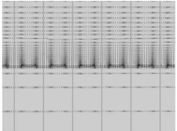
Figure 6(a). Heat flux through the microstructure in the region close to the electrodes. Almost three electrode domains are produced. Arrow length is proportional to the magnitude of the heat flux. Heat fluxes are seen to flow downwards and highest magnitudes are observed close to the electrode corners.
Figure 6(b). Heat flux through the microstructure in the region close to the electrodes. More than six electrode domains are produced. Arrow lengths are constant. Above a given height over the electrodes, the vertical component of the heat flux flips its sign and is directed upwards.
Figure 6(c). Heat flux through in the whole structure. Arrow length is constant. The role of silicon as heat spreader is apparent.
However, it is not in the temperature distribution that we are interested in, but rather in its gradient in the neighbourhood of the electrodes, as will be apparent when we consider the EHD forces acting on the medium. With regard to this point our results may claim some degree of universality, which will be clarified in the sequel. We may consider a situation in which the thermal resistance of the model is controlled by adjusting a uniform heat convection coefficient for all the outer “surfaces” of it. A value of hfilm=10 W m
-2 K-1 was chosen for this numerical experiment, which is somewhat
greater than a typical value for natural convection. Anyway, the purpose of this discussion is not a derivation of realistic final temperatures, but rather to provide an insight regarding the impact of different boundary conditions. For the sake of simplicity we have used temperature-independent thermal properties for all materials using properties at 300 K. So, boundary conditions may be described in terms of kn⋅∇T+hfilm
(
T−Text)
=0, where k is thematerial conductivity at issue and Text is an arbitrary external
temperature, for the boundaries defined by X=R, Y=Hm and Y=0.
We may compare the results obtained from this first set of boundary conditions against those from a second case, obtained from the previous one by simply switching off convection at the base of the structure. So, the second set of boundary conditions may also be written as kn⋅∇T+hfilm
(
T−Text)
=0, but only at X=R andY=Hm. Fig. 6 has been obtained with this second set of boundary
conditions. This is an interesting case study because depending on the mounting device conditions, many situations may be conceived to result in different thermal convection coefficients at every surface. Of course, if the comparison is reduced to the temperature field, this second set of boundary conditions results in a temperature increase, which almost doubles that of the first case. This is perfectly predictable from the increase of external thermal resistance. However, if what we compare is the difference in the velocity flow pattern between both situations, then relative velocity differences of less than 10% are obtained. The flow in the medium is triggered by EHD forces, which appear because of the presence of thermal gradients and electric fields, as explained in the next section. Fig. 6 is based on this second set of boundary conditions.
silicon substrate. In the medium surrounding the electrodes the dominant heat paths are directed downwards into the substrate, see Fig. 6(a). Then heat is effectively spread through the substrate, and silicon gradually gives it off upwards delivering it into the liquid in the model, as is apparent in Fig. 6(c), and downwards into the surrounding air (this latter escape path only exists in the first case considered, because in the second one convection is suppressed at the lower surface). It is precisely because of this spreading effect that in the aqueous medium around the electrodes heat paths are directed downwards in a way that is quite independent from the boundary conditions
We content ourselves with the intuition gleaned from this particular test, inasmuch as it strongly suggests that a useful understanding of the behaviour of EHD effects may be grasped without going through a painstaking study of the effects of different BCs. The calculations that follow are based on the first of the two commented sets of boundary conditions, i.e. convection takes place on all external interfaces of the system with the same convection coefficient. We want here to emphasise that although these predictions would not be exactly the same if the second case had been chosen, the general conclusions would remain valid, and the flow patterns that would be obtained in the section devoted to fluid modelling could be qualitatively hardly differentiated from those actually presented, with quantitative discrepancies of about 10% in spite of the drastic change of BCs. Of course, these differences are irrelevant for the purposes of this work.
Dynamic Thermal Effects
If the thermal problem is involved in the mechanism that sets the medium in motion, it is justifiable to study what the characteristic times that govern it are, because these should give insight into the characteristic times required for the EHD forces to be noticeable. In the case of the temperature field, the dynamics are quite slow. Times of about 102 seconds are required for the temperature to stabilise, see Fig. 7 (but this strongly depends on the boundary conditions). We have chosen three points over the electrode in the aqueous medium at different heights: L/10, L/2 and
1.75*L over the SiO2 surface, where L is the characteristic electrode
domain length i.e. electrode width plus gap. Fig. 7 shows the evolution of normalised temperature increases (i.e. temperature increase divided by the steady-state value, which is 0.6586, 0.6616 and 0.6614 K, respectively). The fourth curve in Fig. 7 produces the results from the lumped-capacitance model (Incropera and De Witt, 1996): ∆ ∆
( )
tτT
T = − −
∞ 1 exp , where the left-hand side is the
normalized temperature increase and
τ
is a characteristic time (109.1 s in our model) accounting for the thermal capacitance in the model, whose main contributors are water and silicon, and the thermal resistance associated with the convective boundary conditions. A necessary condition for the validity of this approximation is that the thermal resistance associated with the conductive heat paths is much lower than the thermal resistance associated with the external boundary conditions. This ratio is the meaning of the Biot number, which, when much smaller than 1, entails a large degree of uniformity of the temperature field, which is confirmed by the simulations. A detailed discussion on a rigorous estimate of the Biot number would require some additional disquisition because even in so simple a problem as ours there are several length scales involved. On top of that, the lumped-capacitance model may only be expected to be applicable for time scales much larger than the time required for an effective heat spreading from the electrode region into the whole model. This timescale may be estimated to be at least
water c
diff L α
τ = 2 , involving
as length scale the height of the water domain (200 µm) and the thermal diffusivity of water, yielding an estimate of 0.3 s.
1.00E-09 1.00E-08 1.00E-07 1.00E-06 1.00E-05 1.00E-04 1.00E-03 1.00E-02 1.00E-01 1.00E+00
1.E-06 1.E-05 1.E-04 1.E-03 1.E-02 1.E-01 1.E+00 1.E+01 1.E+02 1.E+03
Time (s)
N
o
rm
a
li
z
ed
t
em
p
er
a
tu
re
i
n
cr
ea
se
Height = L/10 Height = L/2 Height = 1.75 * L Lumped model
Figure 7. Dynamic evolution of the normalised temperature increase (thermal increase divided by the steady-state value) at three different points over an electrode. The fourth curve is the lumped-capacitance model prediction.
1.00E-04 1.00E-03 1.00E-02 1.00E-01 1.00E+00 1.00E+01
1.E-06 1.E-05 1.E-04 1.E-03 1.E-02 1.E-01 1.E+00 1.E+01 1.E+02 1.E+03
Time (s)
N
o
rm
al
iz
e
d
t
e
m
p
era
tu
re
g
rad
ie
n
t
Height = L/10 Height = L/2 Height = 1.75*L
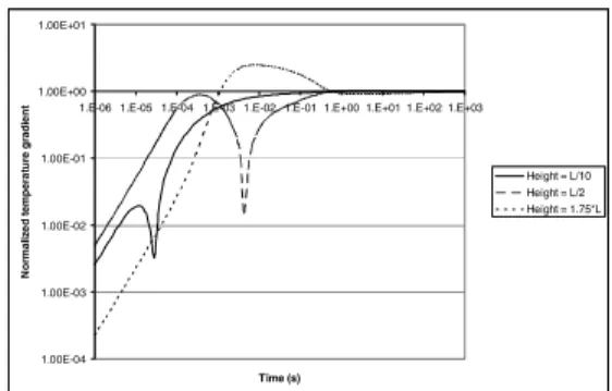
Figure 8. Dynamic evolution of the normalised magnitude of the thermal gradient at the same three points as in Fig. 7.
However, as far as EHD effects are concerned, it is the thermal gradient that deserves our attention; and to be more precise, the thermal gradient in a neighbourhood of the electrodes, for the electric fields should also be appreciable for the EHD forces to be significant. A chart of the normalised module of the themal gradient may be seen in Fig. 8 (module divided by the steady-state value, which is 7.71E-04, 1.52E-04 and 4.48E-05 K µm-1 for the same three points as in Fig. 7). Now a time close to one second is enough for these gradients to stabilise. This is an indication that once a DEP device is switched on, EHD effects are triggered within a delay that is much shorter than that associated with the temperature field.
Fluid Model Simulation
EHD Forces Background
In this subsection we resort to the analysis contained in Ramos
et al., (1998). To be brief, we produce below the final expression for
the EHD force per unit volume.
(
1)
0(
0)
02 0
2 1
E E E
E E
fehd=− ∇ε + ∇⋅ ε + ∇ε ⋅
(20)
T K
T K
∇ ⋅ ≈
∇
∇ ⋅ −
≈ ∇
− −
1 1
% 2
% 4 . 0
σ σ ε
ε
(21)
which embodies the sources of inhomogeneities in the medium. E1
is the first-order correction to the electric field attributable to the aforementioned inhomogeneities, from which we only need calculate its divergence. In order to work out this correction, it is necessary to solve an ordinary differential equation for every space point:
(
)
t
t ∂
∂ ⋅ ∇ − ⋅ ∇ − = ⋅ ∇ + ∂
⋅ ∇ ∂
⋅ 0
0 1
1 E E E
E
ε σ
σ
ε (22)
The right-hand side of Eq. (22), the source term to the dynamical equation for the correction of the divergence of the electric field, is obtained from an electrostatic FEM analysis as explained subsection “General field-modelling procedure by FEM”, which permits us to calculate the components of the field E0, and
from the thermal FEM simulations of section “Thermal modelling”, which are required for the calculation of the gradients of the
permittivity and the conductivity of the medium. Eq. (22) may be analytically solved and is uniquely determined by imposing that
1 E
⋅
∇ be periodic in time. Now we may substitute this result into Eq. (20) and derive an expression for the force per unit volume acting on the liquid.
Fluid motion can be described in terms of the Navier-Stokes equation. However, as it was outlined by the order-of-magnitude calculations computed in Ramos et al., (1998), for the case of liquid motion in dielectrophoretic microdevices the Reynolds number is very small. According to this remark, the non-linear (inertial) terms of the Navier-Stokes equation may be confidently dropped.
Some possible limitations of this approximation to the EHD forces are also discussed in Ramos et al., (1998). In particular it should be pointed out that it may fail at low frequencies if “electro-osmotic” effects are not considered. We also want to point out that the mechanical load for the Navier-Stokes equation has been obtained by averaging the result of Eq. (20) over a period of the signal. A necessary condition for the validity of this averaging is that the typical fluid velocity multiplied by the period of the signal is much shorter than L or a characteristic length for the variation of the time-averaged force field, but this condition is satisfied for the signal frequencies and amplitudes we have considered in this work.
Flow Modelling
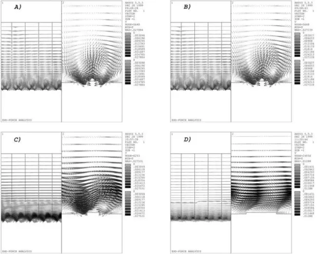
Figure 9. This figure sequence shows the fluid motion behaviour at the following frequencies: a) 10 kHz, b) 100 kHz, c) 1 MHz and d) 10MHz. On the left-hand-side figures a few electrode domains are shown, while on the right-left-hand-side ones a zoom of the neighbourhood of an electrode is represented. The applied voltage was 1 volt in a liquid of σσσσ1= 0.01 S m-1
and εεεε1= 80. Velocity values are given in µµµµm s-1
The fluid model is geometrically identical to the thermal model, reduced to its elements of water. The fluid velocity satisfies the non-slip condition at all the boundaries of the model. This corresponds to a situation where the fluid is completely enclosed and covered by a lid.
The fluid motion velocity scales like the fourth power of the applied signal amplitude because the EHD force also scales this way. Such a scaling law allows us to have a quick look at the fluid velocity in the structure by solving the model only once for any amplitude value of the applied signal. For an electrode width and separation of 20 µm (our study case), and a signal amplitude of 1 volt applied to an electrode array covered by water (i.e. ρm = 103 kg
m-3, η = 10-3 kg m-1s-1, σ1= 0.01 S m-1 and
ε
1= 80), typical fluidvelocities of around 0.025 µm s-1 are obtained, which are completely negligible compared to usual particle velocity values. If the voltage rises to 5 volts, common fluid velocities increase up to 16 µm s-1, which in many cases may be important as compared to that of the particle “free-fall” sedimentation velocity. In this case the particle may be dragged by the fluid stream or its velocity can be slowed down, depending on whether the particle moves in the same direction as the fluid or opposing it. Furthermore, if the driven
voltage is set to 10 volts, the liquid velocity will be around 250 µm s-1, which cannot be ignored at all. As can be seen, increasing the
supplied voltage in a moderate way will cause a dramatic influence on the microdevice fluid motion pattern. In fact, such high velocity, as that described in the last case, will largely dominate the particle motion behaviour.
Another parameter that affects the EHD force and also the fluid pattern motion is the frequency of the applied signal. At low frequencies, see Figs. 9(a) and 9(b), the flow pattern is almost equal to that observed in the c-DEP case, i.e. the fluid motion consists of a couple of whirlpools rotating in opposite directions; while the left one spins counter-clockwise, the other one rotates clockwise.
As the frequency increases, see Fig. 9(c) (frequency = 1 MHz), the whirlpools are highly suppressed and the flow develops a continuous stream over the electrode surface with the same direction as that of the applied travelling-wave electrical field. Figure 9(d) (frequency = 10 MHz) shows that the uniformity of the flow pattern increases with frequency. Nevertheless, the observed velocity magnitude is reduced as compared with Fig. 9(c). Inverting the signal supply sequence causes the fluid motion direction also to be inverted.
Discussion
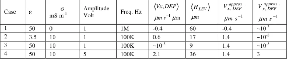
Table 1 Results for the particle motion for several particle property values, signal amplitude and frequency. <VX,DEP> stands for the average x-component of the velocity induced by DEP.<HLEV > is the average levitation
height over the electrodes. Additionally we list the estimate of the x-component of the velocity as discussed in section “Analytical estimation of the DEP force” (Eq. (17)) and also the typical value of the fluid velocity field induced by EHD effects as calculated in section “flow modelling”, which has not been taken into account for the calculation of the trajectory of the particle.
Case ε σ
mS m-1
Amplitude
Volt Freq. Hz m
,
1µ
µms− DEP Vx
m HLEV
µ 1
. ,
−
s m VxapproxDEP
µ 1
. ,
−
s m VxapproxDEP
µ
1 50 0 1 1M -0.4 60 -0.4 ~10-3
2 3.5 10 1 100K 0.6 17 1.4 ~10-3
3 50 10 1 100K ~10-3 9 1.4 ~10-3
4 50 10 5 100K 2.1 36 1.4 3
Taking advantage of these results, we may calculate the behaviour of particles in the medium exposed to both DEP and fluid drag forces. Furthermore, the accuracy of the analytic estimate for the DEP force discussed in subsection “Analytical estimation of the DEP force”, may be tested. Thus, we have considered several study cases in a medium whose relative permittivity equals 80 and whose conductivity equals 10 mS m-1.
The particle radius is 3.4 µm and the particle density is 1.05 gr cm-3. The first case (see Table 1 below) is that of a particle with ε= 50 and σ= 0 mS m-1 in a device driven by a 1 volt square signal at
1 MHz. We obtain a trajectory with a levitation height of 60 µm and a quite uniform travelling speed of -0.4 µm s-1. The voltage is so low that the EHD-related drag force is almost negligible. In this case the prediction derived from our analytic approximation (Eq. (17)) well matches the calculated particle velocity. In contrast, if we consider a particle with ε= 3.5 and σ= 10 mS m-1 in a device driven by a 1 volt square signal at 100 kHz, case 2 in the table, EHD effects are also negligible but now the levitation height is only 17 µm, which is not big compared with the electrode domain width (40 µm). The calculated averaged travelling velocity is 0.6 µm s-1, whereas the analytic estimate predicts 1.4 µm s-1. This failure may be expected as a result of the low levitation height. A third case of a particle with
ε= 50 and σ= 10 mS m-1 in a device driven by a 1 volt square signal at 100 KHz is even more unpredictable, for after the first transient motion it is seen to stop not far from the edge of the electrode at 9 µm over it. For the sake of completeness, it is worth
studying a fourth case where the influence of a change of the driving voltage may be illustrated. That is why we have studied the same particle of the third case at the same frequency (100 KHz) when the driving square signal has amplitude of 5 volts. In this case the particle levitates at 36 µm and its speed would be 2.1 µm s-1 if EHD effects were ignored, but if these are taken into account, we see that the drag forces bring about an increment of 3 µm s-1. Needless to say that if the fluid speed scales like the fourth power of the applied voltage, then higher voltages generate situations in which DEP forces may be negligible compared to EHD effects.
Conclusions
In this study we have been able to make for the first time, to the best of our knowledge, a calculation beyond an order-of-magnitude estimation of the effect of the fluid motion on the behaviour of particles in TWD-based devices. Nevertheless, the same methodology could have been applied to other DEP-related phenomena such as c-DEP and ROT. We should like to stress the relevance of our results inasmuch as they are helpful to correctly interpret the measurements obtained in this kind of devices, especially when working at high voltages and medium conductivities.
considered the effects of a square-shaped signal, which is experimentally a widely employed choice, but is usually ignored in analytical studies. In contrast with this lack of accuracy, we have undertaken an approach which takes the effects of the presence of an infinite number of frequencies, thus motivating the introduction of a complex quantity which plays the role of the Clausius-Mosotti factor but adapted to this square-signal case.
Taking into account the symmetries and periodicity of the electric field, we have been able to fully evaluate it at any point and time through a unique static simulation of only one electrode domain. Moreover, we have justified a Fourier-transform-based analytical estimate of the electric field and of the DEP force acting on a particle, which permits us at a first glance to assess its travelling-motion velocity when the particle levitates far enough from the electrodes and the electrical properties of medium and particle are known.
The next step was a thorough investigation of the thermal features of the problem. The first issue concerned the universality of our results with respect to different boundary conditions. That is why we analysed two extreme cases, and although some quantitative influence on the medium flow was noticed, the difference was low enough (around 10%) to make us confident that our results have a great scope of validity. This reduced sensitivity to the boundary conditions may be attributed to the heat spreading action of the silicon substrate.
The second issue related to the thermal behaviour was the dynamics of the thermal field distributions. As the thermal gradients are a triggering agent of EHD forces, and they are certainly the slowest, it is worth studying their dynamics. Our investigations conclusively reveal that contrary to the temperature distribution, whose stabilisation time lies in ranges of at least several seconds, the thermal gradient distribution close to the electrodes stabilises within a second. Thus one may expect that the action of EHD forces is quite immediate once the device is energised.
All these results have been combined in the calculation of the medium flow pattern. This procedure has proved to be effective to quantitatively assess the drag forces to which the particle is exposed. Even the qualitative results are enlightening. In this respect, the flow pattern shows different shapes and velocities at different frequencies. At low frequencies whirlpools are induced tending to drag the particles towards the centre of the electrodes, while at progressively higher frequencies these whirlpools vanish giving rise to an almost flat liquid stream.
Making good use of the these results, it was possible to calculate the behaviour of particles in the medium exposed to both DEP and fluid drag forces, showing that if the particle levitates high enough, the analytic estimate for the DEP force well matches the numerically calculated particle velocity. But depending on the electrical properties of the test particle, its behaviour can become unpredictable compelling the use of the numerical approach instead of the analytic one in order to obtain more reliable results.
To sum up, although the effect of DEP-related particle behaviour may be entangled with EHD effects, we have shown that all these phenomena and the particle trajectories may be calculated. We deem that these results should be helpful for the correct interpretation of experimental results and for gaining insight into a more precise design of DEP-based devices.
Appendix
In this appendix we produce the expressions for the real and imaginary parts of the modified Clausius-Mosotti factor to be applied in the case of TWD applications with four square signals shifted in time 90º from each other.
(
)
− − − − + = ′ − 1 2 4 2 1 1 4 2 1 4 )Re( σ σ
λ ε ε λ λT e T T K
(
)
(
)
+ − − − − + − − − − − − 4 1 2 1 2 4 4 2 4 1 1 1 1 T T T T T e e e e e λ λ λ λ λ ε ε λ σ σ (A.1)( )
− −(
−)
+ − + − = ′ − − 1 2 1 2 2 2 4 2 1 1 1 2 1 4Im ε ε
λ σ σ ε ε λ λ λ T T e e T K (A.2)
where T is the period of the applied signal, ε1 and σ1 are the
permittivity and conductivity of the medium, ε2 and σ2 are those of
the particle, and
2 1 2 1 2 2 ε ε σ σ λ + +
= is the inverse of the relaxation time
constant associated with the accumulation of charge at the surface of the particle.
This expression is derived as a by-product of the calculation of the DEP force (Eq. (14)) in the case of a square-shaped applied signal giving rise to electric fields of the form illustrated in Fig. 2(b). This calculation has two steps: the first one is the computation of the dynamic behaviour of the particle dipolar moment, and the second one is the averaging in time of Eq. (5) to arrive at Eq. (14).
The first step deserves perhaps some additional comments. If the curious reader wants to reproduce this step, he or she must first consider the following problem: work out the electric field around a sphere of radius R with permittivity ε2 and conductivity σ2
immersed in a medium with permittivity ε1 and conductivity σ1 if at
long distances (compared with R), the electric field is locally uniform and a periodic function of time, which for every point P has a variation in a period characterised by two values (E(1) and E(2))
as represented in Fig. 2(b) for a generic component. For every component of this locally uniform electric field, we may write a contribution to the scalar electric potential, which may be separated in terms of an inner region (I, the particle) and an outer region (II, the medium), as follows:
(
)
, ) , ( ) ( ) , ( ) ( ) ( 2 φ θ φ θ Ψ = Φ Ψ + = Φ − r t A r t B r t A II II I II (A.3)
where
r
is the distance from the centre of the particle to the point for which the potential is being calculated, and Ψ (θ,φ)is a proper combination of spherical harmonics of total angular momentum 1 (dipolar functions) for the component of the electric field that is being considered. The normalisation of this combination of spherical harmonics may always be so chosen that AI(t) may be identified with the component of the electric field which is being considered with a reversed sign. The solution to this problem of elementary electrodynamics leads to the following differential equation for BI(t):(2 ) () ( ) () 1 (2 ) () ( ) (), 1 1 2 2 1 3 1 2 2 1
3 B t Et R B t Et
R ε +ε &I =σ −σ − σ +σ I +ε −ε &
(A.4)
determined by imposing that BI(t) is periodic, which is the relevant solution once the early transients have vanished. But the corresponding component of the effective dipolar potential is directly given by4πε1BI(t), which completes step 1. The algebraic details of the solution to the latter differential equation are left to the reader. Incidentally, note the mathematical resemblance of the latter equation and Eq. (22), which makes the mathematical solution of one useful for the other. Once the first step, that is, the characterisation of the effective dipolar moment has been determined in terms of the electric properties of the medium and the particle and in terms of the two values of the electric field E(1) and
) 2 (
E , has been accomplished, the second step offers no further complications and leads directly to Eq. (14).
References
Fuhr, G., Müller, T., Schnelle, T., Hagedorn, R., Voigt, A. and Fiedler, S., 1994, “Radio-frequency microtools for particle and living cell manipulation”, Naturwissenschaften, Vol. 81, pp. 528-535.
Fuhr, G. and Shirley, S.G., 1998, “Biological application of microstructures”, Topics in Current Chemistry, Vol. 194, pp. 83-116.
Goater, A., Burt, J.P.H. and Pethig, R., 1997, “A combinated travelling wave dielectrophoresis and electrorotation device: applied to the concentration and viability determination of Cryptosporidium” Journal of Physics D: Applied Physics, Vol. 30, pp. L65-L69.
Green, N.G. and Morgan, H., 1999, “Dielectrophoresis of submicrometer latex spheres. 1. Experimental results”, Journal of Physical Chemistry B, Vol. 103, pp. 41-50.
Hughes, M.P., Pethig, R. and Wang, X-B., 1996, “Dielectrophoretic forces on particles in travelling electric fields”, Journal of Physics D: Applied Physics, Vol. 29, pp. 474-482.
Incropera, F.P. and De Witt, D.P., 1996, “Fundamentals of Heat and Mass Transfer”, John Wiley & Sons.
Masuda, S., Washizu, M. and Iwarade, M., 1987, “Separation of small particles suspended in liquid by nonuniform travelling field”, IEEE Transactions on Industry Applications, Vol. IA-23, No. 3, pp. 474-480.
Melcher, J. & Firebaugh, S., 1967, “Traveling-wave bulk electroconvection induced across a temperature gradient”, The Physics of Fluids, Vol. 10, pp. 1178-1185.
Müller, T., Arnold, W.M., Schnelle, T., Hagedorn, R., Fuhr, G. and Zimmermann, U., 1993, “A travelling-wave micropump for aqueous solutions: comparison of 1 g and µg results”, Electrophoresis, Vol. 14, pp. 764-772.
Müller, T., Pfennig, A., Klein, P., Gradl, G., Jäger, M. and Schnelle, T., 2003, “The potential of dielectrophoresis for single-cell experiments”, IEEE in Medicine and Biology Magazine, Vol. 22, pp. 51-61.
O’Brien, R.W., 1979, “A method for the calculation of the effective transport properties of suspensions of interacting particles”, Journal of Fluid Mechanics, Vol. 91, pp. 17-39.
Pethig, R., Burt, J.P.H., Parton, A., Rizvi, N., Talary, M.S. and Tame, J.A., 1998, “Development of biofactory-on-a-chip technology using excimer laser micromachining”, Journal of Micromechanics and Microengineering, Vol. 14, pp. 57-63.
Pohl, H.A., 1951, “The motion and precipitation of suspendoids in divergent electric fields”, Journal of Applied Physics, Vol. 22, pp. 869-871.
Ramos, A., Morgan, H., Green, N.G. and Castellanos, A., 1998, “Ac electrokinetics: a review of forces in microelectrodes structures”, Journal of Physics D: Applied Physics, Vol. 31, pp. 2338-2353.
Rosenthel, A. and Voldman, J., 2005, “Dielectrophoretic traps for single-particle patterning”, Biophysical Journal, Vol. 88, pp. 2193-2205.
Talary, M.S., Burt, J.P.H., Tame, J.A. and Pethig, R., 1996, “Electromanipulation and separation of cells using travelling electric fields”, Journal of Physics D: Applied Physics, Vol. 29, pp, 2198-2203.