PREDICTIVE CONTROL WITH MEAN DERIVATIVE BASED NEURAL
EULER INTEGRATOR DYNAMIC MODEL
Paulo M. Tasinaffo
∗Atair Rios Neto
∗∗Instituto Nacional de Pesquisas Espaciais (INPE), São José dos Campos, SP, Brasil
RESUMO
Redes neurais podem ser treinadas para obter o modelo de trabalho interno para esquemas de controle de sitemas di-nâmicos. A forma usual adotada é projetar a rede neural na forma de um modelo discreto com entradas atrasadas do tipo NARMA (Non-linear Auto Regressive Moving Ave-rage). Em trabalhos recentes a utilização de uma rede neural inserida em uma estrutura de integração numérica tem sido também considerada para a obtenção de modelos discretos para sistemas dinâmicos. Neste trabalho, uma extensão da última abordagem é apresentada e aplicada em um esquema de controle não-linear preditivo (NPC), com uma redefeed
forwardmodelando as derivadas médias em uma estrutura
de integrador numérico de Euler. O uso de uma rede neural para aproximar a função de derivadas médias, em vez da fun-ção de derivadas instantâneas do sistema dinâmico ODE, per-mite que qualquer precisão desejada na modelagem discreta de sistemas dinâmicos possa ser realizada, com a utilização de um simples integrador Euler, tornando a implementação do controle preditivo uma tarefa mais simples, uma vez que ela somente necessitará lidar com a estrutura linear de um integrador de primeira ordem na determinação das ações de controle. Para ilustrar a efetividade da abordagem proposta, são apresentados resultados dos testes em um problema de transferência de órbitas Terra/Marte e em um problema de controle de atitude em três eixos de satélite comportando-se como corpo rígido.
Artigo submetido em 02/02/2006 1a. Revisão em 14/02/2007
Aceito sob recomendação do Editor Associado Prof. José Roberto Castilho Piqueira
PALAVRAS-CHAVE: Controle Neural, Controle Preditivo
Não-Linear, RedesFeed forward, Modelagem Neural de
Sis-temas Dinâmicos, Integradores Numéricos de Equações Di-ferenciais Ordinárias.
ABSTRACT
Neural networks can be trained to get internal working mod-els in dynamic systems control schemes. This has usually been done designing the neural network in the form of a dis-crete model with delayed inputs of the NARMA type (Non-linear Auto Regressive Moving Average). In recent works the use of the neural network inside the structure of ordinary differential equations (ODE) numerical integrators has also been considered to get dynamic systems discrete models. In this paper, an extension of this latter approach, where a feed forward neural network modeling mean derivatives is used in the structure of an Euler integrator, is presented and ap-plied in a Nonlinear Predictive Control (NPC) scheme. The use of the neural network to approximate the mean derivative function, instead of the dynamic system ODE instantaneous derivative function, allows any specified accuracy to be at-tained in the modeling of dynamic systems with the use of a simple Euler integrator. This makes the predictive control implementation a simpler task, since it is only necessary to deal with the linear structure of a first order integrator in the calculations of control actions. To illustrate the effectiveness of the proposed approach, results of tests in a problem of orbit transfer between Earth and Mars and in a problem of three-axis attitude control of a rigid body satellite are pre-sented.
Feed Forward Neural Nets, Dynamic Systems Neural Model-ing, Ordinary Differential Equations Numerical Integrators.
1
INTRODUCTION
Multi layer feed forward artificial neural networks have the capacity of modeling nonlinear functions (e.g., Cybenko, 1988; Hornik et al, 1989). This property allows their ap-plication in control schemes, where an internal model of the dynamic system is needed, as is for example the case in pre-dictive control (Clarke et al, 1987a, 1987b). A commonly used way of representing the internal model of the dynamics of the system has been to design the neural network to learn a system approximation in the form of a discrete model with delayed inputs of the NARMA type (Non-linear Auto Re-gressive Moving Average) (Leontaritis and Billings, 1985a, 1985b; Chen and Billings, 1989, 1990 and 1992; Narendra and Parthasarathy, 1990; Hunt et al, 1992; Mills et al, 1994; Liu et al 1998; Norgaard et al, 2000). The neural net de-signed and trained in this way has the disadvantage of need-ing too many neurons in the input and hidden layers. In recent works, the use of a neural ordinary differential equation (ODE) numerical integrator as an approximate dis-crete model of motion, together with the use of Kalman fil-tering for calculations of control actions, was proposed and tested in the predictive control of dynamic systems (Rios Neto, 2001; Tasinaffo and Rios Neto, 2003). It was shown and illustrated with tests that artificial feed forward neural networks could be trained to play the role of the dynamic system derivative function in the structure of ODE numeri-cal integrators, to get internal models in nonlinear predictive control schemes. This approach has the advantage of reduc-ing the dimension and complexity of the neural network, and thus of facilitating its training (Wang e Lin, 1998; Rios Neto 2001). It was also shown that the stochastic nature and the good numerical performance of the Kalman filtering param-eter estimator algorithm make its choice a good one, not only to train the feed forward neural network (Singhal et al, 1989; Chandran, 1994; Rios Neto, 1997), but also to estimate the predictive control actions (Rios Neto, 2000). Its use allows considering the errors in the output patterns in the supervised training of the artificial neural networks. It also allows the possibility of giving a stochastic meaning to the weight ma-trices present in the predictive control functional.
This paper further explores the approach of combining feed forward neural networks with the structure of ordinary dif-ferential equations (ODE) numerical integrator algorithms to get dynamic systems internal models in predictive control schemes. Instead of approximating the instantaneous deriva-tive function in the dynamic system ODE model, the neural network is used to approximate the mean derivative function (Tasinaffo, 2003). This allows the use of an Euler structure
to get a first order neural integrator. In principle this mean derivative based first order neural integrator can provide the same accuracy as that of any higher order integrator. How-ever, it is much simpler to deal with, both in terms of the neural network training and of the implementation of the pre-dictive control scheme.
In what follows, in Section 2 the mathematical foundation, that supports the possibility of getting discrete nonlinear dy-namic system models using Euler numerical integrators with mean derivative functions, is presented. In Section 3 it is pre-sented a summary of the method of calculating the discrete control actions in a predictive control scheme with the use of Kalman filtering. In Section 4, results of tests in a problem of orbit transfer between Earth and Mars and in a problem of three - axis attitude control of a rigid body satellite are presented to illustrate the effectiveness of the proposed ap-proach. Finally, in Section 5 a few conclusions are drawn.
2
MEAN DERIVATIVE BASED EULER
IN-TEGRATOR AS A DYNAMIC SYSTEM
DISCRETE MODEL
2.1
Fundaments
For the sake of facilitating the understanding and of mathe-matically supporting the possibility of using a mean deriva-tive based Euler integrator as a dynamic system discrete model, in this section a summary of the results obtained by Tasinaffo (2003) are presented without demonstration. With this purpose, consider the following nonlinear autonomous system of ordinary differential equations,
˙
y=f(y) (1.a)
where,
y=[y1 y2 ... yn]T (1.b) f(y)=[f1(y) f2(y) ... fn(y)]T (1.c) Let, by definition, yij = yij(t), j=1, 2,...,n be a trajectory,
solution of the nonlinear ODE y˙ = f(y), starting from yij(to)at initial time to, that belongs to a domain of interest [yminj (to) , ymaxj (to)]n, and where yminj (to) and ymaxj (to) are finite. It is convenient to introduce the following vec-tor notation to indicate possible initial condition sets and the respective solutions of (1.a):
yio=yi(to)=[yi1(to) yi2(to) ... yin(to)]T (2.a)
where,i= 1, 2, ...,∞;and∞ is adopted to indicate that the
mesh of discrete initial conditions can have as many points as desired.
To start the mathematical background, two important results (e.g., Braun, 1983) about the solution of differential equa-tions (1.a) are considered. The first is about the existence and uniqueness of solutions and the second about the exis-tence of stationary solutions of (1.a).
Theorem 1 (T1) Let each of the functions
f1(y1, y2, ..., yn), ..., fn(y1, y2, ..., yn) have continuous
partial derivatives with respect to y1, ..., yn. Then, the
initial value problem y˙ = f(y),y(to) inside a domain of
interest[yminj , ymaxj ]n,j=1, 2,...,n,into,has one and only
one solutionyi=yi(t), inRn, from eachyi(to)initial state.
If two solutions,y = φ(t) andy = ϕ(t), have a common
point, then they must be identical.
Property 1 (P1) If y = φ(t) is a solution of (1.a), then
y =φ(t+c)is also a solution of (1.a), wherecis any real
constant.
Since, in general,yi˙ =f(yi) has not an analytical solution, it
is usual to only know a discrete approximation of yi=yi(t), in an interval [tk , tk+nt], through a set of discrete points,
[yi(t+k∆t) yi[t + (k+1)∆t] ... yi[t + (k +nt∆t)] ] ≡
[kyi k+1yi ... ], for a given∆t.
By definition, the secant given by two points kyi and k+1yi
of the curve yi(t) is the straight-line segment joining these two points. Thus, from the secants defined by the pair of points kyi1 andk+1yi
1,kyi2 andk+1yi2, ,kyin and k+1yin one can define the tangents:
tan∆tαi(t+k∆t)=tan∆tkαi=
[ tan∆tkαi1 tan∆tkαi2 ... tan∆tkαin ]T
(3.a)
tan∆tkαij=
k+1yi
j -kyij
∆t (3.b)
Property 2 (P2)If kyiis a discrete solution of yi˙ = f(yi)
and∆t6=0,tan∆tkαiexists and is unique.
Two other important theorems, which relate the val-ues of tank∆tαi and tank∆tα˙i, with the values of the
mean derivatives calculated from [ kyi k+1yi ... k+nyi] and
[ kyi k˙ +1yi ... k˙ +nyi], respectively, are the differential and˙
integral mean value theorems (e.g., Wilson, 1958; Munem et al, 1978; Sokolnikoff et al, 1966), enunciated in what follows.
Theorem 2 (T2) (Differential mean value theorem): If a
function yji(t), for j=1,2,...,n, is defined and continuous
in the closed interval [tk,tk+1] and is differentiable in the
open interval (tk,tk+1), then there is at least one t∗
k, tk<t∗
k<tk+1such that
˙
yij(t∗
k)= k+1yi
j -kyij
∆t (4)
T2 assures that given a secant of a differentiable yi(t) it is
always possible to find a point between k+1yi and kyi of the
intersection of the secant with the curve in tk and tk+1,such
that the tangent to this intermediate point is parallel to the secant. The valueyi(t˙ ∗
k) is called themean derivativeof yi(t) in [tk, tk+1].
Theorem 3 (T3) (Integral mean value theorem): If a
func-tion,yij(t), forj=1, 2,..., nis continuous in the closed interval
[tk, tk+1], then there exists at least onetxk interior to this interval, such that
y(txk)·∆t= tk +1
R
tk yi(t)·dt (5) In general t∗
k and txk are different and it is important to notice that the theorems do not tell how to determine these points.
Property 3 (P3) The mean derivativeyi(t˙ ∗
k)of yi(t)in the
closed interval[tk, tk+1]is equal totan∆tkαi, as an
imme-diate consequence of the definition of mean derivatives.
Theorem 4 (T4)The pointk+1yijof the solution of the system
of nonlinear differential equationsyi˙ =f(yi), forj=1, 2,...,n,
can be determined through the relationk+1yij = tank∆tαi·
∆t+ kyijfor a givenkyiand∆t.
Corollary 1 (C1)-The solution of the system of nonlinear
differential equations yi˙ = f(yi), at a given discrete point,
k+myi
j, forj=1, 2,...,n,can be determined, given an initial
kyi, by the relation:
k+myi
j= m - 1
P
l=0
tank+l
∆t αi·∆t+ kyij (6)
Corollary 2 (C2)For the system,yi˙ =f(yi), the following
relation is valid: tankm
·∆tαij = m1 ·
m - 1
P
l=0
tank+l
∆t αij, for
Notice that for the situation where the system of Eq. (1a) is autonomous, yi1(t1) =yi2(t2) for i1 6=i2 and t1 6= t2
implies that yi1(t1)˙ = ˙yi2(t2). This property establishes
that two trajectories ofy˙ =f(y) starting from two different initial conditions, yi1(to) and yi2(to), for i16=i2, will have
the same derivatives only if yi1(t1) = yi2(t2),even when
t16=t2.
The question remaining is if the mean derivative tank∆tαi of
the interval[kyi,k+1yi]is also autonomous, that is, time
in-variant? The properties that follow answer this question.
Property 4 (P4)Ifyi1(t)andyi2(t)are solutions ofy˙ =f(y)
starting fromyi1(to=0)andyi2(to=0), respectively, and
if yi1(to =0)=yi2(T)forT>0, thenyi1(∆t)=yi2(T+
∆t)for any given∆t.
Property 5 (P5)If yi1(t1)=yi2(t2), fori16=i2andt16=
t2,then,tan∆tαi1(t1) = tan∆tαi2(t2)for ∆t >0, that is,
tank∆tαi1is autonomous.
This result is useful since it determines that it is enough to know the values of tank∆tαi, for i=1, 2, ...,∞at to, in a
re-gion of interest [yminj , ymaxj ]n,j=1, 2,...,n, because fort>t0
they will repeat, as long the boundaries of [yminj , ymaxj ]n are observed.
Notice also that the trajectories of the dynamic system when propagated ahead will have angles kα(i) varying only in the
interval−π2 < kα(i)< π2 , which will thus be unique. When
retro propagated,π
2 < kα(i)< 34 , and thus·π kα(i) will also be unique in this case.
Theorem 5 (T5)The result of T4 is still valid when discrete
values of controlkuin each[tk, tk+1]are used to solve the
dynamic system:
˙
yi=f(yi, u) (7)
Demonstration: In this case the continuous function, f(yi,u),
with ku approximated as constant in [tk, tk+1], can be
viewed as parameterized with respect to the control variable and, thus, for any discrete interval the existence of the mean derivativeyi(t˙ ∗
k) =
k+1yi - k‘yi
∆t = tan∆tkαi is guaranteed
and the result in Eq. (6) is still valid.
2.2
Numerical Integrators with Neural
Mean Derivatives to Represent
Dy-namic Systems
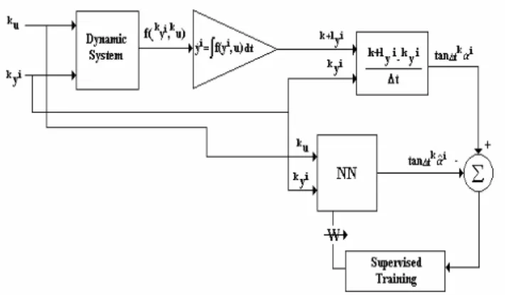
Consider the capacity of a feed forward neural network to approximate nonlinear functions (e.g., Zurada, 1992). From the previous section, one can conclude that it is possible to have a neural network to learn the mean derivatives of a given dynamical system and use them in an ODE Euler integrator structure to get a discrete representation of this system. In the proposed approach, a first possibility was adopted as il-lustrated in Fig. 1, where the neural network is trained to directly learn the dynamic system mean derivative, which is then inserted in the structure of the Euler numerical in-tegrator. In this scheme, the neural network is trained to learn the function of mean derivatives from the sampled in-put values of state kyi and control ku, with a previously fixed discrete interval∆t The value of the training output pattern tank∆tαi = k+1yi - kyi∆t is generated with the help of a nu-merical integrator of high order used to simulate one step ahead with negligible errors k+1yi, the solution of the
sys-temyi˙ =f(yi,u).
Figure 1: Supervised Training of Mean Derivatives ofyi˙ =
f(yi,u).
A second possibility that could be used, based on that adopted by Wang and Lin (1998), is depicted in Fig. 2. It is one where using the outputs of an Euler integrator the neu-ral network is indirectly trained to learn the dynamic system mean derivative. In this case, k+1ˆyi, the value of state
es-timated by the neural Euler numerical integrator, is the out-put value compared to the training pattern k+1yi to
gener-ate the error signal for the supervised training. The neu-ral network is trained to learn the function of mean deriva-tives tank∆tαi ≡tan∆tαi(ky,ku) from the values of statekyi,
control ku and of a previously fixed discrete interval∆t. In
Fig. 2, k+1yi is the value of the training pattern
to simulate the systemyi˙ =f(yi,u), and k+1ˆyi is the value
the neural network tries to estimate for k+1yi, in the
super-vised training. The relation of recurrence between kyi and k+1yi is expressed by k+1yi = tank
∆tαi·∆t+k yi, where
tank∆tαi ∼= ˆf(kyi,ku,wˆ)is the mean derivative to be approx-imated by the neural network. It should be noticed that if k+1yi is obtained from the Euler integration, then tank
∆tαi
converges to the function of derivativesyi˙ =f(yi,u). But if k+1yi is obtained from the use of a high order integrator or
experimentally, then tank∆tαi will converge to the function of
mean derivatives.
Figure 2: Supervised Training of an Euler Neural Integrator Using Mean Derivatives of.yi˙ =f(yi,u)
A correspondent algorithm to get the mean derivative based first order neural integrator would then be as follows:
1. Given in to the domains of interest
[yminj (to), ymaxj (to)]n1, j=1, 2, ..., n1, and
[umink , umaxk ]n2, k=1, 2, ..., n2, generate inside
these domains,muniformly distributed random vectors
to be the input pi,i=1, 2, ..., m,of training patterns to
the feed forward neural network.
2. Employing a high order ODE numerical integrator, propagate ahead with step size∆t the inputs pi, i=1,
2, ..., m, generating the state vectors ,i=1, 2, ..., m, at
to+ ∆t.
3. Calculate the vectorsTi to be used as training output
patterns:
Ti= ∆1t·[yi1(to+ ∆t) - yi1(to) yi2(to+ ∆t) - yi2(to) · · · yin
1(to+ ∆t) - yin1(to)]T =
[tank∆tαi1 tank∆tαi2 · · · tank∆tαin1]T=
tank∆tαiT
(8)
Notice that since the function tank∆tαi is also
au-tonomous it is only necessary propagate ahead pi,i=1,
2, ..., m, with step size∆t, to get the neural network
output patternsTi.
4. Do the supervised training of the neural network, using the patterns{(pi,Ti)}.
5. After training the neural network with a specified accu-racy, there results the dynamic system discrete model, in the form of a mean derivative based first order neural integrator:
k+1yi=tank
∆tαi·∆t+k yi (9)
Notice that using the scheme of Fig. 1, with Ti =tank∆tαi as
output patterns, avoids calculating the back propagation with k+1yi=tank
∆tαi·∆t+k yi.
To analyze the local error of this neural Euler integrator, con-sider the exact value k+1yi and the estimated value k+1ˆyi,
respectively given by Eqs. (10) and (11). k+1yi=tank
∆tαi·∆t+k yi (10)
k+1ˆyi∼=(tank
∆tαi+em)·∆t+k yi (11)
where em is the error in the output of the neural network
trained to learn the function of mean derivatives tank∆tαij
in-side a domain of interest. Due to the capacity of approxi-mation of the neural network, this error can be less than any specified value. Thus, k+1ˆyi, in Eq. (11), can have the
de-sired accuracy, since for a fixed∆t >0 the neural network is approximating inside a domain of interest the function of mean derivatives tank∆tαij that is invariant in time, and em
can be made as small as specified.
Figure 3 better illustrates this situation. Consider k+1yi,
k+1yia and k+1yie, respectively representing the exact value
of the solution of yi˙ = f(yi,u) at tk+1, the approximate
value of k+1yi obtained from a high order numerical
inte-grator, and the approximate value of k+1yi obtained from
an Euler integrator. As indicated by Fig. 3, if it is taken k+1yi =k+1 yie , in the scheme of Fig. 2, then tank
∆tαi =
ˆf(kyi,ku,wˆ)∼= f(kyi,ku), but if it is taken k+1yi=k+1 yia ,
and if k+1yie is away from k+1yi, then tank
∆tαi during the
Figure 3: Representation of mean tank∆tαi and
instanta-neoustankθi=f(kyi,ku)derivatives, foryi˙ =f(yi,u)
3
NEURAL
PREDICTIVE
CONTROL
SCHEME
The neural predictive control scheme presented in what fol-lows was proposed and demonstrated by Rios Neto (2000). In a problem of neural predictive control of a dynamic system (Mills et al, 1994), it adopts a heuristic and theoretical ap-proach to solve the problem of minimizing a quadratic func-tional subject to the constraint of a neural network predic-tor, representing the dynamics of the system to be controlled. In the proposed scheme, the problems of training the neural network and of determining the predictive control actions are seen and treated in an integrated way, as problems of stochas-tic optimal linear estimation of parameters.
The problem to be solved is that of controlling a dynamical system modeled by an ODE:
˙
y=f(y) (12)
It is assumed that the system to be controlled can be approx-imated by a discrete model. That is, for tj=t+j·∆t:
y(tj‘)∼=
f[y(tj - 1), ..., y(tj - ny); u(tj - 1), ..., u(tj - nu)]
(13)
where, y(t), ..., y(t1 - ny) and u(t - 1), ..., u(t1 - nu) are the past system responses and control actions, respectively. In the usual neural predictive control scheme, a feed forward neural network is trained to learn a discrete model as in Eq. (13). This model is then used as an internal system response model to get the smooth control actions that will track a ref-erence response trajectory by minimizing (e.g., Clarke et al, 1987a; Clarke et al, 1987b; Liu et al, 1998) the finite horizon functional:
J=[nhP
j=1[yr(tj)
-ˆ
y(tj)]T·r - 1y (t)·[yr(tj) -ˆy(tj)]+
nh - 1
P
j=0 [u(tj) - u(tj - 1)]T
·r - 1u (t)·[u(tj) - u(tj - 1)]] / 2
(14) where, yr(tj) is the reference response trajectory at timetj;
nh is the number of steps in the finite horizon of
optimiza-tion; r - 1r (tj) and ru (tj) positive definite weighting matri-- 1 ces; yˆ(tj) is the output of the feed forward neural network
previously trained to approximate a discrete model of the dy-namic system response.
The determination of the predictive control actions can be treated as a parameter estimation problem, if the minimiza-tion of the funcminimiza-tional of Eq. (14) is seen as the following stochastic problem:
yr(tj)= ˆy(tj) +vy(tj) (15.a)
0=u(tj - 1) - u(tj - 2)+vu(tj - 1) (15.b)
E[vy(tj)]=0,E[vy(tj)·vTy (tj)]=ry(tj) (15.c)
E[vu(tj)]=0,E[vu(tj)·vTu (tj)]=ru(tj) (15.d) with, j = 1, 2, ..., nh; where ˆy(tj) =
f[ˆy(tj - 1), ...,ˆy(tj - ny); u(tj - 1), ..., u(tj - nu),w] are the outputs of the neural network which is recursively used as a predictor of the dynamic system responses in the hori-zon of optimization and it is understood that for tj - k ≤t,
ˆ
y(tj - k)are estimations or measurement of already occurred
values of outputs, in the control feedback loop; vy(tj) and vu(tj) are the uncorrelated noises for different values of tj. To solve the problem of Eqs.(15) an iterative approach is needed, where in each ith iteration a perturbation is done to get a linear approximation of Eq. (15.a):
α(i)·[yr(tj) -¯y(tj,i)]=
j - 1
P
k=0
[∂ˆy(tj).∂u(tk)]{u(tk;i)}¯ ·[u(tk,i) -¯u(tk,i)]+vy(tj)
(16) wherek starts at zero, even forj>nu, as a consequence of
ˆ
y(tj) recursively being a function of u(tj - 2), ..., u(t) through
the successive recursions starting withy(ˆtj - 1), ...,ˆy(tj - ny)
the proposed case where discrete nonlinear dynamic system models using Euler numerical integrators with mean deriva-tive functions are used); 0< α(i) ≤1 is a parameter to be
adjusted to guarantee the hypothesis of linear perturbation; and the partial derivatives are calculated either by numerical differentiation or by using the chain rule to account for the composed function situation, including the back propagation rule (see, e.g., Chandran (1994)) in the feed forward neural network that approximates the derivative function of the dy-namic system.
The formulation as a stochastic linear estimation problem in each iteration is complete if the recursion in Eq.(15.b) is taken in account:
α(i)·[ˆu(t - 1) -¯u(tl,i))]=
[u(tl,i) -¯u(tl,i)]+ Pl
k=0vu(tk
)
(17a)
l=0, 1, ..., nh - 1; i=1, 2, ..., I (17b) In a more compact notation:
Ul(t,i)≡u(tl,i) (18.a)
ˆ
Ul(t - 1)≡uˆ(t- 1) (18.b)
α(i)hUˆ(t
−1) − U¯(t, i)
i
=
U(t, i) − U¯(t, i) +Vu(t)
(18.c)
α(i)Z¯u(t, i) = Hu(t, i)U
(t, i) − U¯(t, i)
+ Vy(t)
(18.d)
where the meaning of compact variables become obvious by comparison with Eqs.(16) and (17). Applying the Kalman filtering algorithm, the following solution results in a typical iteration (Rios Neto, 2000):
ˆ
U(t, i) = ¯U(t,i)+α(i)·[U(t - 1) -ˆ U(t,i)]¯ +
k(t,i)·α(i)·[Zu(t,i) - Hu(t,i)¯ ·[U(t - 1) -ˆ U(t,i)]]¯ (19.a)
k(t,i)=
Ru(t)·HuT(t,i)·[Hu(t,i)·Ru(t)·HuT(t,i)+Ry(t)] - 1≡
[R - 1u (t)+HuT(t,i)·R - 1y (t)·Hu(t,i)] - 1·HuT(t,i)·R - 1y (t) (19.b)
¯
U(t, i+1)=U(t, i);ˆ α(i)←α(i+1); ˆU(t) = ˆ
U(t, I)
(19.c)
ˆ
Ru(t,I)=[Iu - K(t,I)·Hu(t,I)]·Ru(t) (19.d) where, i = 1, 2, ..., I; Ru(t), Ry(t) andR(t, I)ˆ are the
co-variance matrices of Vu(t), Vy(t) and (U(t,I) - U(t)), respec-ˆ
tively; and Iu is an identity matrix.
A correspondent algorithm for this predictive control scheme in a typical time steptwould then be as follows.
1. The controlu(tˆ −1) (see Eq. (18b)) is the estimated
solution from the last control step. In the ith itera-tion: the approximated estimated value of control is
¯
U(t, i) = U(t, iˆ−1); α(i) ← α(i−1); and fori=1
estimates or extrapolations of estimates of last control step are used.
2. Calculate the partial derivatives ∂
ˆ
y(tj)
∂u(tk)of Eq.(16), using
the expressions of Eqs. (1A) to (3A) of the Appendix. get Hu(t,i) andZu(t,i), in Eq. (18c).¯
3. Estimate U(t, i)ˆ with the Kalman filtering of Eqs. (19.a), (19.b). Notice that the Kalman filtering can be done either in batch or sequentially, by recursively pro-cessing component to component, in sequence. Incre-menti, and repeat steps, until theyˆ(tj) are sufficiently
close to yr(tj) according to a specified error, usually taken 3·σof vy, and when this occurs take:
ˆ
U(t) =U(t, I)ˆ (20)
4
NUMERICAL TESTS
4.1
Tests in an Earth Mars Orbit Transfer.
This is a problem of low thrust orbit transfer where the state variables are the rocket massm, the orbit radiusr, the radial
speedwand the transversal speedv, and where the control
variable is the thrust steering angleθ, measured from local
horizontal. The ODE (e.g., Sage, 1968) of this dynamic sys-tem are:
˙
m= - 0.0749 (21.a)
˙
r=w (21.b)
˙
w= v2r - µ
r2 +T·sin
θ
m (21.c)
˙
v= - w·v
r +T·cosm θ (21.d) where the variables have been normalized with:µ= 1.0, the gravitational constant;T = 0.1405, the thrust; withto = 0
andtf = 5, initial and final times, where each unit of time
is equal to58.2days. The predictive control is used on line
to produce control actions that make the spacecraft follow a reference trajectory determined off line.
dy-namics. To approximate the vector mean derivative function, a multiplayer perceptron feed forward neural network, with 41 neurons (this number of neurons can be determined only empirically) with the hyperbolic tangent as activation func-tions (λ= 2), in the hidden layer, with identity activation, in the output layer, and with input bias in the hidden and output layers, was used. This feed forward neural net was trained with a parallel processing Kalman filtering algorithm (e.g., Singhal, 1989; Rios Neto, 1997), with 3600 input – output training patterns until a mean square error of 2.4789.10−6
was reached and tested with 1400 patterns, reaching a mean square testing error of 2.7344.10−6.
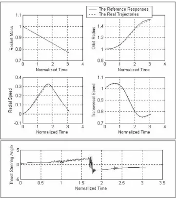
Figure 4: Predictive Control with Mean Derivatives Based Neural Euler Integrator Dynamic Model in an Earth Mars Orbit Transfer (∆t= 0.01, nh= 1).
This mean derivative neural network was then used in an Eu-ler integrator structure to produce an internal model of the orbit transfer problem dynamics to be used in a predictive control scheme where the reference was defined as the opti-mal minimum time transfer trajectory. Results obtained are shown in Figs. 4 and 5, for a discrete step size of 0.01 of normalized time (0.582 days) and receding horizons of 1 and 5 steps ahead, respectively. These results illustrate the effec-tiveness of the proposed approach when applied in this kind of problem.
Figure 5: Predictive Control with Mean Derivatives Based Neural Euler Integrator Dynamic Model in an Earth Mars Orbit Transfer (∆t=0.01, nh=5).
4.2
Tests in a Three-Axis Satellite
Atti-tude Control
In this case, the attitude control in three axes of a rigid body satellite is considered, with the correspondent dynamic equa-tions given as follows (Wertz, 1978; Kaplan, 1976):
˙ φ ˙ θ ˙ ϕ
= 1
cosθ·
cosϕ −sinϕ 0
cosϕ.cosθ sinϕ.cosθ 0 −cosϕ.sinθ −sinϕ.sinθ cosθ
·
wx
wy
wz
(22.a)
˙
wx=
I
y−Iz
Ix
·wy.wz+
Tx
Ix
˙
wy=
Iz−Ix
Iy
.wx.wz+
Ty
Iy
(22.b)
˙
wz =
I
x−Iy
Iz
.wx.wy+
Tz
where, φ, θ andϕ are the Euler angles; Ix, Iy, Iz are the
principal moments of inertia;wx,wyandwz the angular
ve-locity components, in the principal body axes;Tx,TyandTz
the control torques. The reference trajectories are defined such as to drive the Euler angles asymptotically to the origin, using updating data from navigation (Silva, 2001):
φref(tk+1) =φ(tk)·exp [−β·(tk+1−tk)] (23.a)
θref(tk+1) =θ(tk)·exp [−β·(tk+1−tk)] (23.b)
ϕref(tk+1) =ϕ(tk)·exp [−β·(tk+1−tk)] (23.c)
Initially, tests were conducted to evaluate the neural integra-tor capacity of giving an accurate discrete model of the atti-tude dynamics. To approximate the vector mean derivative function, a multiplayer perceptron feed forward neural net-work, with 20 neurons with the hyperbolic tangent as acti-vation functions (λ= 1), in the hidden layer, neurons with identity activation, in the output layer, and with input bias in the hidden and output layers, was used. This feed for-ward neural net was also trained with a parallel processing Kalman filtering algorithm, with 3200 input – output training patterns until a mean square error of 8.621.10−5was reached
and tested with 800 patterns, reaching a mean square testing error of 8.669.10−5.
This mean derivative neural network was then used in an Eu-ler integrator structure to produce the internal model of the attitude dynamics to be used in the predictive control scheme with the reference as defined in Eqs.(23) and testing data as given in Table 1. Results obtained are shown in Fig. 6.
Table 1: Testing Data
Initial Conditions: φg =
gg = gg=g2wo
ωxg = gωyg = gωzg =
g1[rpm]=π
30·1[rad/S]
Moments of Inertia: Ix = 30, Iy = 40, Iz =
20
to= 0 [s] e tf= 400 [s] β = 0.05,Ru=10−2 e
Ry=10−6
∆t1 (Neural Integrator
step size) = 0.4 [s]
∆t3(Validation Model
step size) =502[s]
Fourth Order Runge-Kutta
∆t2 (Predictive Control
Horizon) = 2 [s]
Linear Perturbation
Parameter (Eq. 16)
α= 0.15
These results illustrate the effectiveness of the proposed ap-proach when applied to this kind of problem. The oscilla-tory behavior in the y component of angular velocity may be due to the fact that the reference trajectory did not include explicitly the derivative terms corresponding to the angular regulation.
State Variables
Control Variables
Figure 6: Predictive Control with Mean Derivatives Based Neural Euler Integrator Dynamic Model in a Satellite Three-Axis Attitude Control (∆t=2 [s]; nh).
5
CONCLUSIONS
A new approach of predictive control, using a mean deriva-tive based neural Euler integrator as the internal dynamic sys-tem model, was presented. The structure of an ODE Euler numerical integrator was used to get neural discrete forward models where the neural network has only to learn and ap-proximate the algebraic and static mean derivative function in the dynamic system ODE.
The tests indicate the effectiveness of using the mean deriva-tive based neural model of the dynamic system as an internal model in the control scheme and reinforced the expected fol-lowing characteristics:
• It is a simpler task to train a feed forward neural net-work to learn the algebraic, static function of the dy-namic system ODE mean derivatives (where the inputs are samples of state and control variables), than to train it to learn a NARMA type of discrete model (where the inputs are samples of delayed responses and controls).
and number of neurons, since it does not have to learn the dynamic law, but only the derivative function.
The use of a Kalman filtering based approach to get the neu-ral predictive control actions led to results where:
• The stochastic interpretation of errors gave more real-ism in the treatment of the problem, and facilitated the adjustment of weight matrices in the predictive control functional.
• The local parallel processing version of the Kalman
fil-tering algorithm used in the control scheme exhibited efficiency and efficacy equivalent to that of the corre-spondent neural network training Kalman filtering al-gorithm. This was expected, since they are completely similar algorithms used to solve numerically equivalent parameter estimation problems.
• Only one step ahead was sufficient in the receding hori-zon of control. This feature together with the efficiency and performance of the parallel processing Kalman al-gorithms, combined with the present on board process-ing capabilities, guarantees the feasibility of real time, adaptive applications.
Notice that the proposed approach can be also be applied when an ODE mathematical model is not available. This can be done as long as dynamic system input output pairs are available to be used as training information, considering the structure of the numerical integrator with a feed forward network in place of the mean derivative function. Notice also that one could directly use an ODE numerical integrator as a dynamic system discrete model to play the role of an in-ternal model in the predictive control scheme. However, in this case one would not have the possibility of adaptive con-trol schemes, by exploring the learning capacity of the neural network and of on line updating its training.
The application of the proposed approach is not restricted to predictive control. It can be applied to any control scheme where an internal model of the controlled system is neces-sary.
Further studies shall evaluate the scheme adopted by Wang and Lin (1998), and depicted in Fig. 2. It is one where using the outputs of an Euler integrator the neural network is indi-rectly trained to learn the dynamic system mean derivative. In this paper it was only considered the scheme where the neural network is trained to directly learn the dynamic sys-tem mean derivative, which is then inserted in the structure of the Euler numerical integrator.
REFERENCES
Braun, M. (1983). Differential equations and their
appli-cations: an introduction to applied mathematics. 3rd
ed., New York: Springer-Verlag, Applied Mathemati-cal Sciences 15.
Carrara, V. (1997) Redes Neurais Aplicadas ao Controle
de Atitude de Satélites com Geometria Variável. 202p.
INPE-6384-TDI/603. Doctoral Thesis, Instituto Na-cional de Pesquisas Espaciais-INPE, São José dos Campos, 1997.
Chandran, P. S. (1994). Comments on “comparative analysis of backpropagation and the extended kalman filter for training multilayer perceptrons′′.IEEE Transactions on
Pattern Analysis and Machine Intelligence, v. 16, n. 8,
pp. 862-863.
Chen, S., Billings, S. A., Luo, W. (1989). Orthogonal least squares methods and their application to nonlinear sys-tem identification.Int. J. Control, 50(5), pp. 1873-1896.
Chen, S., Billings, S. A., Cowan, C. F. N., Grant, P. M. (1990). Practical identification of NARMAX models using radial basis function. Int. J. Control, 52(6), pp.
1327-1350.
Chen, S.; Billings, S. A. (1992). Neural networks for nonlin-ear dynamic system modeling and identification.Int. J.
Control, v. 56, n. 2, pp. 319-346.
Clarke, D.W., Mohtadi, C., Tuffs, P. S. (1987a). General-ized Predictive Control-Part I. The Basic Algorithm.
The Journal of IFAC the International Federation of
Au-tomatic Control. AuAu-tomatica, v. 23, n. 2, pp. 137-148.
Clarke, D.W., Mohtadi, C., Tuffs, P. S. (1987b). Generalized Predictive Control-Part II. Extensions and Interpreta-tions.The Journal of IFAC the International Federation
of Automatic Control. Automatica, v. 23, n. 2, pp.
149-160.
Cybenko, G. (1988). Continuous valued networks with two hidden layers are sufficient.Technical Report,
Depart-ment of Computer Science, Tufts University.
Hornik, K.; Stinchcombe, M.; White, H. (1989). Multi-layer feedforward networks are universal approxima-tors.Neural Networks, v. 2, n. 5, pp. 359-366.
Hunt, K. J.; Sbarbaro, D.; Zbikowski, R.; Gawthrop, P. J. (1992). Neural networks for control systems – A survey.Automatica, v. 28, n. 6, pp. 1083-1112.
Leontaritis, I. J., Billings, S. A. (1985a). Input-output para-metric models for nonlinear system part I: Determinis-tic nonlinear systems. Int. J. Control, 41(2), pp.
303-328.
Leontaritis, I. J., Billings, S. A. (1985b). Input-output para-metric models for nonlinear system part II: Stochastic nonlinear systems.Int. J. Control, 41(2), pp. 329-344.
Liu, G. P., Kadirkamanathan, V., Billings, S. A. (1998). Pre-dictive Control for Nonlinear Systems Using Neural Networks.Int. J. Control, v. 71, n. 6, pp. 1119-1132.
Mills, P. M., Zomaya, A. Y., Tadé, M. O. (1994). Adaptive Model-Based Control Using Neural Networks. Int. J.
Control, 60(6), pp. 1163-1192.
Munem, M. A., Foulis, D. J. (1978).Calculus with Analytic
Geometry. Volumes I and II, Worth Publishers, Inc.,
New York.
Narendra, K. S.; Parthasarathy, K. (1990). Identification and control of dynamical systems using neural networks.
IEEE Transactions on Neural Networks, v. 1, n. 1, pp.
4-27.
Norgaard, M., Ravn, O., Poulsen, N. K., Hansen, L. K. (2000). Neural Networks for Modelling and Control of Dynamic Systems. Springer, London.
Rios Neto, A. (1997). Stochastic optimal linear parameter es-timation and neural nets training in systems modeling.
RBCM – J. of the Braz. Soc. Mechanical Sciences, v.
XIX, n. 2, pp. 138-146.
Rios Neto, A. (2000). Design of a Kalman filtering based neural predictive control method. In: XIII CON-GRESSO BRASILEIRO DE AUTOMÁTICA – CBA, 2000, UFSC (Universidade Federal de Santa Catarina), Florianópolis, Santa Catarina, Brazil, CD-ROM
Pro-ceedings,pp. 2130-2134.
Rios Neto, A. (2001). Dynamic systems numerical in-tegrators control schemes. In: V CONGRESSO BRASILEIRO DE REDES NEURAIS, 2001, Rio de Janeiro, RJ, Brasil.CD-ROM Proceedings, pp. 85-88. Sage A. P. (1968). Optimum systems control. Englewood
Cliffs, NJ: Prentice-Hall, Inc..
Silva, J. A. (2001).Controle preditivo utilizando redes
neu-rais artificiais aplicado a veículos aeroespaciais. 239
p. (INPE-8480-TDI/778). Doctoral Thesis, Instituto Nacional de Pesquisas Espaciais-INPE, São José dos Campos, Brazil.
Singhal, S., Wu, L. (1989). Training Multilayer Perceptrons with the Extended Kalman Algorithm.In Advances in
Neural Information Processing Systems, VI, Morgan
Kaufman Pub. Inc., pp 136-140.
Sokolnikoff, I. S.; Redheffer, R. M. (1966). Mathematics
of physics and modern engineering. 2nd. ed., Tokyo:
McGraw-Hill Kogakusha, LTD.
Tasinaffo, P. M. (2003). Estruturas de integração neural feedforward testadas em problemas de controle predi-tivo. 230 p. INPE-10475-TDI/945. Doctoral Thesis,
In-stituto Nacional de Pesquisas Espaciais-INPE, São José dos Campos, Brazil.
Tasinaffo, P.M., Rios Neto, A. (2003). Neural Numerical Integrators in Predictive Control tested in an Orbit Transfer Problem. In: CONGRESSO TEMÁTICO DE DINÂMICA, CONTROLE E APLICAÇÕES - DIN-COM, 2, São José dos Campos: ITA, SP, Brasil,
CD-ROM Proceedings, pp. 692-702.
Wang, Y.-J., Lin, C.-T. (1998). Runge-Kutta Neural Network for Identification of Dynamical Systems in High Accu-racy.IEEE Transactions On Neural Networks, Vol. 9,
No. 2, pp. 294-307, March.
Wertz, J. R. (1978).Spacecraft attitude determination and
control. London: D. Reidel, Astrophysics and Space
Science Library, v. 73.
Wilson, E. B. (1958).Advanced Calculus. New York: Dover
Publications.
Zurada, J. M. (1992).Introduction to Artificial Neural Sys-tem. St. Paul, MN, USA: West Pub. Co.
APPENDIX: RECURRENCE RELATIONS IN
THE CALCULATION OF
H
U(
T, I
)
Equations (18.a) to (18.d) can be solved only if the matrix Hu(t,i) is known. For the case where discrete nonlinear dynamic system models using Euler numerical integrators with mean derivative functions are used, it can be calculated through the following equations (Tasinaffo, 2003):
∂k+qyi
∂ku =
∂tank+q - 1
∆t α
i
∂k+q - 1yi ·∆t+I
!
·∂k+q - 1yi
∂ku (1A)
where, q=2, 3, ..., nh.; the notation is the same as in
Sec-tion 2, andnhis the number of steps in the finite horizon of
optimization.
to (4A), in order to completely solve for Hu(t, i). u' n x y' n u' n k i y' n 2 -q k t 2 k i y' n 2 -q k t 1 k i y' n 2 -q k t u' n k i 2 2 -q k t 2 k i 2 2 -q k t 1 k i 2 2 -q k t u' n k i 1 2 -q k t 2 k i 2 -q k t 1 k i 1 2 -q k t k i 1 -q k u tan u tan u tan u tan u tan u tan u tan u tan u tan t u y ✁ ✂ ✄ ✄ ✄ ✄ ✄ ✄ ✄ ✄ ✄ ✄ ✄ ☎ ✆ ∂∂∂∂ ∂∂∂∂ ∂∂∂∂ ∂∂∂∂ ∂∂∂∂ ∂∂∂∂ ∂∂∂∂ ∂∂∂∂ ∂∂∂∂ ∂∂∂∂ ∂∂∂∂ ∂∂∂∂ ∂∂∂∂ ∂∂∂∂ ∂∂∂∂ ∂∂∂∂ ∂∂∂∂ ∂∂∂∂ ⋅⋅⋅⋅ ∆∆∆∆ ==== ∂∂∂∂ ∂∂∂∂ ++++ ∆∆∆∆ ++++ ∆∆∆∆ ++++ ∆∆∆∆ ++++ ∆∆∆∆ ++++ ∆∆∆∆ ++++ ∆∆∆∆ ++++ ∆∆∆∆ ++++ ∆∆∆∆ ++++ ∆∆∆∆ ++++ αααα αααα αααα αααα αααα αααα αααα αααα αααα ✝ ✞ ✟ ✞ ✞ ✝ ✝ (2A) y' n x y' n i y' n 1 -q k i y' n 1 -q k t i 2 1 -q k i y' n 1 -q k t i 1 1 -q k i y' n 1 -q k t i y' n 1 -q k i 2 1 -q k t i 2 1 -q k i 2 1 -q k t i 1 1 -q k i 2 1 -q k t i y' n 1 -q k i 1 1 -q k t i 2 1 -q k i 1 1 -q k t i 1 1 -q k i 1 1 -q k t i 1 -q k i 1 -q k t y tan y tan y tan y tan y tan y tan y tan y tan y tan y tan ✠ ✠ ✠ ✠ ✠ ✠ ✠ ✠ ✠ ✠ ✠ ✠ ✠ ✠ ✡ ☛ ☞ ☞ ☞ ☞ ☞ ☞ ☞ ☞ ☞ ☞ ☞ ☞ ☞ ☞ ✌ ✍ ∂∂∂∂ ∂∂∂∂ ∂∂∂∂ ∂∂∂∂ ∂∂∂∂ ∂∂∂∂ ∂∂∂∂ ∂∂∂∂ ∂∂∂∂ ∂∂∂∂ ∂∂∂∂ ∂∂∂∂ ∂∂∂∂ ∂∂∂∂ ∂∂∂∂ ∂∂∂∂ ∂∂∂∂ ∂∂∂∂ = == = ∂∂∂∂ ∂∂∂∂ + ++ + + ++ + ∆ ∆ ∆ ∆ + ++ + + ++ + ∆ ∆∆ ∆ + ++ + + ++ + ∆ ∆ ∆ ∆ + ++ + + ++ + ∆ ∆ ∆ ∆ + ++ + + ++ + ∆ ∆ ∆ ∆ + ++ + + ++ + ∆ ∆ ∆ ∆ + ++ + + ++ + ∆ ∆∆ ∆ + ++ + + ++ + ∆ ∆∆ ∆ + ++ + + ++ + ∆ ∆∆ ∆ + ++ + + ++ + ∆ ∆ ∆ ∆ α α α α α α α α α α α α α αα α α αα α α αα α α α α α α α α α α α α α α α α α ✎ ✏ ✑ ✏ ✏ ✎ ✎ (3A) u' n x y' n u' n k i y' n k t 2 k i y' n k t 1 k i y' n k t u' n k i 2 k t 2 k i 2 k t 1 k i 2 k t u' n k i 1 k t 2 k i 1 k t 1 k i 1 k t k i 1 k u tan u tan u tan u tan u tan u tan u tan u tan u tan t u y ✒ ✒ ✒ ✒ ✒ ✒ ✒ ✒ ✒ ✒ ✒ ✓ ✔ ✕ ✕ ✕ ✕ ✕ ✕ ✕ ✕ ✕ ✕ ✕ ✖ ✗ ∂∂∂∂ ∂∂∂∂ ∂∂∂∂ ∂∂∂∂ ∂∂∂∂ ∂∂∂∂ ∂∂∂∂ ∂∂∂∂ ∂∂∂∂ ∂∂∂∂ ∂∂∂∂ ∂∂∂∂ ∂∂∂∂ ∂∂∂∂ ∂∂∂∂ ∂∂∂∂ ∂∂∂∂ ∂∂∂∂ ⋅⋅⋅⋅ ∆ ∆∆ ∆ ==== ∂∂∂∂ ∂∂∂∂ ∆ ∆∆ ∆ ∆ ∆∆ ∆ ∆ ∆∆ ∆ ∆ ∆∆ ∆ ∆ ∆∆ ∆ ∆ ∆∆ ∆ ∆ ∆∆ ∆ ∆ ∆∆ ∆ ∆ ∆∆ ∆ ++++ α αα α α αα α α αα α α αα α α αα α α αα α α αα α α αα α α αα α ✘ ✙ ✚ ✙ ✙ ✘ ✘ (4A)
In this case, the back propagation is given by (e.g., Carrara, 1997; Tasinaffo, 2003):
∂yl ∂yk¯ =
∂yl ∂yk¯ +1 ·Wk
+1·I
f’(yk)¯ fork=l-1, l-2 (5A)
where,
Figure 1A– The feed forward net.
∂yl
∂yl¯ =If’(yl)¯ (6A)
I f’(yl)¯ =
f’(¯yl1) 0 0 0 0 f’(¯yl2) 0 0 0 0 . .. 0 0 0 0 f’(¯yln
k) (7A)
where the function f′(.) is the derivate of the activation
function of each neuron inside the feed forward net (Fig. 1A).
Equations 5A to 7A combined with equations (18.a) to (18.d) of Section 3 completely the problem of getting the matrix


![Table 1: Testing Data Initial Conditions: φg = gg = gg=g2w o ω x g = gω y g = gω z g = g1[rpm]= 30π · 1[rad/S] Moments of Inertia:Ix= 30, Iy= 40, I z =20 t o = 0 [s] e t f = 400 [s] β = 0.05,R u =10 − 2 e R y =10 − 6 ∆t 1 (Neural Integrator step size) = 0.](https://thumb-eu.123doks.com/thumbv2/123dok_br/18973663.454600/9.892.454.802.78.504/table-testing-initial-conditions-moments-inertia-neural-integrator.webp)
