HALF OF THRESHOLD ALGORITHM: AN ENHANCED LINEAR ADAPTIVE SKIPPING TRAINING ALGORITHM OR MULTILAYER FEEDFORWARD NEURAL NETWORKS

ISSN: 1546-9239

©2014 Science Publication

doi:10.3844/ajassp.2014.38.46 Published Online 11 (1) 2014 (http://www.thescipub.com/ajas.toc)

Corresponding Author: Manjula Devi Ramasamy, Faculty of Computer Science and Engineering, Kongu Engineering College, Perundurai-638052, Erode, India

HALF OF THRESHOLD ALGORITHM: AN ENHANCED

LINEAR ADAPTIVE SKIPPING TRAINING ALGORITHM

OR MULTILAYER FEEDFORWARD NEURAL NETWORKS

Manjula Devi Ramasamy and Kuppuswami Subbaraya Gounder

Faculty of Computer Science and Engineering, Kongu Engineering College, Perundurai-638052, Erode, India

Received 2013-09-24, Revised 2013-11-18; Accepted 2013-11-22

ABSTRACT

Multilayer Feed Forward Neural Network (MFNN) has been successfully administered architectures for solving a wide range of supervised pattern recognition tasks. The most problematic task of MFNN is training phase which consumes very long training time on very huge training datasets. An enhanced linear adaptive skipping training algorithm for MFNN called Half of Threshold (HOT) is proposed in this research paper. The core idea of this study is to reduce the training time through random presentation of training input samples without affecting the network’s accuracy. The random presentation is done by partitioning the training dataset into two distinct classes, classified and misclassified class, based on the comparison result of the calculated error measure with half of threshold value. Only the input samples in the misclassified class are presented to the next epoch for training, whereas the correctly classified class is skipped linearly which dynamically reducing the number of input samples exhibited at every single epoch without affecting the network’s accuracy. Thus decreasing the size of the training dataset linearly can reduce the total training time, thereby speeding up the training process. This HOT algorithm can be implemented with any training algorithm used for supervised pattern classification and its implementation is very simple and easy. Simulation study results proved that HOT training algorithm achieves faster training than the other standard training algorithm.

Keywords: Adaptive Skipping, Neural Network, Training Algorithm, Training Speed

1. INTRODUCTION

Multilayer Feed Forward Neural Network (MFNN) has been widely and successfully administered neural network architectures for solving supervised pattern recognition tasks (Mehra and Wah, 1992; Lippmann, 1987) due to its learning and generalization capacity. The most extensively adapted algorithm for training MFNN is Back Propagation (BPN) Algorithm. The BPN training algorithm works in two phases: Training (or Learning) Phase and Testing (Evaluation) Phase. BPN algorithm is an iterative gradient algorithm designed to find the set of weights coefficients that minimizes the total Root Mean Squared (RMS) error

measure, E, between the desired output and the actual output summed over all the training pattern input to the network Equation (1):

P p

p 1 1

E E

P =

=

∑

Ep is calculated using the following formula:

(

)

m ₂

p p p

k k

k 1 1

E t y

2 =

=

∑

where, P is the total number of training sample patterns, m is the number of nodes in the output layer p

target output of the kth node for the pth sample pattern and p

k

y is the actual output of the kth node estimated by the network for the pth sample pattern.

Although BPN algorithm has been implemented very successfully in numerous practical applications across many disciplines, it still suffers from lot of detriments. One such major detriment of the BPN training algorithm is that the training phase consumes more time than testing phase. The most important factor to be considered during the MFNN training phase is its training speed is greatly affected by the training rate, η. The training parameters that affect the MFNN training rate are dimensionality of training dataset, problem category, size of the neural network, initial weight value and training algorithm. Among these parameters, the dimensionality of training dataset is examined and the way it affects the training rate is discussed. In general, training MFNN with a bigger training data set can reduce the identifying error rate. However, ample amount of training data normally requires very long training time (Owens, 2000) which affects the training rate. Much iteration is required to train small networks for even the simplest problems. For large training data sets, it may take longer time in order to train and generalize the network well. A training algorithm that reduces this time would be of considerable value.

2. RELATED WORKS

Many researchers have investigated the above detriments and devoted their research works towards speeding up the MFNN training process through various formation ranges from different amendments of existing algorithms to evolution of new algorithms. Formation of such works include estimation of optimal initial weight (Nguyen and Widrow, 1990; Varnava and Meade, 2011), adaptation of learning rate, adaptation of momentum term (Shao and Zheng, 2009), adaptation of momentum term in parallel with learning rate adaptation (Behera et al., 2006) and using second order algorithm (Ampazis and Perantonis, 2002; Yu and Wilamowski, 2010; 2011).

First, proper initializatsion of Neural Network initial weights reduces the iteration number in the training process thereby increasing the training speed. Many weight initialization methods have been proposed for initialization of neural network weights. Nguyen and Widrow (1990) initializes the nodes’ weight within the specified range which results in the reduction of the

epoch number (Nguyen and Widrow, 1990). Varnava and Meade (2011) formulated a new initialization method by approximating the networks parameter using polynomial basis function (Varnava and Meade, 2011). Second, the learning rate is used to control the step size for reconciling the network weights. The constant learning rate secures the convergence but considerably slows down the training process. Hence several methods based on heuristic factor have been proposed for changing the training rate dynamically. Behera et al. (2006) applied convergence theorem based on Lyapunov stability theory for attaining the adaptive learning rate. Last, Second order training algorithms employs the second order partial derivatives of the error function to perform network pruning. This algorithm is very apt for training the neural network that converges quickly. The most popular second order methods employed for training are Conjugate Gradient (CG) methods, quasi- Newton (secant) methods or Levenberg-Marquardt (LM) method. Nevertheless, these methods are very computationally expensive and requires large memory. Ampazis and Perantonis (2002) presented Levenberg- Marquardt with Adaptive Momentum (LMAM) and Optimized Levenberg-Marquardt with Adaptive Momentum (OLMAM) second order algorithm that integrates the advantages of the LM and C G methods (Ampazis and Perantonis, 2002). Yu and Wilamowski (2010; 2011) modifies LM methods by rejecting Jacobian matrix storage and also replacing Jacobian matrix multiplication with the vector multiplication which results in the reduction of memory cost for training very huge training dataset.

measure with half of threshold value. By doing so, the training input samples with the actual output which are close to the target output will belong to the classified class, the remaining training input samples will belong to the mis-classified class. Only the input samples in the misclassified class are presented to the next epoch (Epoch is one complete cycle of populating the MFNN with the entire training samples once) for training, whereas the correctly classified class will be skipped for the subsequent n epochs. Thereby, the HOT algorithm dynamically reducing the number of training input pattern samples exhibited at every single epoch without affecting the network’s accuracy. Thus decreasing the size of the training input samples linearly can reduce the total training time, thereby speeding up the training process. The dominance of this HOT algorithm is that its implementation is extremely simple and easy and can lead to significant improvements in the training speed.

3. PROPOSED HOT ALGORITHM

3.1. HOT Neural Network Architecture

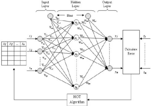
The network is furnished with n input nodes, p hidden nodes and m output nodes which are normally aligned in layers. Let P symbolized the number of training patterns. The input presented to the network is given in the form of Matrix X, with p rows and n columns. The number of network’s input nodes is equivalent to the P, column value of the input matrix, X. Each row in the Matrix X, is considered to be a realvalued vector x∈ℜn+1 which is symbolized by {x0, x1, x2,…, xn} with x0 is a bias signal. The summed realvalued vector z∈ℜp+1 generated from the hidden layer is symbolized by {z0, z1, z2, …, zp} with z0 is the bias signal. The estimated output real-valued vector y∈ℜm by the output layer is symbolized by {y1, y2, …, ym} and the corresponding target vector t∈ℜm is symbolized by {t1, t2, …, tm}. Let it signifies the itth iteration number.

The HOT algorithm that is incorporated in the prototypical MFNN architecture is sketched Fig. 1.

The network parameter symbols employed in this algorithm are addressed here. Let fN(x) and fL(x) be the nonlinear logistic activation function and linear activation function of the hidden and output layer respectively.

Since the network is fully interconnected, each layer nodes is integrated with all the nodes in the next layer. Let vij be the n×p matrix carries input-to-hidden

weight coefficient for the link from the input node i to the hidden node j and voj be the bias weight to the hidden node j. Let wjk be the p×m matrix hidden-to-output weight coefficient for the link from the hidden node j to the output node k and wok be the bias weight to the output node k.

3.2. Working Principle of HOT

The working principle of the HOT algorithm that is incorporated in the BPN algorithm is summaried below.

3.3. Weight Initialization

Step 1: Determine the magnitude of the connection initial weights (and biases) to the disseminated values within the précised range and also the learning rate, η.

Step 2: While the iteration terminating criterion is at-tained, accomplish Steps 3 through 17.

Step 3: Iterate through the Steps 4 to 15 for each input training vector to be classified whose prob

value is 1. Furnish the training pattern

Step 4: Trigger the network by rendering the training input to the input nodes in the network input layer.

3.4. Feed Forward Propagation

Step 5: Disseminate the input training vector from the input layer towards the subsequent layers. Step 6: Hidden Layer Activation net value

a) Each hidden node (zj, j = 1,2,…,p) input is aggregated by multiplying input values with the corresponding synaptic weights Equation (3):

n i i 1

inj oj ij

z (it) v (it) x (it).v (it) =

= +

∑

b) Apply nonlinear logistic sigmoid activation function to estimate the actual output for each hidden node j, 1≤ j ≤ p Equation (4):

j _zinj

1 z (it)

1 e− =

+ (4)

Attaining the differential for the aforementioned activation function Equation (5):

j

j j

(z (it))

z (it) (1 z (it)) x

∂

= × −

Fig. 1. HOT algorithm incorporated in MFNN architecture

Step 7: Output Layer Activation net value

a) Each output node (yk, k = 1,2,…,m) input is aggregated by multiplying input values with the corresponding synaptic weights Equation (6):

p

j j 1

ink ok jk

y (it) w (it) z (it).w (it) =

= +

∑

b) Apply non-linear logistic sigmoid activation function to estimate the actual output for each output node k, 1 ≤ _k ≤ _{m Equation (7):}

k _yink

1 y (it)

1 e− =

+ (7)

Attaining the differential for the afore-mentioned activation function Equation (8):

k

k k

(y (it))

y (it) (1 y (it)) x

∂ _{= × −}

∂ (8)

3.5. Accumulate the Gradient Components

Step 8: For each output unit k,1 ≤ k ≤ m, the error gradient calculation for the output layer is formulated as Equation (9):

k(it) y (it) [1 y (it)] [tk k k y (it)]k

δ = × − × − (9)

Step 9: For each hidden unit j, 1 ≤ j ≤ p, the calculation of error gradient for the hidden layer is formulated as Equation (10):

m

j j j j

k 1

jk

(it) (it).w (it) .z (it).[1 z (it)] =

 

∂ = δ  −



∑

3.6. Weight Amendment using Delta-Learning

Rule

Step 10: For each output unit.

The weight amendment is yielded by the following updating rule Equation (11):

jk jk jk

W (it 1)+ =W (it)+△W (it 1)+ (11)

The bias amendment is yielded by the following up-dating rule Equation (12):

ok ok ok

W (it 1)+ =W (it)+△W (it 1)+ (12)

Step 11: For each hidden unit.

The weight amendment is yielded by the following updating rule Equation (13):

ij ij ij

The bias amendment is yielded by the following up-dating rule Equation (14):

oj oj oj

V (it 1)+ =V (it)+ ∆V (it) (14)

3.7. HOT Algorithm Steps

Step 12: Measure the dissimilarity between the target and true value of each input sample (xi, i = 1,2,…,n) which imitates the utter error value Equation (15):

k k

t −y (it) , k=1, 2,..., m (15)

Step 13: Accomplish collation between the utter error value |tk-yk| and half of error threshold,

dmax/2. k k

max

d t y (it)

2

− < . If so, Goto Step 14.

Else Goto Step 16.

Step 14: Compute the possibility value for presenting the input sample in the next iteration:

i

i

if x is classified correctly and 0,

prob (x ) number of epoch is less t than n

1, otherwise   =  

Step 15: Calculate n, number of epochs to be skipped a) Initialize the value of n to zero for a particular sample xi

b) If xi is classified correctly, then increment n value by c, where c → Linear Skipping Factor. Step 16: Construct the new probability-based training

dataset to be presented in the next epoch. Step 17: Inspect for the halting condition such as

applicable Root Mean Square error (RMS), elapsed epochs and desired accuracy.

4. RESULT ANALYSIS

In Section 4, the proposed HOT algorithm has been analyzed for the categorization problem concomitant with two-class and multi-class. The real-world workbench data sets applied for training and testing are Iris, Waveform, Heart and Breast Cancer Data Set which are consumed from the University of California at Irvine (UCI) Machine Learning Repository (Asuncion and Newman, 2007). The concrete quantity of the data sets used is provided in the Table 1.

The initial values of the weights coefficients are chosen randomly between -0.5 and +0.5 using the Nguyen-Widrow (NW) initialization method for faster learning. All the bias nodes are enforced with the unit value.

4.1. Multiclass Problems

4.1.1. Iris Data Set

The Iris flowering plant database consists of measurements of 150 flower samples. For each flower, the four facets weighed are positioned here: Sepal Length and Width and Petal Length and Width. In fact, these four facets are involved in the categorization of each flower plant into apposite Iris flower genus: Iris Setosa, Iris Versicolour and Iris Virgincia. The 150 flower samples are equally scattered amidst the three iris flower classes. Iris setosa is linearly separable from the other 2 genus. But Iris Virgincia and Iris Versicolour are nonlinearly detachable. Out of these 150 flower samples, 90 flower samples are employed for training and 60 flower samples for testing.

4.1.2. Waveform Data Set

The Waveform database generator data set contains 5000 wave’s samples measurement. The 5000 wave’s samples are equally distributed, about 33%, into three wave families (Asuncion and Newman, 2007). Each wave’s samples are recorded using 21 numerical features. Among these 5000 wave’s samples, 4800 waves are randomly selected for training and 200 waves for testing.

4.2. Two-Class Problems

4.2.1. Heart Data Set

The Statlog Heart disease database consists of 270 patient’s samples. Each patient’s characteristics recognized with the 13 numerical attributes. These 13 features are involved in the detection of the presence and absence of heart disease for the patients.

4.2.2. Breast Cancer Data Set

The Wisconsin Breast Cancer Diagnosis Dataset contains 569 patient’s breasts samples among which 357 diagnosed as benign and 212 diagnosed as malignant class. Each patient’s breast cancer are detected using the 32 numerical features.

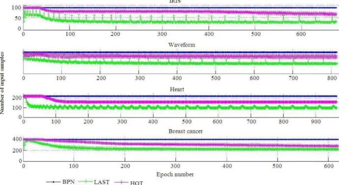
Fig. 2. Epoch-wise training input samples for all datasets

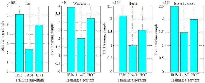
Fig. 4. Total Training samples taken by BPN, LAST and HOT algorithm during the training phase

Fig. 5. Total training time taken by BPN, LAST and HOT algorithm Table 1. Concrete quantity of the data sets

Datasets No. of Attributes No. of Classes No. of Instances

Iris 4 3 150

Waveform 21 3 5000

Heart 13 2 270

Breast Cancer 31 2 569

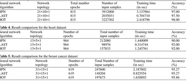
Table 2. Result Comparison for the IRIS dataset

Neural network Network Number of Total number Training time Accuracy algorithm topology epochs of input samples (in sec) (%)

BPN 4×5×1 675 60750 0.887442 91.67

LAST 4×5×1 675 24148 0.288156 91.67

Table 3. Result comparison for the waveform dataset

Neural network Network Total number Number of Training time Accuracy

Algorithm topology epochs input samples (in sec) (%)

BPN 21×10×1 815 3912000 3.137964 97.00

LAST 21×10×1 815 2035031 0.704710 97.50

HOT 21×10×1 815 3227302 2.418796 98.00

Table 4. Result comparison for the heart dataset

Neural network Network Number of Total number of Training time Accuracy

algorithm topology epochs input samples (in sec) (%)

BPN 13×5×1 964 212080 1.440009 90.00

LAST 13×5×1 964 98976 0.314744 92.00

HOT 13×5×1 964 157833 1.245761 92.00

Table 5. Result comparison for the breast cancer dataset

Neural network Network Number of Total Number of Training time Accuracy

algorithm topology epochs input samples (in sec) (%)

BPN 31×15×1 619 247600 2.187802 95.27

LAST 31×15×1 619 148204 0.825554 95.27

HOT 31×15×1 619 197673 1.638892 95.86

The consolidated simulation results of BPN, LAST and HOT algorithm are furnished in Table 2-5, which notify the Training Samples, Training Time and Accuracy. From this table, the HOT algorithm achieves higher or equal accuracy rate than BPN and LAST and also, it yields improved computational training speed in terms of the total number of trained input samples as well as total training time over BPN and less than LAST.

4.2.3. Result Comparison

From the Table 2-5, it is concluded that the proposed HOT algorithm attains the higher training performance in terms of trained input samples and time compared to BPN. The comparison results of the total training samples and total training time attained by the BPN, LAST and HOT algorithm for the above mentioned dataset are consolidated in Fig. 4 and 5. From this Fig. 4, it is portrayed that the total number of training samples consumed by HOT algorithm is reduced by an average of nearly 43% of BPN algorithm. Whereas, the LAST algorithm is reduced to an average of nearly 60% of BPN algorithm since the error value is compared with the half of maximum threshold.

Thus decreasing the size of the trained input samples can reduce the training time which is shown in the following Fig. 4, thereby increasing the speed of the training process without affecting the accuracy.

From the Fig. 5, the total training time of HOT algorithm is reduced to an average of nearly 20-40% of BPN algorithm for various datasets.

5. CONCLUSION

The research paper concludes that a new and simple Half of Threshold (HOT) algorithm for the training of Multilayer feed forward neural networks improves the training speed by skipping the correctly classified input samples. The performances of the proposed HOT algorithms are compared with BPN and LAST algorithm on four benchmark function approximation problems: IRIS, Waveform, Heart and Breast Cancer. The comparisons are made in terms of total number of training input samples and computational time required for training. It is found that the proposed HOT algorithm is much faster than the standard BPN algorithm and slower than LAST algorithm to attain the same accuracy.

The simulation of all the above mentioned algorithm are done using the machine with the processor model Intel® Core I5-3210M, CPU speed of 2.50GHz and 4 GB of RAM. The software used for simulation is MATLAB with the version R2010b.

6. REFERENCES

Ampazis, N. and S.J. Perantonis, 2002. Two highly efficient second-order algorithms for training feedforward networks. IEEE Trans. Neural Netw., 13: 1064-1074. DOI: 10.1109/TNN.2002.1031939 Asuncion, A. and D.J. Newman, 2007. UCI Machine

Behera, L., S. Kumar and A. Patnaik, 2006. On adaptive learning rate that guarantees convergence in feedforward networks. IEEE Trans. Neural Netw., 17: 1116-1125. DOI: 10.1109/TNN.2006.878121

Devi, R.M., S. Kuppuswami and R.C. Suganthe, 2013. Fast linear adaptive skipping training algorithm for training artificial neural network. Math. Problems

Eng., 2013: 346949-346957. DOI:

10.1155/2013/346949

Lippmann, R.P., 1987. An introduction to computing with neural nets. IEEE ASSP Mag., 4: 4-22. DOI: 10.1109/MASSP.1987.1165576

Mehra, P. and B.W. Wah, 1992. Artificial Neural Networks: Concepts and Theory. 1st Edn., IEEE Computer Society Press, Los Alamitos, ISBN-10: 0818689978, pp: 667.

Nguyen, D. and B. Widrow, 1990. Improving the learning speed of 2-layer neural networks by choosing initial values of the adaptive weights. Proceedings of the IJCNN International Joint Conference on Neural Networks, Jun. 17-21, IEEE Xplore Press, San Diego, CA, USA., pp: 21-26. DOI: 10.1109/IJCNN.1990.137819

Owens, J.A., 2000. Empirical modeling of very large data sets using neural networks. Proceedings of the IEEE-INNS-ENNS International Joint Conference on Neural Networks, Jul. 27-27, IEEE Xplore Press, Como, pp: 302-307. DOI: 10.1109/IJCNN.2000.859413

Shao, H. and G. Zheng, 2009. A new BP algorithm with adaptive momentum for FNNs training. Proceedings of the WRI Global Congress on Intelligent Systems, May 19-21, IEEE Xplore Press, Xiamen, pp: 16-20. DOI: 10.1109/GCIS.2009.136

Varnava, T.T. and A.J. Meade, 2011. An initialization method for feedforward artificial neural networks using polynomial bases. Adv. Adaptive Data Anal., 3: 385-400. DOI: 10.1142/S1793536911000684 Yu, H. and B.M. Wilamowski, 2010. Improved

computation for levenberg marquardt training. IEEE Trans. Neural Netw., 21: 930-937. DOI: 10.1109/TNN.2010.2045657