Application of a Mobile Robot to Spatial Mapping of Radioactive Substances in Indoor Environment

(1)

Application of a Mobile Robot to

Spatial Mapping of Radioactive

Substances in Indoor Environment

Luis Fernando Piardi

Dissertation presented to the School of Technology and Management of Bragança to obtain the Master Degree in Engenharia Industrial.

Work oriented by:

Professor PhD José Luis Sousa Magalhães Lima Professor PhD Paulo Costa

Professor PhD Marcos Bombacini

(2)

(3)

Application of a Mobile Robot to

Spatial Mapping of Radioactive

Substances in Indoor Environment

Luis Fernando Piardi

Dissertation presented to the School of Technology and Management of Bragança to obtain the Master Degree in Engenharia Industrial.

Work oriented by:

Professor PhD José Luis Sousa Magalhães Lima Professor PhD Paulo Costa

Professor PhD Marcos Bombacini

(4)

(5)

Acknowledgement

I would like to express my thanks to Professor PhD José Luis Lima, supervisor of this work, for the dedication, guidance, incentive and opportunity to develop this work, and articles, highlighting the challenge and support to develop the writing of the document in English.

To Professor PhD Paulo Costa, co-supervisor of this work, my gratitude for the guid-ance and willingness to share his vast knowledge in the area.

To Professor PhD Ana Isabel Pereira, for support, availability and supervision in work activities using evolutionary algorithms.

To Professor PhD Marcos Bombacini for having accepted to be the distance co-supervisor in this agreement of the Dual Diplomacy program.

To my friends and college colleagues, Dual Diplomacy, laboratory and calculus center which I shared eternal moments of learning.

I thank the IPB, UTFPR and INESC-TEC for the conditions provided.

Finally, a special thanks to my parents and family for having provided all the accom-paniment and support necessary to carry out this work.

(6)

(7)

Abstract

Nuclear medicine requires the use of radioactive substances that can contaminate critical areas (dangerous or hazardous) where the presence of a human must be reduced or avoided. The present work uses a mobile robot in real environment and 3D simulation to develop a method to realize spatial mapping of radioactive substances. The robot should visit all the waypoints arranged in a grid of connectivity that represents the environment. The work presents the methodology to perform the path planning, control and estimation of the robot location. For path planning two methods are approached, one a heuristic method based on observation of problem and another one was carried out an adaptation in the operations of the genetic algorithm. The control of the actuators was based on two methodologies, being the first to follow points and the second to follow trajectories. To locate the real mobile robot, the extended Kalman filter was used to fuse an ultra-wide band sensor with odometry, thus estimating the position and orientation of the mobile agent. The validation of the obtained results occurred using a low cost system with a laser range finder.

Keywords: Mobile Robot; Spatial Mapping Radioactive Substances; Path Planning; Genetic Algorithm; Kalman Filter; Ultra-wide Band; Laser Range Finder.

(8)

(9)

Resumo

A medicina nuclear requer o uso de substâncias radioativas que pode vir a contaminar áreas críticas, onde a presença de um ser humano deve ser reduzida ou evitada. O presente trabalho utiliza um robô móvel em ambiente real e em simulação 3D para desenvolver um método para o mapeamento espacial de substâncias radioativas. O robô deve visitar todos os waypoinst dispostos em uma grelha de conectividade que representa o ambiente. O tra-balho apresenta a metodologia para realizar o planejamento de rota, controle e estimação da localização do robô. Para o planejamento de rota são abordados dois métodos, um baseado na heurística ao observar o problema e ou outro foi realizado uma adaptação nas operações do algoritmo genético. O controle dos atuadores foi baseado em duas metodolo-gias, sendo a primeira para seguir de pontos e a segunda seguir trajetórias. Para localizar o robô móvel real foi utilizado o ﬁltro de Kalman extendido para a fusão entre um sensor ultra-wide band e odometria, estimando assim a posição e orientação do agente móvel. A validação dos resultados obtidos ocorreu utilizando um sistema de baixo custo com um laser range finder.

Palavras-chave: Robô móvel; Mapeamento Espacial de Substâncias Radioativas; Plane-jamento de Caminho; Algoritmo Genético; Controle; Filtro de Kalman; Ultra-wide Band, Laser Range Finder.

(10)

(11)

List of Tables

2.1 Solution for the TSP exempliﬁed in Figure 2.23. . . 30

3.1 Dimensions of real WMR . . . 36

3.2 Sensor laser rangeﬁnder URG-04LX speciﬁcation [74] . . . 52

5.1 Data used in GA to path planning . . . 78

5.2 Path planning time for a 5X5 connectivity grid . . . 78

5.3 Number of waypoints visited by path planning algorithms considering a 5X5 connectivity grid. . . 79

5.4 Heuristic and GA method comparison (visited cells). . . 83

5.5 Time consumed for the path planning algorithm to converge. . . 84

5.6 Dimension of the connectivity grid for controller tests in simulation. . . . 85

5.7 Controller parameters waypoint path in simulation. . . 86

5.8 Controller parameters segment based path in simulation. . . 87

5.9 Evaluation of controller errors in simulation environment . . . 89

5.10 Dimension of real environment for tests with real robot. . . 90

5.11 Location of Pozyx anchors. . . 91

5.12 Waypoint path controller parameters in real environment . . . 92

5.13 Controller parameters segment based path in Real Environment . . . 94

5.14 Evaluation of controller errors in real environment . . . 95

(16)

(17)

List of Figures

1.1 PET procedure [1]. . . 2

2.1 Robots used for inspection at Fukushima plant after disaster [8]. . . 7

2.2 SIAR robot conducting an inspection in a sewer[10]. . . 8

2.3 SACI robot emitting a jet of water to combat the ﬁre [11]. . . 8

2.4 Soryu robot navigating through wreckage in test environment [12]. . . 9

2.5 The Roomba discovery vacuum [5]. . . 10

2.6 Curiosity - Robot for exploration of the planet Mars (NASA). (Adapted from:[14]). . . 10

2.7 Geometry of robotic locomotion Ackerman steering. . . 12

2.8 Geometry of robotic locomotion omnidirectional [17]. . . 12

2.9 Omni wheel with six free rotating rollers mounted around the wheel rim [20]. 13 2.10 Robot with diﬀerential drive (Pioneer P3-DX). . . 14

2.11 Localization and navigation system based on wire guidance [25]. . . 15

2.12 Localization and navigation system based on strip guidance [25]. . . 16

2.13 Localization and navigation system based on marker [25]. . . 16

2.14 Localization and navigation system based on trilateration and triangulation [25]. . . 18

2.15 Visibility Graph: the highlighted line indicates the selected path for this example. [4] . . . 21

2.16 VoronoiGraph [4]. . . 21

(18)

2.18 Progress (from the left to the right ﬁgure) of the RRT algorithm to ﬁnd

the path by connecting the desired points [20]. . . 23

2.19 PRM algorithm [35]. . . 24

2.20 Potential ﬁeld algorithm [35]. . . 25

2.21 Local minima present in potential ﬁeld, forming a trapped path [35]. . . 26

2.22 Example of a path generated by algorithm A* (adapted from [47]). . . 27

2.23 Example of a travelling salesman problem. . . 29

3.1 System architecture proposed for the interaction between the user and the robot. . . 31

3.2 Interface between ControlApp and the user, highlighting its functionalities: A - Communication, B - Inserting Waypoints and C - Robot navigation area. 32 3.3 Connectivity grid where resolution of the grid is deﬁned by the user. . . 33

3.4 Communication between robot and ControlApp. . . 34

3.5 Prototype of real mobile robot. . . 35

3.6 Detail of the support structure of the robot built with aluminum extrusion proﬁle in X. . . 35

3.7 Robot in the plane representing the global robot reference frame. . . 37

3.8 Example of a restricted motion for a mobile robot with diﬀerential drive. . 38

3.9 Mobile robot electronic architecture. . . 39

3.10 Raspberry Pi model B. . . 40

3.11 Arduino Uno. . . 41

3.12 Connection between Pozyx tag and Arduino (adapted from [62]). . . 41

3.13 Connection between Arduino, CNC shild V3 and chip Allegro MicroSys-tems A4989. . . 42

3.14 Interface of Pozyx system tag to connect at Arduino [62]. . . 43

3.15 Overview of SimTwo simulator tabs and tools [64]. . . 44

(19)

3.16 Simulated robot. . . 45

3.17 Pozyx tag high-level component blocks [62]. . . 48

3.18 Pozyx anchor using a power bank as energy source. . . 48

3.19 Arrangement of Pozyx anchors and tag location radius. . . 49

3.20 Laser Ranger Finder Hokuyou URG-04LX. . . 52

3.21 Laser operation and location of the robot in the ground truth approach. . . 53

4.1 Data fusion using information of Pozyx sensor and odometry (adapted from [67]). . . 56

4.2 Connectivity grid (size: 5x5) and an example of possible points and seg-ments. Without an obstacle the 12 point will be a reachable point. . . 61

4.3 Representation of the connectivity grid. . . 62

4.4 Von Neumann neighborhood with unitary radius. . . 62

4.5 Heuristic method using eight direction priorities to generate eight paths and select the smallest. . . 63

4.6 Possible chromosome that constituted the initial population of connectivity grid. . . 64

4.7 Geometry of the mask for the generation of the initial population. . . 65

4.8 Crossover operation details. . . 66

4.9 Detail of mutation operator. . . 67

4.10 Spline curve generated between three distinct waypoints, sampled in smaller parts. . . 70

4.11 Feedback control system diagram: above points following and below seg-ment following. . . 71

4.12 Considerations for robot control following points. . . 72

4.13 Reference velocity as a function of robot distance to the last trajectory point. 73 4.14 Considerations for robot control segments following. . . 74

4.15 Linear velocity as a function of angular velocity. . . 75

5.1 Connectivity Grid with 25 cell. . . 78

(20)

5.4 Case A: Connectivity grid 8x8 without obstacle. . . 80

5.5 Case A: Performance of algorithms to path planning. . . 81

5.6 Case B: 8x8 connectivity grid with two obstacle. . . 81

5.7 Case B: Performance of algorithms to path planning. . . 82

5.8 Case C: 8x8 connectivity grid with three obstacle. . . 82

5.9 Case C: Performance of algorithms to path planning. . . 83

5.10 Path executed in environment with unknown obstacles. . . 85

5.11 Control follow point with measurement noise and uncertainty of sensor Pozyx. 86 5.12 Comparison between spline trajectory and path realized by simulated robot with point following controller. . . 87

5.13 Segment following controller with measurement noise and uncertainty of sensor Pozyx. . . 88

5.14 Comparison between spline trajectory and path realized by simulated robot with segment following controller. . . 88

5.15 Indoor environment layout developed for testing with real robot. . . 90

5.16 Region Labeling of ground truth. . . 91

5.17 Ground truth and anchors distributed in real test environment. . . 92

5.18 Waypoint path controller results in real environment. . . 93

5.19 Segment based path controller results in real environment. . . 94

B.1 Petri Net: software application embedded in the robot to act on the wheels, communicate with ControlApp and perform the location by the Extended Kalman Filter (EKF). . . 110

C.1 Flowchart to accomplish path planning considering a direction priority. There are eight direction priorities, executed one at a time. . . 112

D.1 Petri Net: unknown obstacle detected and path re-planning. . . 114

(21)

Acronyms

EKF Extended Kalman Filter.

GA Genetic Algorithm.

IDE Integrated Development Environment.

LRF Laser Range Finder.

MCU Micro-controller Unit.

NUMDAB Nuclear Medicine Database.

ODE Open Dynamics Engine.

PET Positron Emission Tomography.

PRM Probabilistic Roadmap.

RF Radio Frequency.

RFID Radio Frequency Identiﬁcation.

RRT Rapidly Random Tree.

RSS Received Signal Strength.

SIAR Sewer Inspection Autonomous Robot.

(22)

ToF Time of Flight.

TSP Travelling Salesman Problem.

UDP User Datagram Protocol.

UWB Ultra-wideband.

WMR Wheeled Mobile Robots.

(23)

Chapter 1 Introduction

This work deals with the study and development of three essential areas of wheeled mobile robot, being: path planning, location estimation and control. The intention is to develop methods to enable a mobile robot to perform spatial radiation map of an indoor envi-ronment contaminated by harmful radioactive substances to humans. As a basis for the studies, a simulation platform will be used to test the algorithms. After the simulation step, a real mobile robot will be used to validate the methodology for the environment scan.

1.1 Motivation and Framework

Nuclear medicine requires the use of radioactive substances to observe the physiological condition of human tissues in a minimally invasive manner. To diagnose diseases such as cancer and its metabolism, methods such as Positron Emission Tomography (PET) are applied. Basically the patient ingests a radioactive substance analogous to glucose, where cells that have an accelerated reproduction tend to consume it [1]. However the substance is not fully absorbed, resulting in a concentration of radiation in the region of rapid cell reproduction (usually regions where malignant cancer cells are developing). The patient then undergoes a procedure that performs a scan on his body to locate regions where the radioactive emissions are concentrated as shown in Figure 1.1a. Figure 1.1b shows the

(24)

image resulting from the diagnoses where regions of the body with abnormal cell behavior are highlighted.

(a) PET scanner. (b) Diagnos-tic.

Figure 1.1: PET procedure [1].

The administration of nuclear radio pharmaceutical components to the patient must be carefully done by specialists. Unfortunately, the patient can contaminate the environ-ment with physiologic needs. Moreover, environenviron-ment and the patient should be isolated by a period of time regarding the decay of nuclear properties. The inspection of the clearance of the environment is mainly made by human beings that are exposure to the ionizing radiation that may cause the damage in the organs and tissues. The scanning and measurement of the radiation can be done resorting to a mobile robot that performs the acquisition based on a Geiger counter. The spatial radiation map performed by the mobile robot should guarantee that the complete scan is performed and ensure the environment is clean and technicians can enter the room.

According to Nuclear Medicine Database (NUMDAB), there are 1490 nuclear medicine institutions in the world, of which 1288 are active. Actually, 690 thousand PET and PET-CT (Computed Tomography) annual examinations are registered in the world [2].

(25)

1.2. OBJECTIVES 3

1.2 Objectives

The main objective of this work is to develop and test a solution with low cost mobile robots to perform the spatial mapping of radioactive substances in indoor environments without human intervention. Consequently the other objectives also make up this work:

• Develop an interface between man and robot for remote access in real time.

• Development of methods for planning routes in a connectivity grid, visiting all available points.

• Implement a smooth curve for the robot path reference.

• Development of controllers for the robot to perform the trajectory.

• Implement the methodology developed in SimTwo simulation environment.

• Implement the methodology developed in real environment using a mobile robot provided, a location system based on UWB, and a ground truth of low cost.

1.3 Document Structure

This document is divided into 6 chapters, to describe the work carried out throughout the dissertation.

The introduction is described in Chapter 1, which presents the proposal of the work as well as the contamination of indoor environments by patients undergoing PET exams, and a mobile robot is proposed to perform the spatial mapping of the radioactive substance from nuclear medicine activities.

(26)

Chapter 3 presents the system architecture used in this work, demonstrating its struc-ture used to address the problem and presenting and describing the software, hardware and simulation environment.

Chapter 4 presents the Extended Kalman Filter to address the errors and uncertainties in the robot location, followed by the description of the heuristic and genetic algorithm for path planning. It ends with a description of two methods for controlling the robot: points following and segment following.

Chapter 5 contains the results obtained during the tests to validate the methodology and is ﬁnished with the practical results.

(27)

Chapter 2 Related Work

In this section it will be analyzed the related work in the area of wheeled mobile robots such as, real applications, geometries, localization and path planning. Bearing in mind the application developed during this work, and taking into account the current context where each day becomes more common the coexistence with the diﬀerent types of robots, this chapter tries to elaborate, based on a scientiﬁc research the state of the art.

2.1 Wheeled Mobile Robot Applied in Monitoring

and Surveillance

The first robots have emerged to operate in a cell isolated environment, most often within warehouses or industries. There is no universally recognized definition of robotics, however Russel and Norving present a possible definition as:“Robots are physical agents that perform tasks by manipulating the physical world. To do so, effector they are equipped with effectors such as legs, wheels, joints, and grippers. Robots are also equipped with sensors, which allow them to perceive their environment” [3].

In general, robots have been developed to perform tasks that the human being for rea-sons of unhealthiness, incapacity or disinterest does not execute. The developed robotic systems are usually implemented when, for the same work, the robot performs with a

(28)

higher quality and speed or at a lower cost compared to human work [4]. Citing Tzafes-tas: “The robots contribute in one or the other way to human, industrial, agricultural, technical, and social life improvements”[5].

The class of robot used in this work is of the mobile category with wheels. A Wheeled Mobile Robots (WMR) is applied to problems related to operations in complex envi-ronments such as hazardous and dangerous envienvi-ronments, unknown envienvi-ronments with dynamic obstacles, or planetary explorations and others. It will be presented the concept and advantages of applying WMR for inspection, monitoring and surveillance, and then will be exposed some examples and practical applications well respected.

Inspection and monitoring of controlled or hazardous environments is an important issue for the sustainability, maintenance and use of these sites. These environments can be characterized due to the presence of dust, humidity, large temperature variations, ﬁre risks, biological agents or even toxic and radioactive substances, which is the case addressed in the present work.

The classical approach to environment inspection and monitoring activities utilizes human workers, i.e., this activity may present safety and health hazards to human in-spectors. For this reason, there is a need to avoid and replace the presence of humans in hazardous areas by robots. Solutions with WMR have been an ideal alternative for inspection and monitoring because they have a relatively low cost, avoid worker exposure, are more accurate and perform in less time when compared to the classical approach [6].

(29)

2.1. WHEELED MOBILE ROBOT APPLIED IN MONITORING AND SURVEILLANCE7

2.1.1 Quince Robot

Quince WMR was employed to conduct inspections and monitoring of the nuclear power plant accident at Fukushima Daiichi in Japan. Due to an earthquake with a magnitude of 9 on the Richter scale and a tsunami that hit East Japanese, an accident occurred with the reactor nuclear, causing explosions of hydrogen where radioactive materials contaminated the environment. The area was very dangerous for humans to inspect the damage due to exposure to radioactive materials. Therefore, the Quince were adapted with components able to withstand the radiation present in the environment to carry out the inspection and monitoring of the environment [8], [9]. The robots applied in the inspection can be seen in Figure 2.1.

Figure 2.1: Robots used for inspection at Fukushima plant after disaster [8].

2.1.2 SIAR Robot

(30)

Figure 2.2: SIAR robot conducting an inspection in a sewer[10].

2.1.3 SACI Robot

SACI is a teleoperated WMR designed through wireless control and video cameras to act in fire fighting. It is also suitable for underground areas, for local assessment, measurement of toxic and flammable gases, as well as identification of the existence of victims for rescue. The Figure2.3 shows the robot in a demonstration of its operation. It is equipped with water cannons capable of emitting a mist or jet of water to combat the fire [11].

Figure 2.3: SACI robot emitting a jet of water to combat the ﬁre [11].

2.1.4 Soryu Robot

(31)

2.1. WHEELED MOBILE ROBOT APPLIED IN MONITORING AND SURVEILLANCE9

and other disasters by navigating through wreckage (Figure 2.4) that is too dangerous for people to enter and by gathering information on missing persons and the surrounding conditions. The WMR is equipped with a camera incorporating a CCD (Charge-Coupled Device) that converts light into electric signals, a thermo-graphic camera, the robot can locate disaster victims even when they are covered in debris, thanks to its ability to detect body heat [12].

Figure 2.4: Soryu robot navigating through wreckage in test environment [12].

2.1.5 Roomba Robot

The Roomba was developed by iRobot. Although it is not a mobile robot applied in monitoring and surveillance it has an elaborate system of functioning and very widespread nowadays. This is a robotic floor vacuum, showed at Figure 2.5, capable of moving around home and sweeping up dirt while moving. It performs three types of cleaning via two rotating brushes that sweep the floor, a vacuum sucking dust and particles off the floor, and side sweeping brushes to clean baseboards and walls [5].

2.1.6 Curiosity Robot

(32)

Figure 2.5: The Roomba discovery vacuum [5].

for on board analysis to verify the existence of life on the planet. Curiosity has tools including 17 cameras, a laser to vaporize and study small pinpoint spots of rocks at a distance, and a drill to collect powdered rock samples. The Curiosity looks for special rocks and signs of water or organic life. [13].

Figure 2.6: Curiosity - Robot for exploration of the planet Mars (NASA). (Adapted from:[14]).

(33)

2.2. LOCOMOTION OF WHEELED MOBILE ROBOTS 11

of computational algorithms, information theory, artiﬁcial intelligence, and probability theory [4]. Research in the area of mobile robotics is a challenge to be faced with enthu-siasm to obtain a know how in the areas of scientiﬁc knowledge.

2.2 Locomotion of Wheeled Mobile Robots

The WMR have particular characteristics that make them suitable for the successful accomplishment of certain tasks. In other words, it is the task itself that determines, in a ﬁrst instance, the structure of the mobile robot. In this work, it will not be mentioning legged, aerial, or submarine mobile robots, which are out of scope of this work. Therefore, from this section onwards, when mentioned robots or mobile robots will directly indicate WMR.

In this section the main types of locomotion developed for mobile robots with wheels will be presented. It is worth mentioning that for each specific application a different type of locomotion is used, which fits the desired objectives of the robotic application.

2.2.1 Ackerman Steering Geometry

This geometry in question is characterized by the fact that all wheels have their axes arranged as a radius of a circle, having a central point in common. As the rear wheels are ﬁxed, this center point has to be deﬁned from an extended line running through the rear axle. In order to intercept the axes of the front wheels, this line requires that the inner front wheel, on a change of direction, has a turning angle superior to the one of the outer front wheel. This system is shown Figure 2.7.

(34)

Figure 2.7: Geometry of robotic locomotion Ackerman steering.

2.2.2 Omnidirectional Geometry

Robots with omnidirectional traction have wide acceptance in the academic environment, as well as diverse applications in robotic competitions and industrial implementations. This conﬁguration can have three or four wheels [16], each actuated by one motor, and has as its main characteristic the ability of the robot to move in all directions. The Figure 2.8 shows a prototype of a three wheels omnidirectional robot.

Figure 2.8: Geometry of robotic locomotion omnidirectional [17].

(35)

2.2. LOCOMOTION OF WHEELED MOBILE ROBOTS 13

of research and robotic competitions with omnidirectional robots can be found in the literature, for example [18], [19].

Figure 2.9: Omni wheel with six free rotating rollers mounted around the wheel rim [20].

However, for the application of this project, this robotic geometry presents wear on the wheels due to friction [21] and consequently the need for maintenance, since it is a necessity to reduce expenses and optimize the working time of the robot.

2.2.3 Differential Geometry

Robots with diﬀerential drive feature a simple drive mechanism. It is often used for applications in small robots. Usually robots with this geometry feature one or more castors wheels to support the vehicle and prevent tilting of the structure. The two main wheels are arranged on a common shaft controlled by independent motors [20].

This system (Figure 2.10) can change the direction of its trajectory by varying the speed of rotation of each of its wheels, however this conﬁguration has nonholonomic restrictions of movement, which means that it does not allow displacement towards the axes of rotation.

(36)

Figure 2.10: Robot with diﬀerential drive (Pioneer P3-DX).

2.3 Localization and Navigation

For a WMR, it is extremely important to be able to locate, that is, to determine its position in the environment where it is situated, by interpreting the data obtained from sensors. In situations where the robot needs to reach a speciﬁc localization, it is necessary for the robot to possess or acquire through sensors, a model of the environment in which it is located. In this way it is able to plan a method to achieve its goal without taking great risks of getting lost along the trajectory [4]. The robot must be equipped with some mechanism to locate in relation to the environment that it is inserted. Since the beginning of research in the ﬁeld of mobile robotics, one of the great challenges faced by researchers and developers of mobile robotic technology is the localization with the highest precision possible. Consequently, several localization techniques have been developed over the past two decades [22].

The design and development stage of a localization technique is extremely important for a robot to complete successfully its mission.

2.3.1 System Based on Wire Guidance

(37)

2.3. LOCALIZATION AND NAVIGATION 15

the two coils will create the steering signal to the steering motor of the mobile robot [24]. The voltage diﬀerence will control the rotation of the motor and consequently the robot movement.

Figure 2.11: Localization and navigation system based on wire guidance [25].

It is a common method in industries due to its simplicity and robustness being these the positives of this method of localization. However, it is a system that provides a fixed path for the WMR, because as the wire guiding the robot is buried in the floor, a change in path means a high cost, so it is not used in industries that need to reconfigure their layout frequently [23]. For the correct implementation of this system, the speed of the robot must be low and limited, so that the embedded sensors never fail to capture the effect of the magnetic field.

2.3.2 Systems Based on Strip Guidance.

(38)

presents a model of this system.

Figure 2.12: Localization and navigation system based on strip guidance [25].

However, n widely used environments„ this system reveals disadvantages in the dura-bility of the implemented brands, since the tapes are damaged more easily and the painted lines are exposed to more dirt, potentially inhibiting their follow-up by the robot [23], [24], [26].

2.3.3 Systems Based on Marker

Marker based systems is another method for locating WMR in diﬀerent environments. It presents markers embedded in the ground as shown in Figure 2.13. Markers can be magnetic labels, reﬂectors, passive RF, geometric shapes or even bar code [22].

(39)

2.3. LOCALIZATION AND NAVIGATION 17

Several markers should be spread at strategic localization throughout the room, where each will have its deﬁned position. In this way, when the robot approaches a marker its reference position will be updated. In order to prevent the robot from getting lost by not locating a marker, a parallel system of odometry for localization is used.

Markers is a ﬂexible solution for locating an AGV inside a factory, because there is the possibility of quickly changing the position of the markers, without wasting time or need to stop the production process [27].

Sobreira et al.[28] performs the development of a new localization system based on security lasers presents in most AGV robots for calculating the distance between land-mark and robot. "An enhanced artiﬁcial beacons detection algorithm is applied with a combination of a Kalman ﬁlter and an outliers rejection method in order to increase the robustness and precision of the system. This new robust approach allows to implement such system in current AGVs" [28]. They highlight the peculiarity of the work because in many robots today there is the safety laser sensor, due to the need to prevent collisions against obstacles and especially against humans.

2.3.4 Systems Based on Trilateration and Triangulation

This method consists in detecting the localization of the robot through beacons usually arranged in high parts of the walls as presented in the Figure 2.14. To complete this localization system it is necessary to have a laser that performs a continuous rotating scanning to locate the reﬂectors, arranged on the robot.

To ensure the effectiveness of the method, it is necessary that the laser can detect and identify at least three reflectors without any obstacles between them. The laser obtains the distance of the robot to each of the reflectors, and thus analyzing the intersection between the ray formed by the laser and the sensors, it is possible to determine the position of the robot in the environment.

(40)

Figure 2.14: Localization and navigation system based on trilateration and triangulation [25].

based on markers, besides having great robustness and ﬂexibility. In contrast, the sensors used have a considerable cost, in addition to the need to prepare the space [27]. Below are some works that present an approach derived from triangulation to locate.

Márton et. al. also uses the trilateration method to deﬁne the position of the robot, however, instead of using laser it uses ultrasound sensors for the localization and a poly-nomial regression to estimate the localization of robot [29].

Ronzoni et. al. presents the global localization based on the distance of the reﬂectors. The purpose of this work is the AGV’s self-localization based on the identiﬁcation of landmarks taking into account false detections, very common in industrial environments. The position of the robot is calculated with a scanning using the laser located at the top of the robot, without any sensory fusion [30].

(41)

2.4. PATH PLANNING 19

2.3.5 Perfect Match

Another method for locating mobile robots is the perfect match. This proposal has been used in competitions such as robot soccer [32] and industrial applications [33].

This approach promises a robust localization, accurate and computationally eﬃcient able to be processed in real time. This method requires a priori knowledge of the naviga-tion area. To improve the accuracy of localizanaviga-tion, commonly is used mathematical tools to sensor fusion, such as Kalman Filter.

Consecutive observations are performed aboard robot sensor (e.g. camera). So is computed the robot position, processing the images to find the references that exist in the environment. The results optimization is a consequence of the errors minimization obtained by numerical methods described in [32]. To synthesize and conclude the central idea of this topic about robotic localization, it can be defined as an approach for the robot to localize itself in the environment it is in. For this, a method is used from the knowledge of the map of the environment, to interpret the data obtained from the sensors contained in the robot in order to determine the spatial configuration of the robot.

2.4 Path Planning

Much research in the mobile robotics community is focusing its efforts on developing navigation improvements and path planning for robots. A good path planning approach will define the efficiency and feasibility of the real application of a project using WMR to perform the most varied tasks that can be attributed to them.

(42)

executed from geometric representations with the use of mathematical tools.

Below, will be brieﬂy presented some of the main strategies used to represent the robot environment, and then perform path planning.

2.4.1 Roadmap

The main idea of the Roadmap (map that contains roads) is to create nodes (vertex) and links between them (edges). Nodes represent certain positions. The links represent the paths between nodes. This approach also classiﬁes the environment as free spaces or spaces with obstacle. The task of this path planning is to connect the start point and the goal point with an existing road connection in the map to ﬁnd a connecting sequence of roads [20]. There are two principals approaches for this strategy: visibility graph and Voronoi graph.

Visibility Graph

The visibility graph method is one of the earliest path planning methods, therefore it is popular in mobile robotic. A visibility graph consists of all possible connections among any two vertices that lie entirely in the free space of the environment. This means that for each vertex connections are made to all the other vertices that can be seen from it. The start point and the goal point are treated as vertices. Connections are also made between neighboring vertices of the same polygon. Figure 2.15 illustrate this method.

(43)

Figure 2.15: Visibility Graph: the highlighted line indicates the selected path for this example. [4]

Voronoi Diagram

Voronoi diagram is a complete road map that tends to maximize the distance between the robot and obstacles in the map [4]. Figure 2.16 show an example of the Voronoi diagram. It is formed by a set of points equidistant from obstacles. The resulting path of this method, which connects the start point to the end point, is the shortest path within this diagram. However, this is not the minimum path.

Figure 2.16: VoronoiGraph [4].

(44)

with some uncertainty.

In [36] the Voronoi diagram is used together with the Dijkstra algorithm to obtain a shorter path in an obstacle environment, where it presents satisfactory results in the simulation environment. Already in [37] the Voronoi diagram is used for robotic football competitions, where there is great competitiveness and dynamics of the environment to avoid obstacles and collisions with other robots and perform the movement in the ﬁeld.

2.4.2 Cell Decomposition

The main idea of cell decomposition is to perform a division of the environment into ﬁnite geometric areas or cells (see Figure 2.17). So that these regions are connected in an adjacent distribution.

Figure 2.17: Cell decomposition apply vertical geometry (top) and adjacency graph (bot-tom) [35].

(45)

2.4.3 Sampling-Based Path Planning

The methods for path planning presented above, require a representation of the free space of the environment. When the environment is large, it can take a long time to process the algorithm. Sampling-based methods do not require calculation of free conﬁguration space which is a time-consuming operation for complex obstacle shapes.

In sampling-based path planning, random robot conﬁgurations are sampled, then col-lision detection methods are applied in order to verify if these points belong to the free space. From a set of such sampled points and connections among them (connections must also lie in the free space) a path between the known start and the desired goal point is searched [20]. Sampling-Based path planning method can be divided into two types: Rapidly Random Tree (RRT) and Probabilistic Roadmap (PRM).

Rapidly Random Tree

The RRT is described in [40]. This approach has as its characteristic a single starting and ending point. It prioritizes the speed to locate the path. This algorithms normally focus only on parts of the environment that are more promising to ﬁnd the solution. New points and connections to the graph are included at runtime until the solution is found. Figure 2.18 shows the behavior of this algorithm to ﬁnd the desired path.

Figure 2.18: Progress (from the left to the right ﬁgure) of the RRT algorithm to ﬁnd the path by connecting the desired points [20].

(46)

on a unique search for kinematic and dynamic planning. The construction of random trees explore all possible trajectories while checking if the ﬁnal goal was reached [41].

Probabilistic Roadmap

The PRM is described in [42]. PRM fully exploits the fact that it is cheap to check if a single robot configuration is in free-space or not. The algorithm is composed by two steps: First (see Figure 2.19a) PRM creates a roadmap in free-space. It uses rather coarse sampling to obtain the nodes of the roadmap and very fine sampling to obtain the roadmap edges, which are free paths between node configurations.

(a) Algorithm learning (b) Path searching

Figure 2.19: PRM algorithm [35].

In the second step (see Figure 2.19b) the roadmap has been generated, planning queries can be answered by connecting the user-deﬁned initial and goal conﬁgurations to the roadmap. Initially, node sampling in PRM was done using a uniform random distribution [38].

2.4.4 Potential Field

(47)

The forces act on the robot in the sense of taking it to its goal. The idea behind this approach is to make the robot be attracted to its goal while it is repulsed by the obstacles that are known [38].

The path planned by the robot will be in accordance with the overlapping gradients of the fields of attraction and repulsion that will act on it, show in Figure 2.20a. The field of attraction is in function of the goal point and the field of repulsion is due to the obstacles. The sum of these two fields represents the interaction between the potential field and the path the robot will take to reach its goal.

(a) Environment with three obstacles. (b) Resulting path.

Figure 2.20: Potential ﬁeld algorithm [35].

Latombe, describe in his book that, "In comparison to other methods, potential field methods can be very efficient. However, they have a major drawback. Since they are essentially fastest descent optimization methods, they can get trapped into local minima of the potential function other than the goal configuration" [35]. An example of trapped path is showed in Figure 2.21.

(48)

Figure 2.21: Local minima present in potential ﬁeld, forming a trapped path [35].

be seen in [43]. Work [44] also presents a path planning based on derivation of potential field. It presents different ways to carry out a planetary exploration, where the potential field will be in function of the irregular terrain existing in these environment.

Above, the theoretical concepts of path planning were introduced and the most used approaches were listed. However, it is worth mentioning that there are many methods for robotic path planning. Such as Sariﬀ and Buniyamin present in a review on the path planning algorithms for autonomous robots discussing its strengths and weaknesses [45].

2.4.5 **A* Algorithm**

In order to ﬁnd a trajectory in a free space, considering a discrete map of the environment, taking the robot from an initial position to an end position, the algorithm A * may be a great approach to path planning. According to Pedro Costa “The algorithm is complete, optimal and a complexity of time and space depends on the heuristic” [46]. This algorithm for path planning is based on a cost function f(n) as described in equation 2.1:

(49)

makes clear the reason for choosing the trajectory by the algorithm.

Figure 2.22: Example of a path generated by algorithm A* (adapted from [47]).

In [46] it performs improvements and modiﬁcations to the A * algorithm to increase its performance relative to search time and path planning. In this way the algorithm was implemented in autonomous robots for robotic soccer tournaments where there are several dynamic and unknown obstacles. The robot’s trajectory must be re-planned in real time avoiding collisions and performing the desired tasks.

2.4.6 Genetic Algorithm

Within evolutionary computing, which encompasses an increasing number of paradigms and methods, Genetic Algorithm (GA) with random search controlled by probabilistic criteria are considered one of the most important. These methods have been used in solving optimization, scheduling and planning problems. In a population of possible solutions to a given problem, GA evolves according to probabilistic operators, so there is a tendency for individuals to represent increasingly better solutions as the evolutionary process continues.

(50)

operations. In [48] GA was used with search algorithm to carry out the path planning of starting point and end point avoiding obstacles and collisions in the environment. This environment being able to be static or dynamic, where it used an optimization in the mutation operator to optimize the path or seek a path near the optimum. Already in [49] applying crossover and mutations to search for an optimized path, using a connectivity grid to represent the plant where the robot is inserted, the objective is to ﬁnd the lowest path between the start and end points, avoiding repeating cells along the way, simplifying the ﬁtness function by analyzing path length.

GA-based methodologies have the problem of requiring a great deal of time to be able to converge to or near an optimal path. Therefore, it is not an attractive option to work on real-time planning, i.e., to update the trajectory initially established, because during the re-planning the robot would be in a waiting state without movements. However for problems in static environments with previously known obstacles is a good strategy to be adopted.

2.5 Travelling Salesman Problem

The well known Travelling Salesman Problem (TSP) is characterized by an optimization and combinatorial analysis of paths. To illustrate the problem, a salesman who wants to visit a set of cities or customers, passing exactly once each and returning to the starting city at the end of his journey. The objective is to minimize the total distance traveled by the salesman [50].

(51)

2.5. TRAVELLING SALESMAN PROBLEM 29

The formulation of this problem is not limited to finding better routes between dif-ferent cities. It has a wide application in real situations. TSP forms the basis for many problems in logistics, finance and engineering [53]. In optimizations for route planning TSP is widely used, considering different optimization objectives such as: minimization of distance traveled [54], minimization of energy or fuel consumption [55] and minimization of travel time [56].

The traveling salesman problem is easily observed in practical problems of logistics, such as transportation and garbage collection, transportation of students to their homes, transport and distribution of orders, visits of medical and nurses in patients’ homes, among other activities [54]. In robotics, the concept of TSP is commonly used to solve problems of planning the best routes for robots, where we can mention the planning of better routes to optimize the time of tasks performed by manipulators [57], or in mobile robotics the sequence of points that the WMR must visit to optimize the distance on its path [58].

Figure 2.23 presents a simplistic illustration of the problem. It depicts four cities and six roads between them. The starting point is in the highlighted city, being necessary to visit all the other cities at least once to return to the city of origin. Table 2.1 presents possible solutions to the problem, where the costs of each trajectory varies according to each speciﬁc problem.

A

B

C

D

Start/End

a

b

c d

f e

(52)

Table 2.1: Solution for the TSP exempliﬁed in Figure 2.23.

TSP Solution Path Path Cost

(53)

Chapter 3 System Architecture

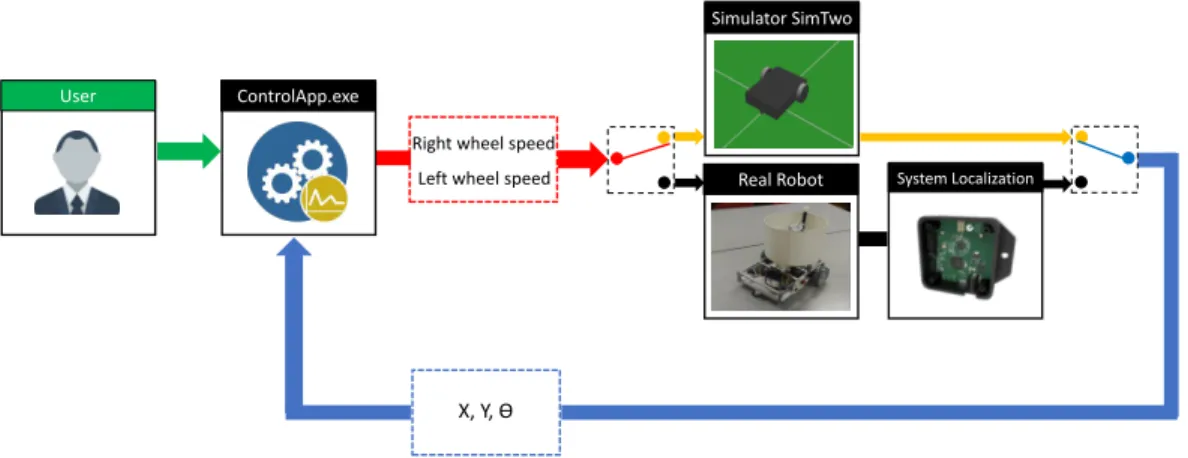
This chapter will describe the software and hardware components used in the proposed approach to perform the scan in an environment with the presence of radioactive or toxic substances. The Figure 3.1 presents the proposed structure and its data ﬂow. The system consists of four main blocks: ControlApp, Real Robot, System Localization and SimTwo Simulator. This system has easy switching between the real environment and the simulation environment, since it share the same communication protocol.

ControlApp.exe

Right wheel speed

Left wheel speed

X, Y, Ɵ

User

Real Robot Simulator SimTwo

System Localization

Figure 3.1: System architecture proposed for the interaction between the user and the robot.

The real robot used in this work was previously made by the supervisors for other projects that encompass mobile robotics.

(54)

3.1 ControlApp and Communication

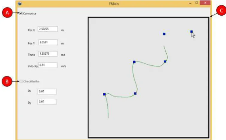
ControlApp is a graphical application for remote access to the robot, developed in the Lazarus programming platform. ControlApp deals with real and simulation environment. This consists of an interface between man and the robot developed for the user to be able to obtain information related to the simulation and real environment such as, speed, position and orientation of the robot in real time. The Figure 3.2 presents the developed interface. The highlighted points A, B and C will be explained below.

Figure 3.2: Interface between ControlApp and the user, highlighting its functionalities: A - Communication, B - Inserting Waypoints and C - Robot navigation area.

Point A displays the checkbox that enables and disables communication between Con-trolApp and real or simulated WMR. The communication protocol used is User Datagram Protocol (UDP) (More information about this protocol can be found in [59]). Each de-vice (real robot, simulated robot and App control) has an IP to be identiﬁed. A packet encoding the robot position, orientation and distance sensor data is sent from robot to ControlApp, whereas a packet containing the right and left speed wheels is sent from ControlApp to robot.

(55)

3.1. CONTROLAPP AND COMMUNICATION 33

created through the valuesDxandDyinserted by the user, which represents the distance between waypoints in x and y. An example of a connectivity grid can be seen in Figure 3.3, where the environment has a dimension of 4 meters long by 4 meters wide and the waypoints are equidistant 0.67 meters each other.

Figure 3.3: Connectivity grid where resolution of the grid is deﬁned by the user.

Point C shows the robot’s navigation area bounded by the existing square. The inner area of the square can be replaced by the 2D plant or even an top view image of envi-ronment that the robot will scan. The route that the robot executes is presented by the green line which is updated in real time.

Other relevant functionalities of the ControlApp are not presented in the interface are the calculations of the wheel speed control of the robot, the robot’s path planning and the calculation of the trajectory. Note that this software runs on a computer external to the robot.

Communication Between ControlApp and Real Robot or Simulated Robot

Due the ControlApp runs on a computer external to the robot, it is necessary to implement a way of communication that allows the transfer of data. As will be discussed in section 3.2 the robot has integrated Wi-Fi, which makes it possible to establish a communications network between ControlApp and Robot.

(56)

types of data in two modes, loopback network for tests in simulation, and in a Wi-Fi network, for implementation in the robot prototype.

The adopted network protocol was UDP. Although it does not guarantee the reception of the data, in contrast to the Transmission Control Protocol (TCP) protocol that allows reception with reliability, which makes TCP slow, the UDP has high speed [60]. In this way, ControlApp must previously know the IP address of the robot that is connected in the same network, besides the port available for the communication and its identiﬁcation establishing a system UDP/IP as described in Figure 3.4a where the communication port is 9808. Tests and simulations occur in a loopback network as shown in Figure 3.4b.

Raspberry Pi 3 192.168.0.1: 9808

192.168.0.2: 9808

(a) Real robot.

Localhost

UDP/IP 127.0.0.1:9808

(b) Simulated robot.

Figure 3.4: Communication between robot and ControlApp.

3.2 Real Robot Description

(57)

3.2. REAL ROBOT DESCRIPTION 35

robot.

Figure 3.5: Prototype of real mobile robot.

3.2.1 Structural Constitution of the Robot

The WMR is designed to perform the scan moving in a plane environment. Its supporting structure is entirely composed of aluminum extrusion proﬁle in X, as shown in Figure 3.6. This material was selected because of its high mechanical strength, its rigidity and its lightness, thus providing robustness and durability to the mobile robot. At the top, the robot has an object with a circumference of 25 cm in diameter, which has utility for the ground truth system of location that will be described later in this work in subsection 3.4.3.

Figure 3.6: Detail of the support structure of the robot built with aluminum extrusion proﬁle in X.

(58)

degrees of freedom; [x, y, θ]T_{. The prototype has three wheels, two of which are coupled to}

independently stepper motors. The other is castor wheel which has the support function. This model of WMR is widely used because of the simplicity of construction and control [61].

The Table 3.1 presents the dimensions of the mobile robot structure:

Table 3.1: Dimensions of real WMR

Robot Description Dimension Unit

Width 0.28 m

Length 0.35 m

Wheel diameter 0.1 m

Wheel thickness 0.025 m

Robot mass 3.4 Kg

3.2.2 Kinematic Model of Differential Robot

According to Roland Siegwart “Kinematics is the most basic study of how mechanical systems behave. In mobile robotics, we need to understand the mechanical behavior of the robot both in order to design appropriate mobile robots for tasks and to understand how to create control software for an instance of mobile robot hardware” [4].

This subsection will be dedicated to present the mathematical notation that represents the kinematics involving the robot based on the literature in the area [4], [20]. It will be described how the movement of a diﬀerential robot occurs. For a better understanding, the kinematic model will be divided into three parts: pose, linear and angular velocity and the last part will present the non-holonomic constraint model.

Pose

The WMR has three degrees of freedom, and its pose in the 2D plane is deﬁned by the state vector in a global coordinate frame (Xg, Yg). That deﬁne an arbitrary inertial basis

(59)

3.2. REAL ROBOT DESCRIPTION 37 Xr Xg P Ɵ Yg x y 0 b w Yr Vl Vr V

Figure 3.7: Robot in the plane representing the global robot reference frame.

ξg =

x(t) y(t) θ(t)

T

(3.1)

The robot frame is in motion attached to the robot (Xr, Yr) . The relation between

the global and robot frame is deﬁned by the rotation matrixR(θ(t)) as show equation 3.2 and 3.3.

R(θ(t)) =

      

cos(θ(t)) sen(θ(t)) 0 −sen(θ(t)) cos(θ(t)) 0

0 0 1

       (3.2)

ξr =R(θ(t))·ξg (3.3)

Linear and Angular Velocity

The velocity of each wheel is controlled by a step motor. Deriving the state of the robot in the global reference frame, the speed relation is obtained as shown in the equation 3.4:

˙

ξg =

˙

x(t) y˙(t) θ(˙t)

=       

cos(θ(t)) 0

sen(θ(t)) 0

0 1        ·  

V(t)

w(t)

 

(60)

The input variables of this system are linear V and angular w velocities of the robot, obtained by the wheel speeds as shown by equations 3.5 and 3.6:

V(t) = Vr(t) +Vl(t)

2 (3.5)

w(t) = Vr(t)−Vl(t)

b (3.6)

Where b is a constant that represents the distance between the traction wheels of the robot at its point of contact with the ground.

Non-Holonomic Restriction

For any state [x(t), y(t), θ(t)]T _{of the robot, the motion must respect the constraint}

im-posed by the equation 3.7 preventing sideways slippage, i.e, avoid movements perpendic-ular to the axis of the robot’s linear velocity as shown in 3.8 in case of a lateral parking attempt.

˙

y(t)·cos(θ(t)) = ˙x(t)·sen(θ(t)) (3.7)

Xg Yg

Xr P

Yr

Vl

Vr V

(61)

3.2.3 Electronic Hardware

The mobile robot, in which the practical tests were carried out, has an elaborate electronic structure to move through the room independently. For that, the WMR has embedded on its base some electronic components, battery, sensors, Raspberry computes and Arduino shields. In this section will present these components. It will not address detailed working concepts of the components, because it is out of the main scope of work. The block diagram of Figure 3.9 shows the high-level component block. Note that the electronic architecture on the robot is arranged which has been designed to be compact to ﬁt over the structure and with low consumption for battery operation.

Raspberry Pi 3 Model B

Sensor Geiger (Not used) Arduino Uno (2) Battery Management and Conversor DC/DC Stepper Motor UWB POZYX Tag Drive Stepper Motor Drive Battery 12V Arduino Uno (1) 5V 12V RS232 R S23 2

Figure 3.9: Mobile robot electronic architecture.

The following subsections will be devoted to the description of the components that compose the robot.

Raspberry Pi 3 Model B - The Robot’s Brain

(62)

Figure 3.10: Raspberry Pi model B.

The microcomputer is powered by a step-down DC/DC converter which has a 12V battery voltage input and provides a 5V to Raspberry Pi. The operating system used is raspbian. The microcomputer run an application that is responsible for performing Kalman Filter calculations, communicating with the ControlApp over Wi-Fi and commu-nicating with two Arduinos via USB (emulated serial port). It is responsible for processing the localization data of the Pozyx sensor obtained through the Arduino (2). It also sends and receives data to the Arduino (1) which matches the speed motors and voltage and current of the battery.

Arduino Uno (1) and (2)

The Arduino Uno (see Figure 3.11) is a development board that features an 8-bit AT-mega328 microcontroller with a 5V operating voltage. It has 14 analog ports and 6 digital ports. Its clock capacity is 16 MHz and its ﬂash memory has 32 KB. The real robot has in its architecture two Arduinos Uno, due to its ease of programming and wide connectivity with diverse shields.

(63)

Figure 3.11: Arduino Uno.

Arduino (2) is directly connected to the Ultra-wideband (UWB) Pozyx tag, as shown in Figure 3.12. Thus the development board together with the Pozyx tag receive the data from the four Pozyx anchors scattered around the environment where the robot will scan by calculating the location (x, y) of the robot. More details about the operation of Pozyx will be presented in subsection 3.4.1.

Figure 3.12: Connection between Pozyx tag and Arduino (adapted from [62]).

(64)

Drive and Step Motor

The robot uses two NEMA 17HS16 step motors. Each coupled to one of the traction wheels. Each step of the motor has a resolution of 1.8 degree providing considerable precision for the odometer calculations.

It uses a CNC shield V3 as interface between the Arduino and two Allegro MicroSys-tems drivers - A4989, each one responsible for one motor. In this way the stepper motor receives a sequence of logical levels of voltage that will feed its coil, where it will pass current, resulting in an electromechanical transformation, moving the wheels of the robot. Figure 3.13 shows how the Arduino is coupled together with shield CNC V3 and Allegro MicoSystem chip a4989.

Figure 3.13: Connection between Arduino, CNC shild V3 and chip Allegro MicroSystems A4989.

UWB Pozyx Tag

(65)

According to the manufacturer, the Pozyx tag is an Arduino compatible shield that provides accurate positioning and motion information. The Pozyx tag connects to an Arduino board using long wire-wrap headers which extend through the shield. This keeps the pin layout intact and allows another shield to be stacked on top [62], as shown the Figure 3.14.

Figure 3.14: Interface of Pozyx system tag to connect at Arduino [62].

3.2.4 Robot Software

The robot sofware is an application developed in Lazarus which is responsible for various operations, such as localization and movement. This application runs on the Raspberry Pi integrated into the robot and manages communications with Arduino (1) and (2) as well as ControlApp. The ﬂow of the operations performed by the application was modeled by a petri net to represent the system in a discrete mode conduct by events which can be veriﬁed in Appendix B.

(66)

3.3 Description of the Simulation Model

To test the algorithms and methodology used to perform the scan of an environment with a mobile robot was used the SimTwo Simulator [63]. According to its own developer Paulo Costa, the SimTwo is “a realistic simulation system that can support several types of robots. Its main purpose is the simulation of mobile robots that can have wheels or legs, although industrial robots, conveyor belts and lighter-than-air vehicles can also be deﬁned” [64]. By using this simulator it was possible to validate the approach in a 3D virtual environment before performing the tests for practical validation. Figure 3.15 displays the workspace of this tool. This section will preset the model performed for the simulation describing the simulated robot, the scenario and method used to insert the uncertainty in the Pozyx system. Further details of the functions and tools of the simulator can be found in [64], [65].

Figure 3.15: Overview of SimTwo simulator tabs and tools [64].

(67)

3.3. DESCRIPTION OF THE SIMULATION MODEL 45

to handle the equations directly [66]. The structure of the simulated robot is deﬁned using boxes, cylinders and joints (connections between bodies and wheels), which are arranged to form a structure similar to that of the real robot, as can be seen in Figure 3.16.

Figure 3.16: Simulated robot.

The simulator has a tab named “code editor” which represents the Integrated Devel-opment Environment (IDE) where a Pascal-based code is implemented, referring to the actions that the robot will perform inside the simulator, i.e. its control parameters [66]. In this tab it is also implemented the communication UDP/IP between the simulator and ControlApp already presented in section 3.2. The WMR exact pose (x, y, θ) in simulation environment is easily obtained with an existing function in the simulator. On the other hand, real localization system are subject to errors and uncertainties due to the real sen-sors. Previous work [67] addressed the estimation for the pose of the real robot using the Kalman ﬁlter to perform the fusion between the odometry and the UWB-ToF sensor. It also outputs the model of the covariance matrix errors for the positioning (equations 3.8, 3.9 and 3.10).

xerror =−0.074 (3.8)

yerror =−0.013 (3.9)

R =

 

0.0015 0.0002

0.0002 0.0005

 

 (3.10)

The values obtained in xerror and yerror provide the average of the errors in relation

(68)

estimation of the location of the robot in the simulator. The θ component of the robot pose is not inﬂuenced by noise in the simulation, due to the fact that the Pozyx sensor does not provide this component, only xand y.

3.4 Structure and Operation of Localization

Hard-ware

In this section will describe the hardware used in the approach proposed for the low cost indoor location to WMR. Currently systems based on artiﬁcial vision with cameras have high-accuracy. However, these high-accuracy systems have a high price disadvantage, which can cost more than a thousand euros. Another disadvantage is the blind spots and the inﬂuence of the luminosity that can change in the environment. Due to these negative points an alternative approach to locating a mobile robot was adopted.

Various methods can be found for the location of the mobile robot, such as Radio Frequency (RF) technologies that are widely diﬀused because of their relatively low cost in addition to the low processing power required. Two approaches are well accepted by the academic community for localization using RF, which are: (i)The technique Received Signal Strength (RSS) which measures the distance between the sender and the receiver using signal power received at the receiver. (i) The technique Time of Flight (ToF) measures the diﬀerence between the instant of time at which the signal is transmitted and the time of arrival at the receiver. With the interval of time and the speed of wave propagation in the environment, the distance between the transmitter and the receiver is obtained.

Application of a Mobile Robot to Spatial Mapping of Radioactive Substances in Indoor Environment

Application of a Mobile Robot to

Spatial Mapping of Radioactive

Substances in Indoor Environment

Luis Fernando Piardi

Application of a Mobile Robot to

Spatial Mapping of Radioactive

Substances in Indoor Environment

Luis Fernando Piardi

Acknowledgement

Abstract

Resumo

Contents

List of Tables

List of Figures

Acronyms

Chapter 1

Introduction

1.1

Motivation and Framework

1.2

Objectives

1.3

Document Structure

Chapter 2

Related Work

2.1

Wheeled Mobile Robot Applied in Monitoring

and Surveillance

2.1.1

Quince Robot

2.1.2

SIAR Robot

2.1.3

SACI Robot

2.1.4

Soryu Robot

2.1.5

Roomba Robot

2.1.6

Curiosity Robot

2.2

Locomotion of Wheeled Mobile Robots

2.2.1

Ackerman Steering Geometry

2.2.2

Omnidirectional Geometry

2.2.3

Differential Geometry

2.3

Localization and Navigation

2.3.1

System Based on Wire Guidance

2.3.2

Systems Based on Strip Guidance.

2.3.3

Systems Based on Marker

2.3.4

Systems Based on Trilateration and Triangulation

2.3.5

Perfect Match

2.4

Path Planning

2.4.1

Roadmap

2.4.2

Cell Decomposition

2.4.3

Sampling-Based Path Planning

2.4.4

Potential Field

2.4.5

A* Algorithm

2.4.6

Genetic Algorithm

2.5

Travelling Salesman Problem

A

B

C

**A* Algorithm**