Trajectory Planning of Mobile robot in Unstructured Environment for Multiple Objects

(1)

Environment for Multiple Objects

MUHAMMAD ARSHAD*, AND MOHAMMAD AHMAD CHOUDHRY**

RECEIVED ON 05.03.2009 ACCEPTED ON 18.11.2009

ABSTRACT

In this paper we have presented a novel technique for the navigation and path formulation of wheeled mobile robot. In a given environment having obstacles, a path is generated from the given initial and final position of the robot. Based on the global knowledge of the environment a global path is formulated initially. This global path considers all the known obstacles in the environment and must avoid collision with these obstacles, i.e. the formulated path must be safe (collision free). For global path formulation strategic schemes have been employed using the a priori knowledge of the environment. The global path is fed to the robot. When unknown obstacles come in the path of the robot, it must deviate from the given global path and should generate a local path to avoid collision with the new unknown obstacle. By using sensors data the reactive schemes have been implemented for local path formulation. For local path formulation the path has been subdivided into intermediate steps known as sub goals. In the existing approaches known and unknown objects are considered separately. But in some of the practical applications known and unknown objects need to be considered simultaneously. This paper considers the problem of robot motion formulation in an environment having already known obstacles and unknown new moving objects. A Novel algorithm has been developed which incorporates local path planner, optimization and navigation modules. As unknown objects can appear in the environment randomly therefore uncertainty in the environment has been considered.

Key Words: Global Path Planner, Local Path Formulation, Unknown Environment, Different Objects, Collision Detection.

* Ph.D. Scholar, and ** Professor,

Department of Electrical Engineering, University of Engineering & Technology, Taxila.

1. INTRODUCTION

both the robot manipulators as well as for mobile robots. But due to their free movements in the environment the mobile robots have greater chances to face obstacles in their path. Therefore, obstacle avoidance becomes a key issue in mobile robots motion planning. So it is very important that wheeled mobile robots have the intelligence and appropriate capabilities for motion planning and control schemes. It has a number of challenging issues. The most important is the environment in which the robot

(2)

Mehran University Research Journal of Engineering & Technology, Volume 31, No. 1, January, 2012 [ISSN 0254-7821]

has to carry out tasks. Mobile robot motion in an obstacles environment can be exemplified as to start from an initial point 1 and goes to the final point 2 avoiding obstacles. An algorithm for collision avoidance has to generate and test paradigm [1]. An easy method is to find a straight line path from point 1 to point 2. This path has to be tested for the collision of the robot with the obstacles. If collision is detected through range sensors it should modify its path to avoid collision with the obstacles. In case of collision detection a new path has to be generated locally. This process is continued until there in no collision detected. This problem can be solved in a three level process. First level is the specification level in which the robot obstacle free configuration space is partitioned into many cells. The relation between adjacent cells is determined and is represented in the form of graph. Any path formed by connecting cell containing point 1 to the cell having point 2 and avoiding obstacles satisfies the specification. Second is the execution level, in which the length of the chosen path is reduced by using optimization techniques. Third level of the process is the implementation level. In this phase the optimized path is converted into time based trajectory to be fed to the controller. A reference trajectory is generated traversing the sequence of cells given by the path. Robot controllers are constructed such that the reference trajectory is followed. The symbolic approach has been presented in [2]. In symbolic approach a framework has been described to provide the knowledge of what has been done and what is to be done. The aim of symbolic control is to enable the usage of methods of formal logic, language and automata theory for solving effectively complex planning problems for robots and teams of robots. The limitation of symbolic approach is that the search performed at the execution level is involved more than the path finding and this is related to the classical problem of model checking in formal analysis.

For motion planning different techniques have been developed by Koditschek, et. al. [3] and Borenstein, et. al. [4], considering the geometrical constraints. They include potential field approach and vector field histogram

(3)

the same results as planning with A* for each new piece of information, but is much faster. The reason is that D* adjusts optimal path costs by increasing and lowering the costs only locally and incrementally as needed. Instead of a regular grid, Quadtrees can be used to reduce memory requirements. So a modified data structure can be used in which cells of the highest resolution may be added around the perimeter of each quadtree region. The drawback of framed-quadtrees is that they can require more memory than regular-grids in highly cluttered environments because of the overhead involved in the book-keeping.

2. CONFIGURATION OF WHEELED

MOBILE ROBOT SYSTEM

The robotic system that we have used is a three wheels mobile robot. It is a non-holonomic system. It has a differential drive system. This robot is very useful in the real world environments testing. The two rear wheels are driven by dc motors separately. Fig. 1 shows the wheeled mobile robot platform.

2.1 Model Constraints

Wheeled mobile robots have mechanical devices, have electromechanical elements embedded controllers and digital circuits. Therefore they are very complex systems. These robots operate in unstructured environment. Due to various constraints and complexity robot motion

planning and control is challenging for developing a computationally efficient framework. The platform that we have used is a nonholonomic system. It has nonholonomy constraints which involve equations having the time derivatives of the system configuration variables. These equations are Non-integrable and they arise when the system has fewer controls than configuration variables. For example a car-like robot has two controls i.e. linear and angular velocities, while it moves in a 3-dimensional configuration space. Any path in the configuration space does not necessarily correspond to a feasible path for the system [6]. That is why the purely geometric techniques developed in motion planning for holonomic systems do not apply directly to nonholonomic ones [7]. While the constraints due to the obstacles are expressed directly in the manifold of configurations, nonholonomic constraints deal with the tangent space. Nonholonomic motion planning itself is a difficult task even in the absence of obstacles. There is not any general algorithm to plan motions for any nonholonomic system such that the system is guaranteed to reach exactly to a given goal [8]. Existing results are for approximate methods in which the system reaches approximately to the goal. Exact methods have been used for special classes of systems. Obstacle avoidance adds another level of difficulty in which we should take into account both the constraints due to the obstacles (configuration parameters of the system) and the nonholonomic constraints which link the parameter derivatives. Geometric techniques for obstacle avoidance should be combined with the control theory for nonholonomic motions.

2.2 Path Planning

Mobile robots research can broadly be classified into

three different categories. These categories are position

estimation, path planning and driving control. The Path planning considers the geometrical concerns of mobile robot motion without accounting the time element. It

searches for a set of collision-free path nodes that leads

the mobile robot from the initial point to the target

(4)

position. Path planning problem is solved in two steps. In the first step a collision free path is formulated. If it is

decided that a collision free (safe) path exists then this

path is fed to be executed by the robot. So in the second step the formulated safe path is converted into

executable form. For mobile robots path planning approaches can broadly be classified into two

categories. One uses exact representations of the environment while the other uses a discretized

representation. Advantage of discretization is that in this representation the computational complexity of path

planning can be controlled by adjusting cell size. While in exact methods, the computational complexity is a

function of the number of obstacles which is normally

not controllable. Normally motion planning problems are solved by approximated algorithms. Exact solutions

exist but only some special small time controllable systems can be solved by exact solutions.

3. MOBILE ROBOTS KINEMATICS

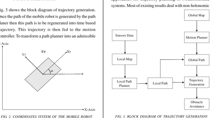
We have developed the kinematics model for our mobile robot and is presented in this paper. Kinematics model of wheeled mobile robot can be obtained with a differential geometric point of view by considering rolling without slipping. The motion planner generates a geometrical path free of collisions, but the motion controller needs the time based trajectory as the input. Therefore, it is necessary that before giving it as input to the controller this geometrical path must be converted into time based trajectory. The geometrical collision-free path in this research has been assumed to be a sequence of points in three dimensions. These are x, y and θ. For the trajectory function parametric cubic spline function in the following form has been used.

x=x (t), y=y (t), θ= (θ)

The parametric cubic spline function is as given:

x(t) = a_1xt3_{+ a} 2xt

2_{+ a} 3xt + a4x

y(t) = a_1yt3_{+ a} 2yt

2_{+ a} 3yt + a4y

θ(t) = a₁_θt3_{+ a} 3θt

2_{+ a} 3θt + a4θ

Boundary Conditions: In our case there are two boundary

conditions relating to the position and velocity of the

robot respectively. The mobile robot has to start from its

initial position and must reach its destination or goal point. This is the first boundary condition which must be satisfied.

Mathematically:

X_init = X (t=0) and X_fin = X (t=T)

The second boundary condition is that initial and final velocity of the mobile robot must be zero. i.e.

0 ) ( . ) 0 ( . = = =

= X t T

t X

To transform the reference cartesian system from global axis to local axis the following transformation matrix has been used.

( )

⎥

⎦

⎤

⎢

⎣

⎡

− = 1 0 0 0 cos sin 0 sin cos θ θ θ θ θ R

The non-holonomic constraints are:

θ θ sin . sin . y x =

The developed control system is as:

2 1 0 0 0 1 1 0 0 0 0 sin sin cos cos cos . . . . v v v v v y x

⎥

⎦

⎤

⎢

⎣

⎡

⎥

⎦

⎤

⎢

⎣

⎡

⎥

⎦

⎤

⎢

⎣

⎡

⎥

⎦

⎤

⎢

⎣

⎡

+ + = ω θ ω θ ω ω θ

(5)

The above developed model is transformed into chained form as:

1 3 . 4 1 2 . 3 , 2 . 2 , 1 .

1 vc z vc z z vc z z vc

z = = = =

Where ν_c1 = νcosω and ν_c2 = νsinω

Obstacle avoidance is very important while the speed of robot and position of the front wheel is not important. Therefore, the control system is simplified as:

ω ω

θ θ

θ

sin 0 0 cos 0 sin cos

. . .

v l v

y x

⎥

⎦

⎤

⎢

⎣

⎡

⎥

⎦

⎤

⎢

⎣

⎡

⎥

⎦

⎤

⎢

⎣

⎡

+ =

In the aboveequation , l is the distance between the axles of front and rear wheels; V is speed of the robot and ω is the steering angle.

4. GENERATION OF TRAJECTORY

FROM THE PATH

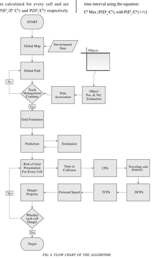
Fig. 3 shows the block diagram of trajectory generation. Once the path of the mobile robot is generated by the path planer then this path is to be regenerated into time based trajectory. This trajectory is then fed to the motion controller. To transform a path planner into an admissible

trajectory is a typical problem in the field of robotics. This problem has been investigated in literature mainly considering the manipulators. There are various approaches which address geometric constraints of obstacle avoidance and the Kino dynamics. These techniques explore the phase space using discretization and graph search methods. These types of algorithms provide approximated solutions and are time consuming. Only few of them deal with obstacle avoidance for Nonholonomic mobile robots. Trajectory planning for a mobile robot has to execute optimal path from the given initial position to the target position [9]. If the obstacles are not considered even then computing admissible path for nonholonomic mobile robot between two configurations is a difficult task. There is no algorithm which guarantees nonholonomic mobile robot system to reach its goal exactly. If our wheel mobile robot has to move from its initial location (0,0,0) to the target location (x,y,θ), it has to perform a pure rotational motion to the location (0,0, atany/x). Then it will perform a translational motion to the location (x,y, atan y/x) and then a rotational motion for steering to the target location. There are several approaches for trajectory planning of Nonholonomic systems. Most of existing results deal with non-holonomic

FIG. 2. COORDINATES SYSTEM OF THE MOBILE ROBOT

Motion Planner Global Map

Global Path

Local Path

Planner Local Path

Obstacle Avoidance Trajectory Generation Local Map

Sensors Data

(6)

systems and object avoidance in two ways. One is to focus on motion planning ignoring obstacles. The other is to modify results from a holonomic planner. The approach of approximating a holonomic path into a sequence of admissible collision free paths has two steps. In the first step if a solution for the path exists then with geometric path planner a collision free path is planned. In the second step the path is subdivided into sub paths. These sub paths are joined together to form a collision free path. It is necessary that a collision free path has been calculated geometrically ignoring the kinematics constraints for applying the above technique and a geometric routine must satisfy that the path is collision free. The steering method consists of the shortest admissible path. Steering methods give the sequence of admissible paths whose length is related with the first collision free path. When the path is closer to the obstacle it should be further subdivided. From the optimal trajectory planning a path is provided to mobile robot having shortest distance, minimum driving time and minimal tracking error. An admissible trajectory of a robot is the solution of differential system corresponding to the kinematics model of the mobile robot with the given initial and final conditions. A path is the image of a trajectory in configuration space. A trajectory in the sequel is a continuous function from some real interval [0,T] in configuration space. For nonholonomic motion planning the objective is to find collision-free admissible paths for mobile robot in the configuration space. Block diagram for trajectory generation of mobile robot is shown in Figure 3. Motion planners compute paths which have to be transformed into trajectories. Transformation of the path into a trajectory should be elaborated by simplifying the kinematics model of the robot. The path must be smoothed before computing the trajectory.

5. PROBLEM FORMULATION OF

MOBILE ROBOT

The Mobile robot has to move from initial position {X_init=(x_j,y_i; θ_i)T_{} to the given target (final position)}

{X_fin=(x_f, y_f, θ_f)T_{}. The problem is to find the trajectory}

X(t)=[x(t), y(t), θ(t)]T_{and the traveling time T. There are}

(7)

5.1 Static Path Planning

In this case the robot has to move among static or fixed obstacles therefore it is constrained by its geometry and workspace. There are three main categories. One is the Exact Method in which an exact representation is computed for the free configuration space. If an admissible trajectory exists then these methods guarantee its solution. Trajectory is generated by combining the sub trajectories obtained by connecting the initial and final configurations. The main problem in these methods is the representation of the space. The representation can be done in three different ways, i.e. Roadmap, cell decomposition and boundary representation [11]. Second category is Approximate Method which is used in problem where the precision of exact method is not involved. In these techniques the free space representation is approximated thus reducing the planning time. These methods are further categorized into artificial potential field methods and approximate cell decomposition methods. Artificial potential methods are used for real time obstacle avoidance of robot. In this method the obstacle is considered as a source of repelling for robot and the target acts as attraction force. This method is simple. It does not need exact representation of free configuration space thus planning is fast. But the problem in this method is that local minimum exists in the potential field. In approximate cell decomposition method the space is divided into three types of cells. They are called full, Empty and mixed. Full cells are those which lie entirely in the configuration space of the obstacles. Empty cells lie in the free configuration space. The rest of the cells are called mixed. The main problem of this method is the limitation of the number of DOF (Degrees of Freedom). Another problem is the full representation of motion constraints. The third category is the Hybrid Method. Hybrid method is the combination of several methods. Hybrid methods include Mixed methods and Task managers. Mixed method is the combination of artificial potential method and approximate cell decomposition method [12]. Task manager [13] uses two

or more basic planners, in which one is fast and uses heuristic while the other is complete but is slow.

5.2 Velocity Planning

In this case the mobile robot has to move among dynamic obstacles. We have to determine the relative velocity of the robot and the moving obstacles so that there is no collision. To do this complete information (future trajectories), is require and its solution is not guaranteed. Velocity planning can be done for objects that are moving with uniform velocities, using the velocity obstacle concept [14]. Collision is avoided if robot velocity is chosen such that its velocity relative to obstacles velocity does not enter the corresponding collision cones. For dynamic obstacles correct environment sensing is required to estimate its proper position and velocity. For appropriate decisions proper sensing representation is needed to collect sensor data of the critical object in the environment of the mobile robot, which helps in the estimation of the position and velocities of the objects in the environment of the mobile robot. Main problem is data association, which decides the correspondence of the new data with the existing track. Track management decides that either new track should be created or the old one must be maintained.

6. THE DEVELOPED TECHNIQUE

(8)

that moving object is lost due to occlusion problem. Therefore, uncertainty in the environment estimation has been taken into account by the probabilistic reasoning technique. Risk of the Probabilistic grid representation has been estimated for each cell using sensor data. A four dimensional grid is formed to encounter the position and velocities of the object relative to our wheel mobile robot. At each time interval occupancy grid is estimated by combining the estimation step and prediction step. Bayesian Formulation has been used for static Estimation. Probability distribution is given as:

( )

= ∑ = ×∑FPr SFK K

r P

SFK F rP k

s r

p 1 ( )

) ( ) ( / α

In the above equation, S is a searched variable, K is a known variable and F is a free variable, α is a normalization term. Probability occupancy of each cell of the grid is estimated by the sensor data (false alarm for detecting non-existing objects and missed detection when existing object is not detected) as:

∑ = ∏= = = Π = ⎟ ⎟ ⎠ ⎞ ⎜ ⎜ ⎝ ⎛ ⎟ ⎟ ⎠ ⎞ ⎜ ⎜ ⎝ ⎛ ⎟ ⎟ ⎠ ⎞ ⎜ ⎜ ⎝ ⎛ ⎥⎦ ⎤ ⎢⎣ ⎡ s M s

s M_CCM

s Z r P C C E r P M C CE s Z r P s s M r P C C E r P C r P M C CE r P 1 1 ) / ( 1 ) ( ) / ( ) ( ) ( α ς ζ

In the above equations C represents the cell, E_C represents state of the cell and ζ is observation set. Z_s is one observation and is four dimensional. S is the number of observation and M is a matching variable. Estimation in

changing environments has been taken into account by the history of sensory observations. Prediction and Estimation have been used for this estimation. In prediction we estimate occupancy probability at time k of a cell by

k-1 occupancy grid while estimation is based on the previous prediction. They are represented by P_r(Ek

c/C

k _Uk-1_{) and}

P_r(Ek c/Z

k_Ck-1_{) respectively. Where C}k_{represents cell at time}

k and Ek

c represents state of C at time k respectively. Bayes

Filter has been used.

XK_{= f}K_(XK-1_{, U}K-1_{, W}K₎

In the above Bayes filter Xk_{is a state sequence, K}∈_{N of a}

system, fk_{is a nonlinear transition function and U}k-1_{is a}

control variable (speed or velocity) for sensor to estimate ego-movement between time k-1 and k. Wk_{is the process}

noise. When Zk_{is the sensor observation of the system at}

time k, filtering recursively estimate Xk_{from sensor}

measurements:

Z_K = HK_(XK_{, V}K₎

6.1 Avoidance of Collision

For developing technique for the wheeled mobile robot to avoid collision Bayesian Occupancy Filter has been employed. By this the forward speed values of the wheeled mobile robot are selected. These are the values which avoid collision with the moving obstacles. With occupancy property the danger property has also been implemented. Danger property has been estimated in which the probability of each cell of the grid that it is a hazardous is estimated, independently of the occupancy estimation. Time to collision and traveling safe distance are the two

criteria for estimating the danger encountering. Closest point of approach is the relative position of robot and the obstacle and is called safety distance. Time to closest point of approach is the time to reach this safe distance. Distance at this closest point of approach is the distance separating mobile robot and object when closest point of approach has reached. The previous criterion is evaluated for every cell Fig. 4 shows the flow chart of the developed algorithm.

6.2 Application of Collision Avoidance

(9)

obtained by occupancy and danger probabilities. These probabilities are calculated for every cell and are represented by P(Ek

c/Z

k_Ck_{) and P(D}k c/C

k_{) respectively.}

Practically the probable occupied cell is searched at every time interval using the equation:

Ck_{Max {P(D}k c/C

k_{), with P(E}k c/C

k_{) > ½}}

START

Environment Data Global Map

Global Path

Track Management

Continue

Grid Formation

Prediction

Data Association

Object Pos. & Vel. Estimation

Estimation

Risk of Grid Presentation For Every Cell

Time to

Collision CPA Traveling safe distance

DCPA TCPA

Forward Speed Danger

Property

Whether each cell Danger

Target No Yes

Yes

Objects

No

(10)

7. RESULTS

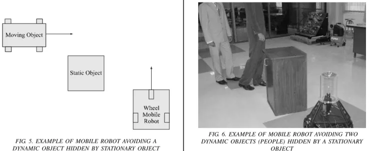
An experimental situation for the collision avoidance for the mobile robot is shown in Figs. 5-6.

Fig. 5 shows the situation when the mobile robot is moving towards its target. There is a stationary object

and a moving object approaching in the path of the mobile robot. The moving object is detected by the mobile robot. For a small period of time the moving object is hidden by

the stationary obstacle. Fig. 7 shows the velocity curve of the mobile robot. It is clear from Fig. 7(a) that the robot gains speed from time t=0 to t=10 seconds. That is, it attains its maximum velocity of 0.5 m/s. Then the moving

object is detected which has the probability to collide with the robot, so velocity of robot decreases. From time t=12 seconds to t=14 seconds the object is hidden by the stationary object. During this time period our technique considers the probability occupied by the

hazardous cell of the grid. Therefore the mobile robot stops till the moving object reappears. Then the robot accelerates at t=14seconds when there is no risk of

collision. Figure 6 shows a practical example of mobile robot moving towards its target. There is a stationary object (rack) and two dynamic obstacles (moving persons) approaching in the path of the mobile robot.

Fig. 7 (b) shows the velocity curve of the mobile robot

FIG. 5. EXAMPLE OF MOBILE ROBOT AVOIDING A DYNAMIC OBJECT HIDDEN BY STATIONARY OBJECT

FIG. 6. EXAMPLE OF MOBILE ROBOT AVOIDING TWO DYNAMIC OBJECTS (PEOPLE) HIDDEN BY A STATIONARY

OBJECT

when there are two moving obstacles. The robot gains its speed when at time t=11 s it detects a moving object which has the probability to collide with it. Then the object hides behind the stationary object. Our technique

considers the probability occupied by the hazardous cell of the grid during this period and the robot decreases its speed till the moving object reappears. Then the robot accelerates when there is no risk of collision. When the

robot attains its speed towards its target point it detects another moving object having the probability of collision. The robot again decelerates as our technique again considers the probability occupied by the hazardous cell

of the grid during this period. When there is no risk of collision the robot attains its acceleration. Fig. 7(c) shows the velocity curve of the mobile robot for two moving objects one just after the other simultaneously. At time

t=11 s a moving person is detected by the robot having the probability of collision. During his movement the person is hidden behind a stationary rack. Our algorithm works during this time by considering the probability

occupied by the hazardous cell of the grid. So the robot decreases its speed till the person reappears. At time t=14 s the mobile robot detects another person approaching in its path, so the robot further decelerates.

(11)

(12)

8. CONCLUSIONS

In this paper we have presented a new technique for the

trajectory planning of wheeled mobile robot. Existing

approaches consider the static and moving objects

separately. Whereas the practical applications require the

consideration of static and moving objects simultaneously.

The problem of robot motion planning was considered in

an environment consisting of both static and moving

objects. When the moving object is hidden behind the

static obstacle our algorithm considers the probability of

the hazardous cell of the grid. The algorithm developed

was tested for multiple objects hidden behind the static

obstacle. This technique works quite well in highly dynamic

environment.

ACKNOWLEDGEMENT

Authors are thankful to HEC (Higher Education Commission of Pakistan), for providing funds in completing this research.

REFERENCES

[1] Kulic, R., and Vukic, Z., "Methodology of Concept

Control Synthesis to Avoid Unmoving and Moving

Obstacles (II)", Intelligent and Robotic Systems,

Volume 45pp. 267-294, 2006.

[2] Georgiev, A., and Allen, P.K., "Localization Methods

for Mobile Robot in Urban Envirenments", IEEE

Transaction on Robotics, Volume 20, No. 5, October,

2004.

[3] Rimmon, E., and Koditschek, D.E., "Exact Robot

Navigation Using Artificial Potential Functions", IEEE

Transaction on Robotic and Automation, Volume 7,

pp. 501-518, 1992

[4] Borenstein, J., and Koren, Y., "The Vector Field

Histogram-Fast Obstacle Avoidance for Mobile Robot",

IEEE Transaction on Robotic and Automation,

Volume 7, pp. 278-288, 1991.

[5] Papadopoulos, E., Papadimitriou, I., and Poulakakis, L.,

"Polynomial-Based Obstacle Avoidance Techniques for

Nonholonomic Mobile Manipulator Systems", Robotics

and Autonomous Systems, Volume 51, pp. 229-47, 2005.

[6] Laumond, J.P., “Robot Motion Planning and Control”,

Springer-Verlag, London, 1998.

[7] Murray, R.M., Li, Z., and Sastry, S.S., “A Mathematical

Introduction to Robotic Manipulation”, CRC Press, Inc.,

Boca Raton, 1994.

[8] Wang, J., Qu, Z., Guo, Y., and Yang, J., "A

Reduced-Order Analytical Solution to Mobile Robot Trajectory

Generation in the Presence of Moving Obstacles",

Proceedings of IEEE International Conference on

Robotics & Automation New Orleans, LA, April, 2004.

[9] Bui, X.N, Sou_Eres, P., Boissonnat, J.D., and Laumond,

J.P., "Shortest Path Synthesis for Dubins Nonholonomic

Robot", IEEE International Conference on Robotics

and Automation, San Diego California, 1994.

[10] Lefebvre, O., Lamiraux, F., Pradalier, C., and Fraichard,

T., "Obstacles Avoidance for Car-Like Robots Integration

and Experimentation on Two Robots", Proceedings of

IEEE International Conference on Robotics and

Automation New Orleans, LA, April, 2004.

[11] Kulic, R., and Vukic, Z., "Methodology of Concept

Control Synthesis to Avoid Unmoving and Moving

Obstacles", Journal of Intelligent and Robotic Systems,

Volume 37, pp. 21-41, 2003.

[12] Faverjo, B., and Tournassound, P., "The Mixed Approach

for Path Motion Planning: Learning Global Strategies

from a Local Planner", Proceedings of International

Joint Conference on Artificial Intelligence, Milan, August,

1987.

[13] Chen, P., "Improving Path Planning with Learning",

Proceedings. of Machine Learning Conference, Aberdeen,

Scotland, 1992.

[14] Wang, J., Qu, Z., Guo, Y., and Yang, J., "A

Reduced-Order Analytical Solution to Mobile Robot Trajectory

Generation in the Presence of Moving Obstacles",

Proceedings of IEEE International Conference on