Stainless Steel Bonded to Concrete: An Experimental Assessment
using the DIC Technique
Hugo Biscaia
1),* , Noel Franco
2), and Carlos Chastre
3)(Received June 17, 2017, Accepted October 24, 2017)
Abstract: The durability performance of stainless steel makes it an interesting alternative for the structural strengthening of reinforced concrete. Like external steel plates or fibre reinforced polymers, stainless steel can be applied using externally bonded reinforcement (EBR) or the near surface mounted (NSM) bonding techniques. In the present work, a set of single-lap shear tests were carried out using the EBR and NSM bonding techniques. The evaluation of the performance of the bonding interfaces was done with the help of the digital image correlation (DIC) technique. The tests showed that the measurements gathered with DIC should be used with caution, since there is noise in the distribution of the slips and only the slips greater than one-tenth of a millimetre were fairly well predicted. For this reason, the slips had to be smoothed out to make it easier to determine the strains in the stainless steel and the bond stress transfer between materials, which helps to determine the bond–slip relationship of the interface. Moreover, the DIC technique allowed to identify all the states developed within the interface through the load–slip responses which were also closely predicted with other monitoring devices. Considering the NSM and the EBR samples with the same bonded lengths, it can be stated that the NSM system has the best performance due to their higher strength, being observed the rupture of the stainless steel in the samples with bond lengths of 200 and 300 mm. Associated with this higher strength, the NSM specimens had an effective bond length of 168 mm which is 71.5% of that obtained for the EBR specimens (235 mm). A trapezoidal and a power functions are the proposed shapes to describe the interfacial bond–slip relationships of the NSM and EBR systems, respectively, where the maximum bond stress in the former system is 1.8 times the maximum bond stress of the latter one.
Keywords:stainless steel, concrete, bond failure, digital image correlation.
1. Introduction
The first studies on the external bonded reinforcement (EBR) technique using steel plates were carried out in the late 1960s in France by L’Hermite and Bresson, who ana-lyzed the steel-epoxy-concrete connection (L’Hermite and Bresson1967; L’Hermite1977). Since then, there have been many studies characterizing the bonding behaviour of strengthening elements using the EBR technique, initially
with steel plates (Ladner 1978, 1983; Jones et al. 1980; Swamy and Jones1980; Chastre Rodrigues 1993; Ta¨ljsten 1997) and more recently with fibre reinforced polymers (FRP) (Blaschko and Zilch1999; De Lorenzis et al. 2000; De Lorenzis and Teng 2007; Lorenzis et al. 2001; Nakaba et al. 2001; Chen et al. 2005; Aiello and Leone 2008; Martinelli et al.2011; Dehghani et al. 2012; Biscaia et al. 2013,2014). As for the near surface mounted (NSM) tech-nique, although there are some references of its use, only at the end of the 1990s did studies on the performance of this technique associated with the use of FRP rods (Blaschko and Zilch1999; De Lorenzis et al.2000) begin to appear.
Therefore, in most of the studies that can be found in the literature (e.g. Xia 2005; Akbar et al. 2010; Smith 2010; Wan2010; Wan et al.2014; Biscaia et al.2016a,b,2017b), the focus is on bonded joints between FRP composites and concrete but recently there have been more studies on both steel (only with EBR technique) and timber structures (with both EBR and NSM techniques). Still, in reinforced concrete (RC) structural strengthening, stainless steel (SS) is a pos-sible alternative to mild steel or FRP composites due to its durability. Compared to mild steel, the durability perfor-mance of SS is higher, but there is no significant difference between them in terms of weight-strength ratio. However, despite its lower weight/strength ratio, stainless steel has ductile behaviour, and good corrosion resistance which are 1)
Fluid and Structures Engineering, Research and Development Unit in Mechanical and Industrial Engineering, Department of Civil Engineering,
Faculdade de Cieˆncias e Tecnologia, Universidade Nova de Lisboa, Caparica, Portugal.
*Corresponding Author; E-mail: [email protected] 2)
Department of Civil Engineering, Faculdade de Cieˆncias e Tecnologia, Universidade Nova de Lisboa, 2829-516 Caparica, Portugal.
3)
Civil Engineering Research and Innovation for Sustainability, Institute of Structural Engineering, Territory and Construction, Department of Civil Engineering, Faculdade de Cieˆncias e Tecnologia, Universidade Nova de Lisboa, Caparica, Portugal. CopyrightThe Author(s) 2018. This article is an open access publication
International Journal of Concrete Structures and Materials DOI 10.1186/s40069-018-0229-8
important and decisive factors in choosing it for strength-ening structures instead of FRP composites. Nevertheless, a significant and common drawback, whatever the bonded materials are, is the premature debonding of the material used in the bonding strengthening technique. Several authors have been studying the premature debonding phenomenon on FRP composites and concrete joints (e.g. Arduini et al. 1997; Neubauer and Rosta´sy 1997; Bizindavyi and Neale 1999; Harmon et al.2003; Smith and Teng2002; Yao et al. 2005; Teng et al.2006; Wu and Yin2003), FRP and timber joints (e.g. Smith2010; Wan2010; Wan et al.2014; Biscaia et al. 2016a, b, 2017), FRP and steel joints (e.g. Xia and Teng 2005; Akbar et al. 2010; Fawzia et al. 2006; Wang et al.2016; Yu et al.2012; Al-Mosawe et al.2015; Fernando et al.2014) or steel and concrete joints (e.g. L’Hermite and Bresson1967; L’Hermite1977; Ladner1978; Ladner1983; Jones et al.1980; Swamy and Jones 1980; Chastre Rodri-gues 1993; Ta¨ljsten1997; Gomes and Appleton 1999; Van Germet1990; Aykac et al. 2013).
Therefore, researchers have studied the debonding phe-nomenon between two bonded materials through different approaches whether they are experimental, analytical, numerical or embracing part or all of these three procedures. Furthermore, the test setup configuration assumed for this kind of study may vary considerably (Wu et al.2002), with the most commonly used configurations being the double-lap pull or push shear tests, the single-double-lap pull tests, the double strap tests or the 3-point bending tests. Independently of the procedure followed, researchers seem to be fairly unanimous that the debonding failure process of a struc-turally bonded joint can be analyzed and predicted through the relationship between the interfacial bond stress and the slip (i.e. the relative displacement between bonded materials).
Unlike FRP composites, stainless steel has a more com-plex constitutive behaviour, which may change or even eliminate conventional ways of finding the bond–slip rela-tionship. Typically, the bond stresses and the slips are experimentally found in the data collected from strain gau-ges that, before the testing of the samples, were bonded on the strengthening material along their bond length. Thus, to determine the bond stresses, it is assumed that the bond stresses developed between two consecutive strain gauges are constant. To determine the slips, it is first assumed that the strains in the concrete are zero and, by integrating the strains with respect to (and along) the bonded length, the slips within the interface can then be calculated. Dai et al. (2005) proposed an alternative procedure, which eliminates the need to use strain gauges. To determine the interfacial bond–slip relationship, they said that knowing only the displacement at the most loaded end of the strengthening material and the load transmitted to that material is enough to obtain the bond–slip relationship. In both cases, a suffi-ciently long bond length should be considered, but the for-mer method makes the process more expensive because it requires the use of several strain gauges that should not be bonded too far away from each other in order to obtain feasible results.
A more recent alternative to obtain the slips developed within a bonded joint is digital image correlation (DIC), which allows the monitoring of an entire surface (Almeida et al.2016) instead of a single point, as conventional strain gauges do. Once again, researchers have been studying the bond between an FRP composite and concrete (e.g. Marti-nelli et al. 2011; Czaderski et al. 2010; Cruzet al. 2016; Ghiassi et al.2013; Zhu et al.2014). The use of commercial DIC techniques is quite expensive but, nowadays, its use became very economical due to the powerful digital cameras currently available on the market, plus the free software that can be easily found on the web (e.g. Wang and Vo 2012; http://www.ncorr.com/; GOM Correlate) to perform the DIC analysis. However, the reliability of these free software for the assessment of the debonding phenomenon between stainless steel and concrete was not demonstrated so far but its use is unlimited and besides that, to start monitoring laboratory structures under loading, only the initial cost of the digital camera and the corresponding free software installed in a laptop, is needed.
Although some work suggests that the DIC technique can be used to determine the interfacial bond–slip relationship of CFRP-to-concrete interfaces (Ghiassi et al.2013; Zhu et al. 2014), the bond stresses are generally smoothed through a mathematical function that predicts the slips or the strain distributions in the FRP composite. This procedure bypasses the difficulties with obtaining a smoothed displacement result from the DIC technique and the slips fluctuate instead (Zhu et al. 2014). Therefore, when it comes to determining the strains and especially the bond stresses in the interface, the fluctuations in the slip distributions are amplified, which increases the error in calculating the interfacial bond–slip relationship. For this reason, a smoothed and previously known function of the slips or strain distributions is used instead of the real ‘‘peaks and valleys’’ obtained from the DIC technique. However, it is important to note that determining the interfacial bond–slip relationships with DIC can only be viable if the results gathered by using the DIC technique can reproduce the same bond–slip relationship accurately enough and on its own, as the results obtained from other means, such as those reached by the two procedures mentioned earlier. Knowing the interfacial bond–slip relationship within the stainless steel and the concrete due to their bonding with an adhesive is important because it will open up the possibility to analyze and study, using an analytical or a numerical approach, the debonding failure between the stainless steel and concrete by means of either a closed-form solution or by an approximation procedure, respectively.
the RC samples as per the Near Surface Technique (NSM). To monitor the strains in the EBR specimens, several strain gauges were used. In order not to affect the bonded area of the NSM specimens, no strain gauges were used in these samples. In both cases, the DIC technique was used and its viability was checked with the EBR specimens only. In some cases, only the most loaded bonded region could be moni-tored with the DIC technique due to the range of the bonded lengths covered in this work (between 50 and 800 mm). Still, throughout the duration of the tests the slips were quite accurate compared with those obtained from the strain gauges and the load–slip response at the stainless steel loa-ded end was sufficiently reproduced using the DIC tech-nique. Moreover, the slip distributions observed with the DIC technique showed similarities to those obtained from the strain gauges, despite some fluctuations, i.e. with higher slips at the SS loaded end and decreasing towards the SS free end. However, as initially suspected, the differences between the strains from the DIC technique and the strain gauges increased throughout. The interfacial bond–slip relationship between the stainless steel and concrete of the EBR speci-men was then determined from the strain gauges bonded on the stainless steel strips. The results obtained from the EBR specimens, allowed a first attempt to be shown to represent and qualitatively identify the bond–slip relationship of the NSM specimens. Nevertheless, it was also found that the NSM specimens and the stainless steel rods performed better due to the rupture of the stainless steel rods when the bonded length was equal to or higher than 200 mm long.
2. Experimental Program
In order to evaluate the Mode II bond transfer between stainless steel (SS) and concrete, an experimental program including two different bonding techniques was idealized. The Externally Bonding Reinforcement (EBR) and the near surface mounted (NSM) techniques were herein considered. Several bond lengths were tested and their influence on the strength of the interface was analyzed. Table1shows all the tests carried out as well as the designation of the specimens given to each one. Additionally, the instrumentation used on each test is also briefly mentioned in Table1.
2.1 Mechanical Properties of the Materials
The specimens used for the present experimental program were taken from RC T-beams previously tested to a 4-point bending test (Franco and Chastre 2016; Chastre et al. 2016, 2017). The regions of the beams with negligible bending moments, i.e. at the vicinities of the supports (pin-rolled), were used and the stainless steel was bonded at the bottom region of the flange of the T-beam with their ends free of any additional mechanical anchorages. This proce-dure ensures that the concrete used was not sufficiently tensioned to develop or even initiate any cracks that could affect the results obtained now from the single-lap shear tests. The strength of the concrete was evaluated at 28 days of age and 3 concrete cubes were subjected to uniaxial
compression until failure accordingly to the standard NP EN 12390-3 (CEN 2003). The results allowed the average maximum compression stress of the concrete to be calcu-lated by fcm=24.1 MPa, which represents, accordingly to
Eurocode 2 (Eurocode 2 (EC2)1992), a C20/25 concrete. The steel reinforcements of the RC T-beams were also tested under uniaxial tension and its mechanical properties are briefly reported in Table2. More details about the tests of the steel reinforcements can be found elsewhere (Franco and Chastre2016; Chastre et al.2017; Chastreet al.2016). The mechanical properties of the stainless steel were also determined from the tensile tests carried out on 7 strips with a cross section of 2095 mm (width9thickness) and from 6 tests on rods with 8 mm diameter, according to the European standard EN ISO 6892-1 (CEN2009). The results obtained from these tests are shown in Table2.
For the bonding of the stainless steel to the concrete, an epoxy resin was used with the commercial designation S&P Resin 220. The mechanical properties of the epoxy resin given by the supplier were herein considered (S&P Resin 220 2016), i.e. compression strength higher than 70 MPa, shear strength higher than 26 MPa, Young modulus higher than 7.1 GPa, bond stress when used with concrete and at 20C higher than 3 MPa and bond stress to steel at 20C
higher than 14 MPa (after 3 days).
The yielding point of the stainless steel strips is not clearly identified due to its constitutive nonlinearities, existing at a low strain level, whereas the constitutive behaviour of the stainless steel rods is elastic–plastic with a yielding point very clear and easy to identify. Therefore, the constitutive behaviour of the stainless steel strips was approximated to the Ramberg–Osgood relationship (Ramberg 1943) in accordance to:
ess¼ rss
Ess
þarss
Ess
rss
r0
n 1
ð1Þ
where a and n are constants obtained from experimental tensile test of the stainless steel strip andr0is the axial stress in the stainless steel at 0.2% strain. Hence, in the present study, the values determined for a and n are 0.05 and 9.7, respectively. Figure1 shows the stress–strain relationships of the stainless steel in strips and rods obtained from the simple tensile tests carried out in a universal tensile machine with a capacity of 100 kN.
2.2 Geometry and Preparation of the Specimens
form to the flange. The flange was 405 mm wide and the web measured 150 mm wide. The stainless steel was always bonded along the mid line that equally divides the flange in half. For the EBR system, the concrete surface was pre-treated with grinder, whereas for the NSM system, a small groove with 12 mm deep was made in the concrete surface in order to insert the stainless steel rod. The stainless steel strips and rods were all pre-treated with wire brush and then cleaned with compressed air and acetone before starting to bond the SS to the concrete in order to remove contaminants on the surface of the stainless steel (e.g. oil, grease, water, etc.) (Fernando et al.2013).
The EBR system was completed when the epoxy resin was placed on the concrete surface along the bond length and the stainless steel positioned on the resin. For the NSM system,
Table 1 Single-lap shear tests.
Specimen Bond length,Lb(mm) Strengthening technique Instrumentation
SS-EBR-L50 50 EBR 2 LVDTa, 3 SGb, 1 DCc
SS-EBR-L100a 100 EBR 2 LVDTa, 4 SGb, 1 DCc
SS-EBR-L100b 100 EBR 2 LVDTa, 3 SGb, 1 DCc
SS-EBR-L160 160 EBR 2 LVDTa, 5 SGb, 1 DCc
SS-EBR-L240 240 EBR 2 LVDTa, 7 SGb, 1 DCc
SS-EBR-L300 300 EBR 2 LVDTa, 8 SGb, 1 DCc
SS-EBR-L400 400 EBR 2 LVDTa, 11 SGb, 1 DCc
SS-EBR-L560 560 EBR 2 LVDTa, 15 SGb, 1 DCc
SS-EBR-L640 640 EBR 2 LVDTa, 16 SGb, 1 DCc
SS-EBR-L800 800 EBR 2 LVDTa, 21 SGb, 1 DCc
SS-NSM-L35 35 NSM 2 LVDTa, 1 DCc
SS-NSM-L50 50 NSM 2 LVDTa, 1 DCc
SS-NSM-L75 75 NSM 2 LVDTa, 1 DCc
SS-NSM-L100 100 NSM 2 LVDTa, 1 DCc
SS-NSM-L200 200 NSM 2 LVDTa, 1 DCc
SS-NSM-L300 300 NSM 2 LVDTa, 1 DCc
a
Linear variable differential transformer.
b
Strain gauge.
c Digital camera.
Table 2 Mechanical properties of the steel and stainless steel (average values).
Material Section type Yield stress,fy,m(MPa) Ultimate stress,fu,m
(MPa)
Ultimate strain,eu,m
(MPa)
Young modulus,Em
(GPa)
Steel
B 500 SD
/6 538 634 7.5 199
/8 573 675 6.5 212
/12 530 637 11.4 211
Stainless steel
EN 1.4404
2095 260 618 27.2 192
Stainless steel
EN 1.4301
/8 1008 – 9.7 195
the groove was filled with epoxy resin and then the stainless rod was introduced into the groove. These operations were repeated for all the specimens herein considered.
2.3 Measurements and Procedures Followed During the Tests
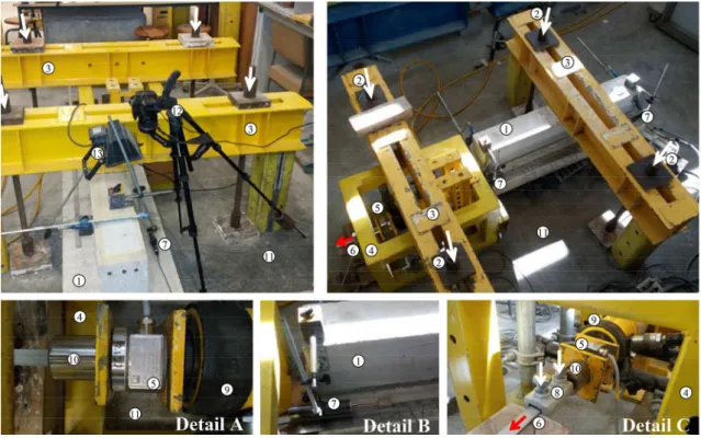
The single-lap shear test was the configuration used in the current work. Figure3shows an overview of the test setup adopted in this study. Actually, this configuration was pre-viously used in the work developed in references (Biscaia et al. 2016a, b, 2017b) for the analysis of carbon fibre reinforced polymers (CFRP) bonded to other structural materials such as concrete, steel and timber allowing the necessary and sufficient experimental data for the evaluation of the bond stress transfer in these joints to be collected. This test apparatus consists of a steel frame where a hydraulic jack is installed. A small steel profile is placed at the rear of the hydraulic jack providing the reaction needed when the SS is pulled out. A pressure cell with a maximum capacity of 200 kN was placed in the front of the hydraulic jack (see Detail A in Fig.3). A mechanical anchorage device con-sisting of a hollow metallic cylinder with two-piece anchor
wedges was installed at the front of the pressure cell (see Details A and C in Fig.3). This device proved not to be sufficient to ensure that the SS would not slip inside the metallic cylinder, between the two anchor wedges, when the hydraulic jack started to push it out. Therefore, another metallic device with two metallic bolts was placed in front of the hollow metallic cylinder. The metallic bolts, when attached, were efficient because they prevented the two-piece anchor wedges from slipping inside the cylinder allowing the loads to be transmitted to the SS-to-concrete interface.
Along the bonded length, several strain gauges TML-FLA-5-17-5L were bonded to the SS strips. Two Linear Variable Displacement Transducers (LVDT), were placed at both edges of the interface. One measured the displacements at the SS loaded end (see Detail B in Fig.3), and the other one measured the displacements at the SS free end. A data logger was used to collect and send all the data to a desktop computer.
Furthermore, a spray paint with a granite speckle effect was used to paint the bonded area of the monitoring area. Figure4 shows the concrete surface before and after
Fig. 2 Scheme of the cross-sectional area of the specimens:adimensions;bEBR system; andcNSM system.
spraying the bonded area to be monitored during the test. A digital camera captured photos with 345695184 pixels at intervals of 5 s during the test. In order to avoid undesired shadows in the pictures, a 100 W artificial spotlight was used. The digital camera was synchronized with the other monitoring devices such as the LVDT and strain gauges. This synchronization allowed the DIC technique to be examined to see if it produces sufficiently accurate results when compared to the monitoring equipment and to test its feasibility for evaluating the debonding process of the SS-to-concrete interface. Therefore, the relative displacements between bonded materials, whether measured by the DIC technique or calculated using the strains gauges, combined with the loads measured through the pressure cell installed at the front of the test setup, allowed the load–slip response to be obtained for stainless steel bonded to concrete, which is a very important relationship for the understanding of the debonding failure process between two bonded materials, e.g. Biscaia et al. 2013a, b, 2016,2017b; Dehghani et al. 2012; Caggiano et al.2012; Carrara et al.2011).
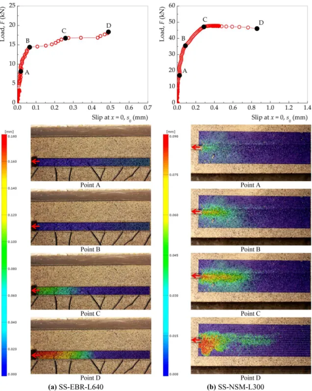
The commercial GOM Correlate software was used to measure the displacements of the painted area. Figure5 shows, as an example, the displacements measured with the GOM Correlate software of specimen SS-EBR-L640 and SS-NSM-L300 at four different stages of the load–slip response obtained from each sample. Figure5clearly shows the range of displacements measured along the bond length, the SS loaded end being the region with the highest dis-placements, whilst the other end registered smaller displacements.
3. Failure Modes and Rupture Loads
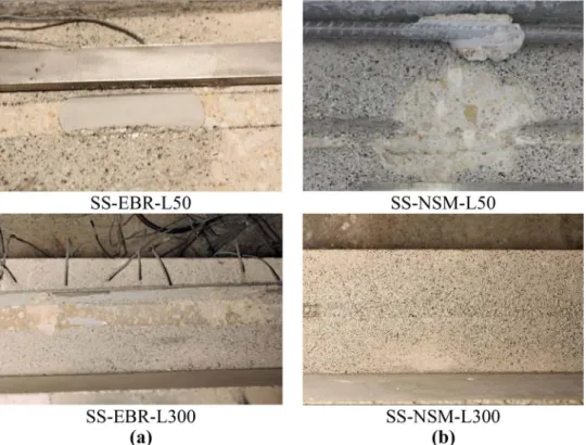
The common failure modes observed from the single-lap shear tests are briefly shown in Fig.6. In total, five different failure modes were observed and were classified as follows: (i) adhesive rupture of the stainless steel-to-resin interface (Type I); (ii) cohesive rupture within a surface layer of the concrete (Type II); (iii) mixed rupture, i.e. cohesive in con-crete and adhesive within the SS-to-adhesive interface (Type III); (iv) cohesive rupture within the concrete (Type IV); and (v) rupture of the stainless steel rod (Type V).
Mostly, the rupture observed in the EBR samples with shorter bond lengths was interfacial between the SS strip and the epoxy resin. However, as the bond length in these
specimens increased, the ruptures began to occur within a thin layer of concrete. In the NSM specimens tested, the failure modes observed with shorter or longer bond lengths were quite different. The failure mode detected in the sam-ples with shorter bond lengths were all cohesive within the concrete, whereas the rupture of the SS rod was observed in the two specimens with the longest bond length, i.e. with 200 and 300 mm. Comparing the EBR and the NSM tech-niques, the rupture of the SS observed in the NSM technique shows that this is more efficient than the EBR technique.
Despite being beyond the scope of this study, the failure modes herein observed show that an improvement to the EBR technique must be considered in the future. Amongst other possible solutions for increasing the bond strength capacity between the stainless steel and concrete, the installation of mechanical fasteners or adopting other inno-vative techniques (Almeida et al.2016) should be consid-ered. Of course, the best solution for achieving this would be one that is able to maximise the full mechanical behaviour of the SS strip. In other words, the ideal solution is the one that leads to the rupture of the strip. This has been achieved in recent studies with a new bonding technique designated as Continuous Reinforcement Embedded at Ends (CREatE) which was developed by the authors with other reinforcing materials (Biscaia et al. 2016c, 2017) and it consists to embed both free ends of the reinforcing material into the structural element.
Table3 presents the rupture modes observed and the rupture loads reached in each tested specimen. In Table3it can be seen that the rupture loads associated to the EBR technique tend to increase with the bond length and in the cases where this doesn’t occur the ruptures modes are mixed modes, i.e. parts of the bond length had adhesive failure within the SS-to-resin interface and other parts of the bond length ruptured within a superficial layer of concrete. Therefore, cohesive ruptures within the concrete are most efficient because, as should be expected from a bonding technique, the adhesive interfaces cannot be the weakest link in the bonding between two materials and the rupture should take place in one of the two bonded materials instead. For this reason, the NSM technique was considered the one that led to the best interface performance because the rupture of the SS rod was reached when a sufficient bond length was considered, i.e. 200 and 300 mm, with 48.9 kN (973 MPa) and 47.8 kN (951 MPa), respectively.
4. Accuracy of the DIC Technique
4.1 DIC vs. Strain Gauge-Based Measurements
The strains developed in the stainless steel strips bonded to the concrete accordingly to the EBR technique were all collected from the strain gauges bonded along the bond length. Since the strains developed in the stainless steel are much larger than those developed in the concrete, the strains developed in the concrete can be ignored. Therefore, the slips were determined based on the data collected from the
strain gauges according to (Biscaia et al. 2013; Ferracuti et al.2007):
s xð Þ ¼s xð iþ1Þ
eiþ1 ei
ð Þ
xiþ1 xi
ð Þ
xiþ1 x
ð Þ2
2 þeiþ1
ðxiþ1 xÞ ð2Þ
wherexcorresponds to the axis parallel to the bond length; (ei?1-ei) and (xi?1-xi) are, respectively, the strain and
the distance between two consecutive strain gauges.
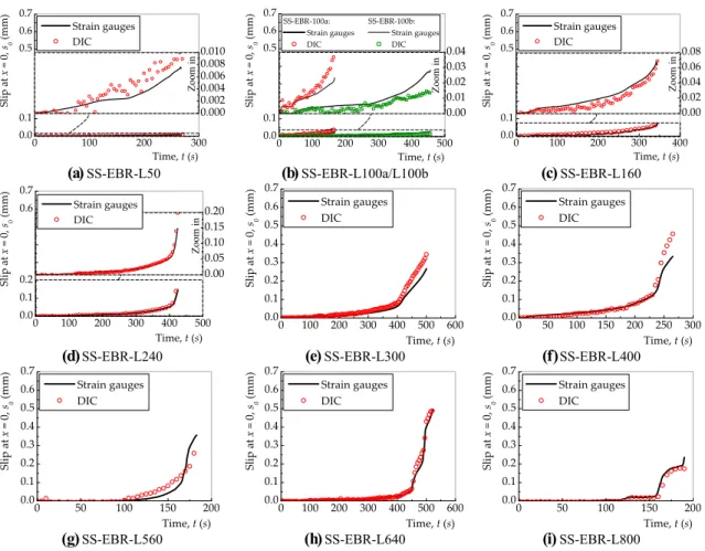
Thus, the slips obtained at the SS loaded end are either from Eq. (2) or from the DIC technique during the tests, i.e. the slip atx=Lbversus duration of the test is presented in Fig.7. As can be seen from this figure, the accuracy of the DIC technique with the slip derived from the strain gauges is
quite remarkable, especially in those specimens with larger bond lengths. However, a non-smooth slip distribution can be easily seen from the specimens with shorter bond lengths, i.e. with a bonded length shorter than the effective bond
Fig. 6 Common failure modes observed from the single-lap shear tests:aEBR samples; andbNSM samples.
Table 3 Rupture loads and rupture modes observed in the specimens.
Specimen Bond length,Lb(mm) Rupture loads,Frup(kN) Failure mode
SS-EBR-L50 50 6.3 Type I
SS-EBR-L100a 100 12.8 Type II
SS-EBR-L100b 100 12.4 Type I
SS-EBR-L160 160 14.5 Type I
SS-EBR-L240 240 15.9 Type II
SS-EBR-L300 300 21.9 Type II
SS-EBR-L400 400 18.6 Type III
SS-EBR-L560 560 14.6 Type III
SS-EBR-L640 640 18.5 Type II
SS-EBR-L800 800 14.8 Type III
SS-NSM-L35 35 13.8 Type IV
SS-NSM-L50 50 26.2 Type IV
SS-NSM-L75 75 35.6 Type IV
SS-NSM-L100 100 40.1 Type V
SS-NSM-L200 200 48.9 Type V
SS-NSM-L300 300 47.8 Type V
length, which induces a relevant noisy signal in determining the strains in the stainless steel.
In terms of relative displacements between materials, the Absolute Deviation (AD) and the Mean Absolute Deviation (MAD) between the DIC technique and the slips obtained from the strain gauge measurements were calculated in each test according to:
AD¼X
n
i¼1
sDIC0;i s0;i
ð3aÞ
and
MAD¼1
n
Xn
i¼1
sDIC0;i s0;i
ð3bÞ
wheres0and s0DICare the slips measured atx=0 obtained from Eq. (2) and from the DIC technique, respectively; and
nis the number of measurements carried out during the test. The results showed that the specimens with the shortest bond lengths have the lowest MAD, whereas the specimens with the longest bond lengths have the highest MAD. Thus, the lowest MAD was found in specimen SS-EBR-L50 with a calculated MAD of 0.002 mm and specimen SS-EBR-L560 had the highest MAD of 0.019 mm.
In terms of relative errors, the Absolute Percent Error (APE) and the Mean Absolute Percent Error (MAPE) were also determined according to:
APE¼100X
n
i¼1 sDIC
0;i s0;i
s0;i
ð4aÞ
and
MAPE¼100
n
Xn
i¼1
sDIC0;i s0;i
s0;i
: ð4bÞ
The results showed that the MAPE tends to decrease with the increase of the bond length adopted for the specimens. However, it is important to keep in mind that these results are very scattered but still, some tests showed that when the displacements increased the values for the MAPE tended to decrease. This may indicate that the use of the DIC tech-nique could be used if the displacements to be measured are not too small. Therefore, the use of the DIC technique may require some prudence and/or methodologies that should be considered for the experimental assessing of the bond between SS and concrete. In the following sections those aspects are highlighted and developed with the help of the samples initially considered in this work.
4.2 Load–Slip Response
The load–slip response of the stainless steel bonded to concrete will have different characteristics, depending if the bond length is longer or shorter than the effective bond 0 100 200 300
0.0 0.1 0.2 0.3 0.4 0.5 0.6 0.7
Time,t(s) Strain gauges DIC Sl ip at x =0 , s0 (m m) 0.000 0.002 0.004 0.006 0.008 0.010 Zo o m i n 0.00 0.01 0.02 0.03 0.04
0 100 200 300 400 500 0.0 0.1 0.2 0.3 0.4 0.5 0.6 0.7
Time,t(s)
Slip at x =0 , s0 (mm) SS-EBR-100a: SS-EBR-100b:
Strain gauges Strain gauges
DIC DIC Zoom in 0.00 0.02 0.04 0.06 0.08
0 100 200 300 400 0.0 0.1 0.2 0.3 0.4 0.5 0.6 0.7
Time,t(s) Strain gauges DIC Sl ip at x = 0, s0 (m m) Zoom in
(a)SS-EBR-L50 (b)SS-EBR-L100a/L100b (c)SS-EBR-L160
0.00 0.05 0.10 0.15 0.20
0 100 200 300 400 500 0.0 0.1 0.2 0.3 0.4 0.5 0.6 0.7
Time,t(s)
Sli p at x =0 , s0
(mm) Strain gaugesDIC
Zoom in
0 100 200 300 400 500 600 0.0 0.1 0.2 0.3 0.4 0.5 0.6 0.7
Time,t(s) Strain gauges DIC Sl ip at x =0 , s0 (mm)
0 50 100 150 200 250 300 0.0 0.1 0.2 0.3 0.4 0.5 0.6 0.7
Time,t(s) Strain gauges DIC Sl ip at x =0 , s0 (mm) 0 0 4 L -R B E -S S ) f ( 0 0 3 L -R B E -S S ) e (
0 50 100 150 200 0.0 0.1 0.2 0.3 0.4 0.5 0.6 0.7
Time,t(s) Strain gauges DIC Sl ip at x =0 , s0 (mm)
0 100 200 300 400 500 600 0.0 0.1 0.2 0.3 0.4 0.5 0.6 0.7
Time,t(s) Strain gauges DIC Sl ip at x = 0, s0 (mm)
0 50 100 150 200 0.0 0.1 0.2 0.3 0.4 0.5 0.6 0.7
Time,t(s) Strain gauges DIC Sl ip at x = 0, s0 (mm)
(d) SS-EBR-L240
(g) SS-EBR-L560 (h)SS-EBR-L640 (i)SS-EBR-L800
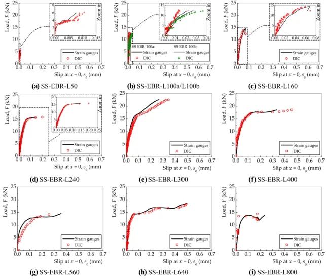
length. Thus, in order to help with the description of those differences, Fig.8 shows all the load–slip responses obtained from the EBR specimens. Moreover, the slips obtained from Eq. (1) and from the DIC technique are also shown in Fig.8. As already mentioned and previously demonstrated, the slips at the SS loaded end obtained either from the strain gauges or from the DIC technique are much alike. However, it seems that the slips measured from the DIC technique tend to deviate from the slips measured from the strain gauges in those EBR with SS specimens with the shortest bonded lengths. This was probably due to the very low values (\0.05 mm) of the slips involved in the
debonding processes of those EBR specimens (SS-EBR-L50, L100a, L100b and L160). If another digital camera with a better pixel resolution was used instead, then it would be sufficient to improve such measurements at such slip scale.
Nevertheless, both measurements are helpful for the defi-nition of the different states that the interface undergoes until its failure. For instance, in the EBR specimens with the longest bonded lengths, three different states can be identi-fied. In the order of their appearance in the load–slip curve they are easily characterized by: (i) an initial linear branch which corresponds to an elastic stage of the interface; (ii) a nonlinear branch which may correspond to a combined
elastic and softening stage of the interface; and (iii) a plateau that reveals the debonding initiation of the interface, i.e. the full detachment of the SS strip from the concrete. However, as the bond length decreases, these states tend to reduce and for too short bonded lengths it becomes probable to identify only the elastic stage from their load–slip responses.
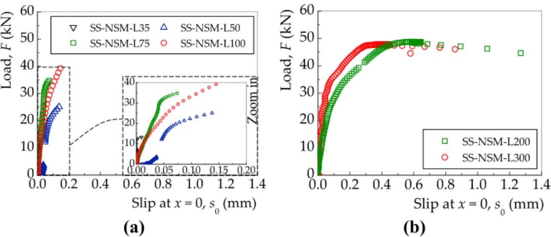
Much like the EBR specimens with SS strips, the load–slip response of the NSM specimens also allows three different states to be identified. Figure9 shows the load–slip responses obtained from the NSM samples. In Fig.9a, the load–slip responses of the shortest specimens are shown, whereas Fig.9b shows the responses of the specimens where the rupture of the SS rod occurred. Distinct from what happened in the EBR samples with the longest bonded lengths, where the plateau corresponds to the debonding propagation along the bond length, the plateau observed from specimens SS-NSM-L200 and SS-NSM-L300 corre-sponds to the yielding of the SS rod instead. So, the isolated and exclusive use of the DIC technique for the measure-ments of the displacemeasure-ments of the interface proved that by itself it is able to identify the distinct phases of the load–slip responses and the yielding stage of the NSM samples which helps provide better understanding in the analysis and interpretation of the interfacial behaviour between the SS and the concrete.
0.0 0.1 0.2 0.3 0.4 0.5 0.6 0.7 0 5 10 15 20 25 Lo ad, F (kN)
Slip atx= 0,s 0(mm) Strain gauges DIC
0.0000 0.005 0.010 0.015
2 4 6 8 Zo om in
0.0 0.1 0.2 0.3 0.4 0.5 0.6 0.7 0 5 10 15 20 25
Slip atx= 0,s 0(mm) Lo ad, F (kN) SS-EBR-100a: SS-EBR-100b:
Strain gauges Strain gauges
DIC DIC
0.00 0.01 0.02 0.03 0.040
5 10 15
Z
oom in
0.0 0.1 0.2 0.3 0.4 0.5 0.6 0.7 0 5 10 15 20 25 Lo ad, F (kN)
Slip atx= 0,s 0(mm) Strain gauges DIC
0.00 0.02 0.04 0.06 0.080
5 10 15
Z
oom in
0.0 0.1 0.2 0.3 0.4 0.5 0.6 0.7 0 5 10 15 20 25 Lo ad, F (kN)
Slip atx= 0,s 0(mm) Strain gauges DIC
0.00 0.05 0.10 0.15 0.20 0.250
5 10 15 20 Z oom in
0.0 0.1 0.2 0.3 0.4 0.5 0.6 0.7 0 5 10 15 20 25 Lo ad , F (kN)
Slip atx= 0,s 0(mm)
Strain gauges DIC
0.0 0.1 0.2 0.3 0.4 0.5 0.6 0.7 0 5 10 15 20 25 Lo ad , F (kN)
Slip atx= 0,s 0(mm)
Strain gauges DIC
0.0 0.1 0.2 0.3 0.4 0.5 0.6 0.7 0 5 10 15 20 25 Lo ad , F (kN)
Slip atx= 0,s 0(mm)
Strain gauges DIC
0.0 0.1 0.2 0.3 0.4 0.5 0.6 0.7 0 5 10 15 20 25 Lo ad , F (kN)
Slip atx= 0,s 0(mm)
Strain gauges DIC
0.0 0.1 0.2 0.3 0.4 0.5 0.6 0.7 0 5 10 15 20 25 Lo ad , F (kN)
Slip atx= 0,s 0(mm)
Strain gauges DIC
SS-EBR-L50 SS-EBR-L100a/L100b SS-EBR-L160
SS-EBR-L240 SS-EBR-L300 SS-EBR-L400
SS-EBR-L560 SS-EBR-L640
(a) (b) (c)
(d) (e) (f)
(g) (h) (i) SS-EBR-L800
4.3 Slips Developed Within the Interface
The relative displacements between bonded materials (or slips) developed along the bond length of the interface are analysed next, in accordance to Eq. (2). Whether for the sake of simplicity of the analysis or to avoid increasing the text unnecessarily, only two specimens were selected to be pre-sented, since the bond length of an interface has an important effect on its load–slip response: (i) the specimen with the largest bond length; and (ii) the specimen with the shortest bond length. Also, both strengthening bond techniques are contemplated in this analysis. Hence, Fig.10shows the slip distributions obtained from the specimens EBR-L50, SS-EBR-L800, SS-NSM-L35 and SS-NSM-L300. Furthermore,
the slips developed within the interface were calculated taking into consideration that:
s¼uss uc ð5Þ
whereussanducare the displacements in the stainless steel
and in the concrete. Thus, since the DIC Correlate software provides only the displacements, the slips measured using the DIC technique were calculated from the differences between the displacements measured along a line that embraces the bond length and another one that considers and measures the displacements along the concrete surface at the vicinity of the interface.
0.0 0.2 0.4 0.6 0.8 1.0 1.2 1.4 0
10 20 30 40 50 60
Loa
d,
F
(k
N) SS-NSM-L35 SS-NSM-L50 SS-NSM-L75 SS-NSM-L100
Slip atx= 0,s
0(mm)
0.00 0.05 0.10 0.15 0.200 10
20 30 40
Zoom
in
0.0 0.2 0.4 0.6 0.8 1.0 1.2 1.4 0
10 20 30 40 50 60
Lo
ad,
F
(kN
)
Slip atx= 0,s
0(mm)
SS-NSM-L200 SS-NSM-L300
(a)
(b)
Fig. 9 Load–slip responses of the NSM samples with:aa short bond length; andba long bond length.
0 5 10 15 20 25 30 35 40 45 50 0.000
0.005 0.010 0.015 0.020
Distance from the SS loaded end,x(mm) DIC
From strain gauges
S
lip,
s
(mm)
0 5 10 15 20 25 30 35 0.00
0.05 0.10 0.15 0.20
Distance from the SS loaded end,x(mm) DIC
Sli
p
,
s
(mm)
Short bond length, SS-EBR-L50 Short bond length, SS-NSM-L35
0 100 200 300 400 500 600 700 800 0.00
0.05 0.10 0.15 0.20 0.25
Distance from the SS loaded end,x(mm) 1
1 3
DIC
From strain gauges
Slip,
s
(mm)
2
1 2 3
0 50 100 150 200 250 300 0.0
0.1 0.2 0.3 0.4 0.5
Distance from the SS loaded end,x(mm) 3
2
DIC:
Slip
,
s
(mm)
1
1 2 3
Key: 1 - same slip value s0 observed in specimen
SS-EBR-L50 at failure; 2 - at approximately s0 = 0.1 mm; and 3 - at
the failure of the sample.
Key: 1 - same slip value s0 observed in specimen
SS-NSM-L300 at failure; 2 - at the initiation of the yielding of the rods; and 3 - at the failure of the sample.
Long bond length, SS-EBR-L800 Long bond length, SS-NSM-L300
) b ( )
a (
The slips developed within the EBR interface chosen to be presented in Fig.10a correspond to the debonding loads of the specimens and in the case of the EBR sample with the longest bonded length, an intermediate slip at x=0 was randomly selected. Therefore, the distribution corresponding to ‘‘1’’ in Fig.10a corresponds to the same slip at the SS loaded end when the debonding of the specimen SS-EBR-L50 occurred. In these cases, the results obtained either from the strain gauges or from the DIC technique are presented. Despite the noisy signal obtained from the DIC technique, the comparison between the two monitoring methods at least allows us to check the capability of the DIC to follow the same trend obtained from the strain gauges. Thereby, the results shown in Fig.10a indicate that the DIC technique is capable of following the same slip distributions of those obtained from Eq. (2), i.e. with highest slips at the SS loaded end with a decrease of the slips towards the SS free end.
The same criterion was followed in Fig.10b to show the slip distributions obtained from the NSM selected samples. However, the middle slip distribution in the specimen SS-NSM-L300 corresponds to the initiation of the yielding of the SS rod (see Fig.10b). As can be seen from these results, a relevant discontinuity of the slip distribution can be observed at the vicinities of the SS loaded end, which is explained by the yielding of the SS rod. At the same time, the slip distributions corresponding to numbers ‘‘2’’ and ‘‘3’’ are quite similar, which can be explained, once again, by the yielding of the SS rod outside of the bonded length. Thus, when the SS rod yields, the load transmitted to the SS rod remains the same and the slips along the bond length should remain almost unchanged from then. Consequently, the displacements increase elsewhere outside the SS-to-concrete interface and the failure will also be localized there.
4.4 Axial Stresses and Strains Developed in the Stainless Steel
As mentioned above, the distribution of strains in the stainless steel used on the EBR samples was obtained from the strain gauges. In addition to the measurements collected from the strain gauges, the strains in the stainless steel were also measured with the DIC technique. However, as shown in the previous subsection, the slips obtained from the DIC technique are not quite smooth enough to obtain a smooth strain distribution. Consequently, the axial stress distribu-tions obtained from both measurements are not much alike, as shown in Fig.11a. Besides that, from Fig. 11it can also be seen that the maximum axial stress in the stainless steel used on the EBR with SS specimens and measured by the strain gauges is quite far away from its rupture value. Therefore, the mechanical properties of the stainless steel were not fully used, which shows how inefficient the EBR technique is. However, using the DIC technique, the maxi-mum axial stress was, as expected due to its long bonded length, registered in specimen SS-EBR-L800, which reached 271.0 MPa at 190 mm away from the SS loaded end.
In the NSM samples, the axial stress distributions are at least consistent with what would be considered acceptable, i.e. the axial stresses developed in specimens SS-NSM-L35
are almost uniform and didn’t reached the yielding value of the SS rod. The debonding failure process of short bonded lengths is characterized by a slip distribution where there are no undeformed bonded regions (see Fig.10). In addition, from the first derivative of Eq. (5) with respect to x and ignoring the strains developed in the concrete, it could be concluded that there are no regions where the strains could be zero unless, of course, precisely at the SS free end, where there are no assigned external loads to the stainless steel.
In sum, and despite the differences and the procedures that are needed to overcome the difficulties raised by the use of the DIC technique, the overall view of the results obtained with this monitoring technique is positive. In particular, the fact that several aspects observed in the experiments were identified and validated by the DIC technique. Even when the yielding of the SS rod was observed in specimen SS-NSM-L300, the DIC technique was capable of predicting this as shown in the graph at the bottom of Fig.11b.
5. Data Interpretation
In this section, the experimental results are discussed and analyzed. Based on the experiments, the effective bond length, i.e. the length beyond which the debonding load cannot increase any more, is defined as the debonding load vs. bond length graph. Moreover, the interfacial bond–slip relationships obtained from the experiments both from the EBR system or NSM system are herein presented.
5.1 Definition of the Effective Bond Length
The notion of effective bond length (Leff) of an interface is
rods. Thus, in the case of the EBR system, the effective bond length was found to be 235 mm, whereas the NSM system showed an effective bond length of 168 mm. Based on these results and regarding the maximum loads reached in both cases, the NSM system with stainless rods showed itself to be the best bonding system in this case too because a clas-sical rupture in the stainless steel is reached for a lower effective bond length than that estimated by the EBR system with SS strips.
Despite being beyond the purpose of this work, the per-formance of the EBR systems can be improved by using an additional anchorage system. This issue is of great impor-tance, as can be attested to by the numerous researches found in the literature (Biscaia et al.2014; Mendes2008; Martinelli
et al.2012; Bren˜a and McGuirk2013; Realfonzo et al.2013; Wu and Liu2013) seeking for a valid and alternative solu-tion for enhancing the strength of EBR systems. Still, it is important to bear in mind that the use of steel mechanical fasteners involves making a hole on the SS strip which may lead to an important setback due to the reduction of the SS cross section of the strip to install the fasteners. Conse-quently, the rupture load of the stainless strip is reduced. Therefore, an alternative method to anchor the stainless steel is recommended instead and in this way, the innovative CREatE technique developed by the authors (Chastre et al. 2016; Biscaia et al. 2016c, 2017) using CFRP laminates instead of SS strips could be an important contribution to this topic because once the FRP or the SS free ends are embedded in concrete, the rupture of the FRP composite or the yielding of the SS are always reached.
5.2 Interfacial Bond–Slip Relationship
of the EBR System
To determine the local bond–slip relationship between the stainless steel and concrete, the bond stress developed within the interface is obtained from the equilibrium of an infinitesimal lengthdxof the SS-to-concrete interface, which gives the following equation:
sð Þ ¼x tss
drss
dx ð6Þ
wheretssis the thickness of the stainless steel anddrss/dxis
the variation of the axial stress in the stainless steel in the infinitesimal lengthdx. The determination of the bond stress
0 10 20 30 40 50
0 100 200 300 400 500 600 700 Rupture stress DIC Strain gauges
Bond length,L
b(mm) Axi al st ress in the SS , SS (MP a) Yielding stress
0 5 10 15 20 25 30 35 0 150 300 450 600 750 900 1050 DIC
Bond length,L
b(mm) Axial stress in the SS, SS
(MPa) Yielding stress
0 100 200 300 400 500 600 700 800 0 100 200 300 400 500 600 700 Rupture stress DIC Strain gauges
Bond length,L
b(mm) Axial stre ss in th e SS , SS (M Pa ) Yielding stress
0 50 100 150 200 250 300 0 150 300 450 600 750 900 1050 DIC
Bond length,L
b(mm) Axial stre ss in th e S S, SS (M Pa ) Yielding stress
Short bond length, SS-EBR-L50 Short bond length, SS-NSM-L35
Long bond length, SS-EBR-L800 Long bond length, SS-NSM-L300
) b ( ) a ( σ σ σ σ
Fig. 11 Stresses developed in the stainless steel obtained from:aEBR samples; andbNSM samples.
0 100 200 300 400 500 600 700 800
0 10 20 30 40 50 60 EBR technique NSM technique
Bond length,L b(mm) Maximum loa d , F max
(kN) Rupture of the SS rebar
between two consecutive strain gauges was accomplished through the axial stressed developed in the stainless steel in which Eq. (1) was used. So, Eq. (6) can be rewritten as a function of the difference between two consecutive calculated axial stresses:
s xiþ1=2
¼tss
rss;iþ1 rss;i
xiþ1 xi
ð7Þ
where (rss,i?1-rss,i) and (xi?1-xi) are, respectively, the
stress in the stainless steel and the distance between two consecutive points. It is worth keeping in mind that Eq. (7) assumes, therefore, that the bond stresses developed between two consecutive points are constant and, in order to ensure a precise calculation of the bond stress, it is important to avoid high distances (xi?1-xi) and distances shorter than 50 mm
are recommended.
The slip distribution is determined by Eq. (2) and the bond–slip relationship is then determined by coupling the bond stress calculated from Eq. (6) and the average slip obtained from:
s xiþ1=2
¼s xð iþ1Þ þs xð Þi
2 ð8Þ
wheres(xi?1) is the slip at pointxi?1ands(xi) is the slip at
pointxi.
Figure13 shows the interfacial bond–slip relationships obtained from EBR with SS specimens with a bond length greater than the effective bond length, i.e. over 235 mm. In each specimen, the different curves are presented and each one corresponds to the mid-point of an interval between two consecutive strain gauges at a fixed distance from the SS loaded end. Despite some visible differences between sam-ples, the results show that the bond–slip relationships have some points in common. For instance, for every single specimen, an initial increase of the bond stress is observed until a maximum bond stress is reached. This first stage is usually designated in the literature (e.g. Martinelli et al. 2011; Dehghani et al. 2012; Biscaia et al.2013,2014; Xia and Teng2005) as an elastic stage. After this elastic stage, a softening and nonlinear stage develops. The shape of this softening stage is not always the same and, for instance in specimens SS-EBR-L240, SS-EBR-400 and SS-EBR-L800 the softening stage seems to be quite symmetric with the elastic stage, whereas in the other samples the softening stage decays quickly after the maximum bond stress value and tends to be almost parallel to thex-axis as the slip within the interface approaches its ultimate value. The debonding stage, i.e. the stage with zero bond stress transfer, is not clearly observed in any of the EBR specimens studied here. Also the maximum bond stress and its corresponding max-imum slip developed within the interface was not always the same.
5.3 Interfacial Bond–Slip Relationship of the NSM System
Unlike the EBR specimens with stainless steel which were monitored with several strain gauges, the NSM specimens were monitored only with the DIC technique. Hence, the relative displacement within the SS-to-concrete interface measured with the DIC technique was the only information gathered from the single-lap shear tests carried out in this work. For this reason, the methodology followed in the previous section for determining the interfacial bond–slip relationship of the EBR samples cannot be used in this case of NSM specimens. The methodology followed in this sit-uation is described next and it was based on the strain vs. slip curve obtained from the test at the SS loaded end (@
x=0). This methodology was proposed by Dai et al. (Dai et al.2005) and has been used since then by the authors with good results (Biscaia et al. 2016c, 2017) to evaluate the bond–slip relationship developed within an FRP-to-concrete interface. To determine the interfacial bond–slip relationship, this method requires that the slip and bond stress measure-ments at one specific point, which, in the present case, corresponds tox=0. Hence, for the current NSM samples, the prediction of the interfacial bond–slip relationship of the SS-to-concrete interface begins by considering, once more, the equilibrium of a segment dx, leading to the following equation (Biscaia et al.2015a,b):
sð Þ ¼x /ss
4
drss
dx ð9Þ
where/ss is the diameter of the stainless steel rod. Eq (9)
can be rewritten as:
sð Þ ¼x /ss 4
drss
ds
ds
dx ð10Þ
where ds/dx is defined as the strain in the stainless steel, since the strains developed within the concrete are ignored due to their negligible values when compared to the strains developed in the stainless steel. Therefore, Eq. (10) can be rewritten as a function of the axial stresses and strains in the SS according to:
sð Þ ¼s /ss
4
drss
ds ess ð11Þ
whereessis the strain in the stainless steel. Eq (11) is then
numerically solved according to:
sið Þ ¼s /ss
4
rss;iþ1 rss;i 1 s0;iþ1 s0;i 1
ess;i ð12Þ
already defined in Sect.2, the interfacial bond–slip rela-tionship is obtained. As already shown from the EBR sam-ples, the DIC technique is capable of reasonably reproducing the slips within the interface at the most loaded regions. Taking into account the stresses in the SS rod obtained from the load pressure cell, the reproduction of the stress versus slip curve at the SS loaded end is defined and, based on the stress versus strain behaviour of the SS, the interfacial bond– slip relationship is predicted by Eq. (12). Still, when it comes to the differentiating a noisy signal such as that obtained from the strain distribution in the stainless steel (see Sects. 4.3 and 4.4), the results will have an even nosier signal and that is why an exponential smoothing with a smooth constant ofa=0.2 was used in this case, in order to smooth out the ‘‘peaks and valleys’’ found in the results obtained from Eq. (12) and to show their trend is close to the real curve. Hence, Fig.14 shows the smoothed results for the interfacial bond–slip relationships obtained from all the
NSM specimens. Based on these results, it can be seen that despite the visible differences, the bond–slip relationship determined in the NSM samples has an initial elastic stage,
(a)
(c)
(d)
(e)
(f)
(b)
Fig. 13 Interfacial bond–slip relationships of the EBR samples obtained from the strain gauges.
as well. However, at the end of this elastic stage, the bond– slip relationships in the NSM samples seems to show a plateau at a peak bond stress value and then, the bond stress decays until it reaches a zero value. Thereof, bond–slip relationships such as elastic with fragile rupture, rigid-plas-tic, rigid with linear softening or other reported in (Biscaia et al.2013) are herein excluded and a trapezoidal shape may describe better, even if approximately, the interfacial beha-viour shown in the NSM samples. In terms of the values of the nuclear points needed to define the bond–slip relation-ship, it can be stated that the maximum bond stress deter-mined from the NSM samples approximately reached 20.0 MPa. Moreover, the maximum slip, i.e. the slip at maximum bond stress, determined in the NSM samples is approximately 0.2 mm more than the maximum slip calcu-lated in the EBR samples.
5.4 Interfacial Bond–Slip Relationships: EBR System Versus NSM System
Based on the two NSM samples that failed due to the rupture of the SS rod (specimens NSM-L200 and SS-NSM-L300), it seems that the full detachment of the SS rod from the concrete occurs at a finite ultimate slip (sult),
whereas in the EBR samples the separation between mate-rials takes place with a smoother transition. To help in these comparisons, Fig.15 shows both curves where the bond– slip relationship determined either from the NSM samples or from the EBR samples are represented by areas limited by their minimum and maximum values. As can be seen from Fig.15, the differences between both interfacial behaviours are different.
Given the differences found here, the use of the NSM bonding technique by itself is not sufficient to justify those differences. Still, conjugated with the NSM bonding tech-nique, the use of ribbed stainless steel rods may justify such differences in the bond stress transfer between samples with different bonding techniques because the ribs increase the friction within the interface leading to the improvement of the bond stress transfer between materials. In fact, in Model Code 2010 (Fe´de´ration Internationale du Be´ton 2010), the influence of the steel rib area is recognized as one of the aspects that significantly affects the bond–slip relationship. Moreover, a trapezoidal shape of the bond–slip relationship
to simulate the local bond behaviour between a ribbed steel rod and concrete is a possibility that is covered in Model Code 2010 (Fe´de´ration Internationale du Be´ton2010).
The mid-curves shown in Fig.15are intended to represent the interfacial bond–slip relationships of each bonding technique studied here. Based on the maximum and mini-mum values obtained from each bonding technique, the mid-range curves in Fig.15 are intended to cover a mid-range value for the EBR and the NSM bonding techniques. Hence, the mid-range bond–slip relationship for the EBR bonding technique is defined according to (Popovics1973):
sð Þ ¼s smaxn
n 1
ð Þ þ s smax
n
s smax
ð13Þ
wheresmaxis the maximum bond stress; smax is the slip at maximum bond stress; andn is a constant to be defined in order to approximate the shape of the bond–slip relationship to the experimental results. The mid-range values needed for the definition of Eq. (13) are: smax=9.0 MPa,
smax=0.031 mm and n =2.5. The mid-range bond–slip curve for the NSM bonding techniques is defined according to:
sð Þ ¼s
smax
smax;1 if 0ssmax;1 smax if smax;1\ssmax;2
smax
smax;2 smax;1ðsult s2Þ if smax;2
\ssult
0 if s[sult
8 > > <
> > :
ð14Þ
wheresmax,1andsmax,2are, respectively, the slips at the end of the elastic stage and at the end of the constant stage; and
sultis the ultimate slip, i.e. the slip beyond which no further
bond transfer between materials is ensured. For the defini-tion of Eq. (14) shown in Fig.15, a mid-range value for the maximum bond stress was foundsmax=16.3 MPa and with slips smax,1=0.060 mm, smax,2=0.280 mm and sult=
0.500 mm.
6. Conclusions
An experimental work was developed in order to study the performance of stainless steel strips and rods bonded to concrete. As well as the use of strain gauges to determine the interfacial bond–slip relationship between the stainless steel and the concrete, the DIC technique was also used which allowed a bonded area to be analysed instead of a local strain provided by the use of single strain gauges. As an overview of the results achieved, the following conclusions can be made:
• The use of ribbed SS rods showed that it is possible to
obtain the rupture of the rod if an appropriate bonded length is used. In the present experimental work, it was found that for 200 mm the rupture of the SS rod is reached. Thereby, the premature debonding phenomenon
of the SS rod is avoided and the mechanical properties of the SS rod are fully used;
• the EBR samples performed poorly when compared to
the NSM samples. In all the tests carried out, the premature debonding of the SS strip was observed at a strain somewhat lower than its rupture value. In the EBR samples with a short bond length, i.e. with a bonded length shorter than the effective bond length, the rupture occurred within the SS-to-adhesive interface, which means that the resin has poor properties for bonding SS strips. However, when the bond length of the SS-to-concrete interface increases, a mixed failure mode was observed with the separation of a thin layer of concrete from the substrate with 2–3 mm of depth and, at the same time, with an adhesive rupture within the SS-to-adhesive interface;
• the DIC technique can be used, although carefully, to
evaluate the bond transfer between the SS and concrete. The displacements measured with the DIC technique and the slips calculated from these results were reasonably well estimated. Mainly when those values were greater than one tenth of a millimetre, the DIC proved to be capable of predicting the results fairly well. However, the noisy signal obtained for the slips make it difficult to determine the strains and bond stresses due to its higher order, i.e. due to the first and second derivatives of the slips with respect tox(axis parallel to the bond length) for the calculation, respectively. Still, the methodologies followed permitted the yielding of the SS rods in the NSM samples to be identified and allowed us to get a fair perspective of the strain distribution in the SS strip in the EBR samples;
• the DIC technique also allowed the load–slip distribution
to be captured accurately. This weighs heavily in the evaluation of the bond between two materials because, based on the load–slip response, the interfacial behaviour can be predicted. Thus, depending on the load–slip response until failure, the different stages that character-ize the bond–slip relationship can be estimated. For instance, an initial linear load–slip response means that the interfacial bond–slip relationship has a linear and elastic stage as well. Afterwards, the nonlinear load–slip response observed from the samples means that the interfacial bond–slip relationship has a softening stage. This transition between the linear and the nonlinear load–slip response corresponds to a maximum bond stress value of the bond–slip relationship;
• The effective bond length of the EBR samples was
235 mm, whereas the NSM samples had an effective bond length of 168 mm, which represents 71.5% of the value obtained for the EBR samples;
• the bond–slip relationships obtained for the two types of
samples studied here are different. In the EBR samples, a power function was able to describe a mid positioning of the experimental bond stresses (i.e. the corresponding mid-range values between the maximum and the mini-mum experimental bond stresses) obtained along the slips within the interface at the SS loaded end. However,
in the NSM samples, a trapezoidal shape to describe the bond–slip relationship was proposed to approximate the experimental findings. Comparing the limit points of both bond–slip relationships, it can be concluded that the mid-range maximum bond stress found for the NSM samples reached 1.8 times of that found for the EBR samples. In term of slips, the NSM samples had higher values with the mid-range value of the ultimate slip developed within the interface of the NSM samples being approximately 0.5 mm, whilst an ultimate slip of 0.4 mm was never exceeded in the EBR samples.
Acknowledgements
The first author of this work would like to express his deepest gratitude to Fundac¸a˜o para a Cieˆncia e Tecnologia for the partial financing of this work under the UNIDEMI Strategic Project PEst-OE/EME/UI0667/2014 and for the post-doctoral grant SFRH/BPD/111787/2015. The second author is also grateful to UNIDEMI for his scientific research grant under the Strategic Project UID/EMS/ 00667/2013.
Open Access
This article is distributed under the terms of the Creative Commons Attribution 4.0 International License (http:// creativecommons.org/licenses/by/4.0/), which permits unre stricted use, distribution, and reproduction in any medium, provided you give appropriate credit to the original author(s) and the source, provide a link to the Creative Commons license, and indicate if changes were made.
References
AG, & SPCRC. (2016).S&P Resin 220(p. 2).
Aiello, M., & Leone, M. (2008). Interface analysis between FRP EBR system and concrete.Journal of Composites Part B: Engineering, 39(4), 618–626.
Akbar, I., Oehlers, D. J., & Ali, M. S. M. (2010). Derivation of the bond–slip characteristics for FRP plated steel members.
Journal of Constructional Steel Research, 66(1–8), 1047–1056.
Almeida, G., Melı´cio, F., Biscaia, H., Chastre, C., & Fonseca, J. M. (2016). In-plane displacement and strain image analysis.
Computer-Aided Civil and Infrastructure Engineering, 31(4), 292–304.
Al-Mosawe, A., Al-Mahaidi, R., & Zhao, X.-L. (2015). Effect of CFRP properties, on the bond characteristics between steel and CFRP laminate under quasi-static loading. Con-struction and Building Materials, 98,489–501.
Aykac, S., Kalkan, I., Aykac, B., Karahan, S., & Kayar, S. (2013). Strengthening and repair of reinforced concrete beams using external steel plates. Journal of Structural Engineering, 139(6), 929–939.
Biscaia, H. C., Chastre, C., Borba, I. S., Silva, C., & Cruz, D. (2016a). Experimental evaluation of bonding between CFRP laminates and different structural materials.Journal of Composites for Construction, 20(3), 04015070. Biscaia, H., Chastre, C., Cruz, D., & Franco, N. (2017a).
Flexural strengthening of old timber floors with laminated carbon fiber reinforced polymers. Journal of Composites for Construction, 21(1), 04016073.
Biscaia, H. C., Chastre, C., Cruz, D., & Viegas, A. (2017b). Prediction of the interfacial performance of CFRP lami-nates and old timber bonded joints with different strengthening techniques.Composites Part B Engineering, 108,1–17.
Biscaia, H. C., Chastre, C., & Silva, M. A. G. (2013a). Non-linear numerical analysis of the debonding failure process of FRP-to-concrete interfaces. Composites Part B Engi-neering, 50,210–223.
Biscaia, H. C., Chastre, C., & Silva, M. A. G. (2013b). Linear and nonlinear analysis of bond–slip models for interfaces between FRP composites and concrete.Composites Part B Engineering, 45(1), 1554–1568.
Biscaia, H. C., Chastre, C., Silva, C., & Franco, N. (2017c). Mechanical response of anchored FRP bonded joints: A nonlinear analytical approach. Mechanics of Advanced Materials and Structures. https://doi.org/10.1080/ 15376494.2016.1255812.
Biscaia, H. C., Chastre, C., Viegas, A., & Franco, N. (2015a). Numerical modelling of the effects of elevated service temperatures on the debonding process of frp-to-concrete bonded joints.Composites Part B: Engineering,70, 64–79. Biscaia, H. C., Chastre, C., & Viegas, A. (2015b). A new dis-crete method to model unidirectional FRP-to-parent mate-rial bonded joints subjected to mechanical loads.
Composite Structures, 121,280–295.
Biscaia, H. C., Cruz, D., & Chastre, C. (2016b). Analysis of the debonding process of CFRP-to-timber interfaces. Con-struction and Building Materials, 113,96–112.
Biscaia, H. C., Franco, N., Nunes, R., & Chastre, C. (2016c). Old suspended timber floors flexurally-strengthened with different structural materials. Key Engineering Materials, 713,78–81.
Biscaia, H. C., Micaelo, R., Teixeira, J., & Chastre, C. (2014). Numerical analysis of FRP anchorage zones with variable width.Composites Part B Engineering, 67,410–426. Bizindavyi, L., & Neale, K. W. (1999). Transfer lengths and
bond strengths for composites bonded to concrete. ASCE Journal of Composites for Construction, 3(4), 153–160. Blaschko, M., & Zilch, K. (1999). Rehabilitation of concrete
structures with CFRP strips glued into slits. In: ICCM-12, I.—I.C.O.C. Materials. Paris, France: ICCM.
Bren˜a, S. F., & McGuirk, G. N. (2013). Advances on the behavior characterization of FRP-anchored carbon fiber-reinforced polymer (CFRP) sheets used to strengthen
concrete elements. International Journal of Concrete Structures and Materials, 7(1), 3–16.
Caggiano, A., Martinelli, E., & Faella, C. (2012). A fully-ana-lytical approach for modelling the response of FRP plates bonded to a brittle substrate.International Journal of Solids and Structures, 49(17), 2291–2300.
Carrara, P., Ferretti, D., Freddi, F., & Rosati, G. (2011). Shear tests of carbon fiber plates bonded to concrete with control of snap-back. Engineering Fracture Mechanics, 78,
2663–2678.
CEN, EN ISO 6892-1:2009. (2009). Metallic materials. Tensile testing—Part 1: Method of test at ambient temperature,
CEN.
CEN, NP EN 12390-3. (2003).Ensaios de beta˜o endurecido: Resisteˆncia a` compressa˜o dos provetes de ensaio. Instituto Portugueˆs da Qualidade (in Portuguese).
Chastre, C., Biscaia, H., & Franco, N. (2017). Strengthening of RC beams with post-installed steel bars or FRP composites.
Mecaˆnica Experimental, 28,39–46. (in Portuguese). Chastre Rodrigues, C. Behaviour of steel-epoxy-soncrete
con-nection in structural elements.MSc thesis, Instituto Supe-rior Te´cnico; 209 pp. (in Portuguese).
Chastre, C., Biscaia, H. C., Franco, N., & Monteiro, A. (2016). Experimental analysis of reinforced concrete beams strengthened with innovative techniques. In: 41st IAHS WORLD CONGRESS Sustainability and Innovation for the Future (pp. 1–10), 13–16 September 2016, Albufeira, Portugal.
Chen, J. F., Yuan, H., & Teng, J. G. (2005). Analysis of debonding failure along a softening FRP-to-concrete interface between two adjacent cracks. In: Chen, J. F., & Teng, J. G. (Eds.), Proceedings of the International Sym-posium on Bond Behaviour of FRP in Structures, BBFS 2005(pp. 103–111).
Cruz, J. R., Borojevic, A., Sena-Cruz, J., Pereira, E., Fernandes, P. M. G., Silva, P. M. and Kwiecien, A. (2016). Bond behaviour of NSM CFRP-concrete systems: adhesive and CFRP cross-section influences. In: Eighth International Conference on Fibre-Reinforced Polymer (FRP) Compos-ites in Civil Engineering (CICE2016).
Czaderski, C., Soudki, K., & Motavalli, M. (2010). Front and side view image correlation measurements on FRP to concrete pull-off bond tests. Journal of Composites for Construction, 14(4), 451–463.
Dai, J., Ueda, T., & Sato, Y. (2005). Development of the non-linear bond stress–slip model of fiber reinforced plastics sheet-concrete interfaces with a simple method.Journal of Composites for Construction, 9(1), 52–62.
De Lorenzis, L., Nanni, A., & Tegola, A. (2000). Strengthening of reinforced concrete structures with near surface mounted FRP rods. In: International Meeting on Composite Mate-rials, PLAST 2000, Milan, Italy.