Fiscal vulnerability in Brazil: a simulated method of moments approach

Ensaios Econômicos

EPGE

Escola

Brasileira de

Economia e

Finanças

N

₈₀₀

_{ISSN 0104-8910}

Fiscal Vulnerability in Brazil:

a Simulated

Method of Moments Approach

Eduardo Lima Campos, Rubens Penha Cysne

Agosto de 2018

URL:

http://hdl.handle.net/10438/24713

Os artigos publicados são de inteira responsabilidade de seus autores. As

opiniões neles emitidas não exprimem, necessariamente, o ponto de vista da

Fundação Getulio Vargas.

EPGE Escola Brasileira de Economia e Finanças

Diretor Geral: Rubens Penha Cysne

Vice-Diretor: Aloisio Araujo

Diretor de Regulação Institucional: Luis Henrique Bertolino Braido

Diretores de Graduação: Luis Henrique Bertolino Braido & André Arruda Villela

Coordenadores de Pós-graduação Acadêmica: Humberto Moreira & Lucas Jóver Maestri

Coordenadores do Mestrado Profissional em Economia e Finanças: Ricardo de Oliveira

Cavalcanti & Joísa Campanher Dutra

Lima Campos, Eduardo

Fiscal Vulnerability in Brazil:

a Simulated Method of

Moments Approach/ Eduardo Lima Campos, Rubens Penha Cysne – Rio

de Janeiro :

FGV,EPGE, 2018

36p. - (Ensaios Econômicos; 800)

Inclui bibliografia.

Fiscal Vulnerability in Brazil: a Simulated

Method of Moments Approach

Eduardo Lima Campos1 Rubens Penha Cysne2

Abstract This article estimates a structural macroeconomic model of the Brazilian

economy, with emphasis on the exchange rate, interest rate, inflation and public debt risk premium. The aim is to assess the effect of different fiscal trajectories on the solvency of the public debt and possible episodes of fiscal vulnerability (defined here as a situation where the government’s fiscal precariousness prevents the central bank, in certain contexts, from reducing inflation by raising the basic interest rate). The change in relation to the usual case is the inclusion of a measure of the endogenous variation of the debt risk premium. To get around the usual problem of endogeneity in estimating a system of structural equations, we use the simulated method of moments (McFadden, 1989). Besides being more flexible than the techniques usually applied in the literature, this method enables stochastic projections under different macroeconomic settings to be obtained. We use alternative fiscal scenarios, associating each one with different likelihoods of fiscal vulnerability generated by the resulting distinct evolutions of the debt/GDP ratio.

Keywords Fiscal Vulnerability · Fiscal Dominance · Simulated Method of Moments · Interest Rates · Pass-Through · Exchange Rate · Inflation

JEL Classification H 30, H 60, E 50.

1 _{Professor at ENCE/IBGE and FGV/EPGE. E-mail: [email protected]} 2 _{Professor at FGV/EPGE. E-mail: [email protected]}

1

Introduction

Countries that combine inflation targeting with flexible exchange rates in an environment of fiscal laxity and high public debt/GPD ratios, with a short average maturity, are always subject to a possible problem: raising the basic interest rate beyond a certain point can signal an increased probability of either partial or total debt default.

Default scenarios are generally based on the political and institutional difficulties of cutting spending and/or increasing revenues during a period of financial difficulty for the public sector. This casts doubt on the government’s capacity to service its debt. When the possibility of default is explicitly considered by savers, an interest rate hike may not be sufficient to make this debt more attractive, and in extreme cases it can reduce demand for sovereign bonds.

The possibility of default reduces the attractiveness of the debt in relation to a risk-free investment in at least three ways. First, it diminishes the expected future receipt not only of interest, but also the principal. Second, it introduces uncertainty regarding the yield of the bond. Depending on the saver’s risk aversion, this second aspect can have a significant impact on the attractiveness of the debt. Third, the prospect of default is also the prospect of a crisis, with lower GDP growth and consequently smaller tax revenue flows in the future. This reasoning is stronger the more rigid public spending is.

All these factors obviously tend to deteriorate the evolution of the debt even more, an important aspect for the initial conjecture about the chance of default. They tend to corroborate initial expectations.

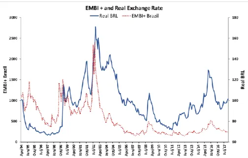
Theoretically, when the exchange rate regime is flexible and a reasonable part of the net debt is denominated in foreign currency (not the case of Brazil right now and in the recent past), an additional perverse effect can occur. If the risk aversion of foreign savers is higher than the market average, the incorporation of the prospect of default by the market equilibrium rate may not be sufficient to maintain the external attractiveness of the country’s sovereign debt. The flow of capital to the country will then decline, causing the real exchange rate to depreciate and increasing the debt service cost. Once again the debt dynamic deteriorates, supporting the initial expectation of default.

Figure 1.1 shows the evolution of the real exchange rate and risk premium in Brazil (measured here by the EMBI+ Brazil) between 1994 and 2017, suggesting dependence on the exchange rate:

Fig. 1.1 Real exchange rate and EMBI+ in Brazil between April 1994 and December 2017

Alternatively, when the exchange rate regime is flexible and the country adopts a rigid program of inflation targeting without support from fiscal policy, the same perverse dynamic can occur regardless of the amount of debt denominated in foreign currency. Once again, in the presence of foreign savers with greater risk aversion than the market average, the increased prospect of default (and consequent response of the central bank in raising the basic interest rate) can weaken the domestic currency instead of strengthening it.

This devaluation raises internal prices of importable and exportable goods. There is no certainty that this will increase inflation, since the initial elevation of the interest rate will also work to reduce prices through its negative impact on investments (along with sales of consumer goods and inventories) and aggregate demand, and hence on employment and wages.

It so happens that without the help of the exchange rate (via appreciation), the demand channel may not be sufficient to counteract the inflationary effects of the devaluation. If the central bank, in these adverse circumstances, insists on raising the interest rate again, it may create a perverse dynamic that deteriorates the expected path of the public debt, and thus reinforces the expectation of default.

For all these reasons it is very important to understand which variables should be monitored to guide actions to prevent the economy from facing the situation described,

in which an initial expectation of default is reinforced by changes in economic fundamentals that create a negative feedback effect.

The perverse dynamic between interest rate and exchange rate occurs, as described, when an increase in the basic interest rate by the central bank generates a weaker exchange rate (increase in the reference price of foreign currency) instead of appreciation.

In the literature, the expression “fiscal dominance” has been used to describe a mechanism similar to that depicted here. However, the concept of fiscal dominance used originally by Sargent and Wallace (1981), although very precise, is hard to characterize in practice. With a certain freedom of expression, here we alternatively define “fiscal vulnerability”, as a situation where, due to increased expectation of default, a rise in the interest rate winds up increasing instead of decreasing inflation.

This happens when the rise of prices implied by the perverse dynamic between the interest rate and exchange rate (with consequent weakening of the exchange rate with monetary tightening) outweighs the conventional effects of the interest rate on aggregate demand and prices. That dynamic does not necessarily have to be irreversible in time or linear with the elevation of the interest rate.

Against this backdrop, the economy is in a situation where only an improvement of the fiscal situation can be effective to control inflation, hence our use of “vulnerability”. When this fiscal vulnerability or dominance is established in moments of crisis, doubt is cast on the previous perception about fighting inflation through increasing the interest rate.

It has long been recognized that under conditions of fiscal leniency the use of monetary policy can be undermined. In this situation, a policy of raising the interest rate, by spurring growth of the debt, might only delay (and aggravate) the inflation problem over the long run. A momentaneous partial default can be associated with this rise of inflation due to the imperfect indexation of public bonds.

When looking for the variables that can put a particular economy in the situation of a perverse interest rate-exchange rate or interest rate-inflation dynamic, the most obvious choices are the amount, maturity profile and composition of the public debt. The facilitators of this dynamic are: a) a very high ratio between debt and GDP or debt and revenue; b) quality of public assets lower than the quality of public liabilities; c) a short average maturity of the public debt, in particular when a large part is rolled over in short intervals; d) indexation to the short-term interest rate, reducing the effect of monetary policy on aggregate demand; and e) a significant portion of the debt being indexed to a reference foreign currency.

Another important point, as observed, is the risk aversion of savers, in particular those that determine the flow of funds through the autonomous capital account of the balance of payments. The greater this aversion is in relation to the market average, the

greater the chances of a perverse dynamic will be in the relation between the basic interest rate (set by the central bank) and the price of the reference foreign currency.

When the government faces difficulty in placing new debt, there is a risk of its monetization, by expanding the monetary base to generate revenue from seigniorage and a reduction of public expenditures not fully indexed to inflation, which triggers an inflationary process. The mere possibility of this occurring in the future impacts inflation expectations in the present. Finally, current inflationary pressure can increase due to an anticipation of future inflation.

The objective of this paper is to present an econometric and quantitative analysis for Brazil of the conditions that can generate a perverse evolution between the interest rate and inflation.

A previously described formalization of the dynamics between the interest rate and exchange rate, and the interest rate and inflation, can be found in Blanchard (2005), a paper that inspired several related empirical investigations of the Brazilian economy. Our starting point is the same: if the public debt is already high, a rise in the interest rate has a strong impact on it, via the higher debt service charges, generating an expectation of possible future payment difficulties. This leads to higher risk, increasing its cost even more.

Nearly all these works involve, from an econometric standpoint, simplifications of the suitable economic model, to avoid problems of endogeneity and nonstationarity inherent to the structural formulation. Some are restricted to measuring the fiscal reaction (response of the primary deficit to the increase of the net debt/GDP ratio), without describing in detail the possible paths of fiscal dominance or vulnerability.

Working in a context that generates inputs for the questions posed here, Campos and Cysne (2018) use an approach concentrated on the fiscal reaction (of the primary deficit to the debt/GDP ratio) to evaluate the long-term solvency of the public debt. For this they use data covering the period from 2003 to 2016 and econometric models with time-varying parameters.

By including more recent data than the sample investigated by Campos and Cysne (2018), we conclude that in recent years the fiscal reaction has declined sharply. The combination of high interest rates and weak economic growth has made the fiscal reaction insufficient to reverse the unsustainable growth of the public debt in Brazil. Fiscal- regime changes are to be expected in the near future.

Besides more recent data, we also expand on the results of Campos and Cysne (2018) by using their estimated reaction function as the basis for a range of possible fiscal scenarios. The relevant variables and expectations are aggregated in a dynamic model estimated by the simulated method of moments (originally proposed by McFadden (1989)).

This method, besides being more flexible than the statistical techniques usually employed in the literature for similar purposes, allows stochastic projections of the model under different scenarios to be made, making it possible to identify the conditions under which a situation of fiscal vulnerability, as defined here, can occur.

2 Literature

The empirical discussion about the possible existence of fiscal dominance or vulnerability in the Brazilian economy was analyzed by Pastore (1997), Loyo (1999) and Blanchard (2005). Because of the practice of indexation, particularly of wages, they all found evidence of the inefficacy of monetary policy in the period before the Real Plan4_{. In 2002, in the run-up to the presidential election, the exchange rate weakened}

beyond R$ 4.00/U$S and the debt, until then strongly tied to the dollar, spiked, bringing fears about the impacts of the fiscal situation on inflation control. This topic was revived starting at the end of 2015, in particular by Resende (2017), who presented a broad historic review of the theme, arguing that conventional monetary policy has been ineffective in fighting inflation in the Brazilian economy.

Various authors have investigated the dynamic trajectory of fiscal policy and/or the power of monetary policy in the Brazilian economy after the Real Plan. Tanner and Ramos (2002) found evidence of the absence of a fiscal reaction for the period between 1991 and 2000, except for the interval from 1995 to 1997. Rocha and Silva (2004) analyzed the period from 1966 to 2000 and found evidence of a reactive fiscal policy, and that the price-level fiscal theory did not apply in those years. Fialho and Portugal (2005) reached the same conclusion for the interval from 2005 to 2013. Moreira (2007) found evidence of the absence of a fiscal reaction between 1995 and 2006. Gadelha and Divino (2008) indicated that the interest rate Granger-causes the debt/GDP ratio, finding no evidence of inverse causality, thus suggesting an autonomous monetary policy (not affected by the evolution of the debt). Additionally, they found a unidirectional causality relation between the primary surplus and the debt.

More recently, Gonçalves and Guimarães (2011) presented a model and empirical evidence for Brazil corroborating the idea of a positive correlation between unexpected rises of the interest rate and the reference price of the foreign debt. The model does not directly address the alternative channel of the action of the interest rate through a reduction of aggregate demand, so as to analyze the final conjugated effect on inflation.

Lima et al. (2012) pointed to the absence of fiscal dominance in the period from 2000 to 2008, using a vector autoregressive model. Based on an analysis of an impulse response function, Santos Filho and Moreira (2016) found indications of fiscal dominance in Brazil from 2005 to 2013. Using high-frequency data, Gonçalves (2017)

4_{The Real Plan (Plano Real), implemented in 1994 tamed the rampant inflation (spiking to hyperinflation)}

did not find evidence of fiscal dominance in the country between September 2009 and February 2017. The conclusion is that the literature on the theme is controversial, to say the least, and does not present conclusive results.

In another line of study, Blanchard (2004) presented a structural model that considers the risk premium and exchange rate and the main factors of the mechanism by which the monetary authority of an emerging country can lose control of inflation. The starting point of the impact is the increase of the interest rate on the debt, which from a certain point upward can compromise its solvency.

Favero and Giavazzi (2004) closely followed the model of Blanchard, but argued that the risk premium is not only determined by each country’s fiscal situation, but also (and mainly) by the risk aversion of foreign investors, which affects the impact that each nation’s fiscal variables have on that premium, possibly in a nonlinear form. Their proposed model contains equations for inflation expectation, exchange rate, interest rate and risk premium, which are interrelated, making the estimation difficult and tying the empirical part of the article to a simulation of the model under restrictive hypotheses.

Carneiro and Wu (2005) incorporated an IS curve into Blanchard’s model, permitting an assessment of the impact of interest rate variations on inflation through the aggregate demand channel. On the other hand, they did not consider foreign investors’ risk aversion, instead only working with the nonlinear impact of the stock of debt on the risk premium. They imposed restrictive hypotheses on the model and did not consider the effects of distributed lags.

Here our objective is to contribute to the literature by:

1) specifying a model that contemplates all the main transmission channels of the interest rate to inflation;

2) representing the evolution of inflation in accordance with its expectation, the evolution of which is modeled by a specific stochastic process; 3) specifying a logistic transformation to represent the impact of the

interest rate on the risk premium, as a nonlinear function of the debt/GDP ratio;

4) also in the risk premium equation, by considering the effect of foreign investors’ risk aversion, which varies with the debt/GDP ratio, through the use of an interaction term;

5) specifying lag structures;

6) using a more flexible estimation model than others have generally used (in particular in relation to vector autoregressive models), thus not requiring imposing restrictive hypotheses (for example, allowing distinct numbers of lags in the model’s equations); and

7) performing projections to investigate under what conditions, and with what probabilities, a situation of fiscal vulnerability can arise in the Brazilian economy.

3 Description of the Data

The government’s budget constraint, which represents the evolution of the debt, is represented by the equation: 𝑏𝑡= −𝑠𝑡+ (1 + 𝑖𝑡−1)𝑏𝑡−1, where 𝑏𝑡 is the stock of debt at

time 𝑡, (as a proportion of GDP); 𝑠𝑡 = 𝑡𝑡 − 𝑔𝑡 is the government’s primary surplus,

with 𝑡𝑡 being primary revenue (taxes and other receipts) and 𝑔𝑡 being primary spending

(consumption, investments and transfers), both as a proportion of GDP; and 𝑖𝑡−1 is the

nominal interest rate, associated with a bond acquired at time 𝑡 − 1, for redemption at 𝑡. Therefore, the variation of debt/GDP at time 𝑡 is:

𝑏𝑡− 𝑏𝑡−1= −𝑠𝑡+ 𝑖𝑡−1𝑏𝑡−1 (3.1)

The data used cover the period from November 2001 to November 2017, for a total of 193 monthly observations. Although the frequency is monthly, we annualized some of the variables: interest rate, exchange rate variation, inflation, primary public revenue and spending.

We adopted as the debt concept the consolidated net public sector debt (federal, state and municipal, including the social security system, Central Bank and government-controlled companies, other than Petrobras and Eletrobrás). The historical series was obtained from http://www.bcb.gov.br.

For the surplus 𝑠𝑡, we employed the consolidated primary public sector result,

accrued over the preceding 12 months, which is the reference specified in the annual budget laws and for preparation of the primary result target (source:

http://www.tesouro.fazenda.gov.br).

To calculate the debt/GDP ratio, 𝑏𝑡= 𝐵𝑡/𝑌𝑡, and the primary surplus/GDP ratio,

𝑠𝑡= 𝑆𝑡⁄ we considered 𝑌𝑌𝑡 𝑡= monthly nominal GDP, estimated by the Central Bank,

based on quarterly data from the Brazilian Institute of Geography and Statistics (IBGE), accumulated in 12 months (to attenuate the impact of seasonality).

Inflation, 𝜋𝑡, was obtained by the variation of the Comprehensive Consumer Price

Index (IPCA) over the 12 months before its disclosure (source:

http://www.ibge.gov.br).

To calculate the output gap, ℎ𝑡, we used the estimate of monthly real GDP, 𝑌𝑡𝑅,

supplied by the Brazilian Institute of Economics (IBRE/FGV)5_{, and the potential}

output, 𝑌𝑡∗, obtained by applying a Hodrick-Prescott filter via the following

approximation: ℎ𝑡= (𝑌𝑡𝑅− 𝑌𝑡∗) 𝑌⁄ 𝑡∗≅ 𝑙𝑛 ( 𝑌_𝑡𝑅 𝑌_𝑡∗).

5 _{Some authors have used the industrial output index or the IBC-Br from the Central Bank, but these series are}

The interest rate used, 𝑖𝑡, was the benchmark rate for the Brazilian economy,

abbreviated as the Selic rate (Sistema Eletrônico de Liquidação e Custódia – Electronic System for Settlement and Custody), defined as the average rate paid on federal bonds traded with banks and international investors, annualized (source:

http://www.bcb.gov.br).

The nominal exchange rate was obtained from http://www.bcb.gov.br.

As a country risk measure, we used the Brazilian component of the EMBI (Emerging Market Bond Index), a metric based on the sovereign bonds issued by emerging countries, defined by the difference between the yield of these bonds and American Treasuries, to measure the sovereign risk perception (source:

http://www.ipeadata.gov.br).

The risk aversion of American investors was defined as the difference between the yields on Baa bonds with a 20-year maturity and 10-year US Treasuries6_.

For the specification of the econometric model described in the next section, nearly all the variables were log-transformed, the exceptions being the fiscal variables (public debt, revenue and spending in relation to GDP) and the output gap. Therefore, the coefficients estimated represent the elasticities, which facilitates calculating the cascade effects, obtained by multiplying the estimated coefficients from different equations of the model.

This method enables the model’s coefficients to be estimated in level, irrespective of the stationarity of the series. However, to calculate the moments that enter into the estimation algorithm, the nonstationary variables need to be differentiated, since the method loses validity if the population moments vary over the period studied. Thus, it was necessary to conduct unit root tests (results in Appendix I).

4 Econometric Model

The model employed in this paper is inspired by that of Blanchard (2005) for the mechanism of fiscal dominance. This is an approach often used for the theme in empirical research considering the Brazilian economy. However, we incorporated several contributions, as mentioned previously.

One of the most important aspects to enable the estimation of the model is to simulate the equations in a specific strategic order. The reason is that the response variable of each equation feeds the following ones in sequential order until reaching the

6 _{Source: Federal Reserve Bank of St. Louis, Moody's Seasoned Baa Corporate Bond Yield}

mechanism that generates inflation. This sequence is the inverse of that presented in section 4, so that equation (4.1), which generates inflation, is the last to be simulated.

The equations defining the model are presented next.

4.1 The inflation dyna mic

Equation (4.1) below represents the evolution of inflation observed at time (month) 𝑡: 𝜋𝑡= 𝜑1ℎ𝑡+ 𝜑2𝑒𝑡+ φ3(𝐸𝑡𝜋𝑡+1− 𝜋𝑡+1𝑚 ) +1𝑡. (4.1)

In this equation, inflation 𝜋𝑡 is expressed as a function of the current level of

economic activity (denoted by the output gap ℎ𝑡), the monthly depreciation of the

exchange rate (annualized): 𝑒𝑡= 𝑒𝑡 − 𝑒𝑡−1 (where 𝑒𝑡 is the exchange rate in level at

time 𝑡), and the deviation of expected inflation (measured in month 𝑡 for month 𝑡 + 1: E𝑡𝜋𝑡+1) in relation to the inflation target for 𝑡 + 1 (𝜋𝑡+1𝑚 ).

4.2

The model’s second equation is a monetary reaction function, representing the evolution of the interest rate over time. When determining the current interest rate we considered an inertial component (given by the nominal interest rate lagged by 1 period) and the difference between the expectation in month 𝑡 for month 𝑡 + 1 and the target for month 𝑡 + 1, thus obtaining:

𝑖𝑡= 𝜏1𝑖𝑡−1+ 𝜏2(𝐸𝑡𝜋𝑡+1− 𝜋𝑡+1𝑚 ) + 𝜏3ℎ𝑡−1+2𝑡 (4.2)

4.3

Equations (4.1) and (4.2) depend on the inflation expectation for month 𝑡 + 1 formed in month 𝑡. It is thus necessary to model this expectation by specifying an additional equation, responsible for generating the value of E𝑡𝜋𝑡+1, which feeds the previous two

equations. Thus, the third equation of the model denotes E𝑡𝜋𝑡+1 by means of a

stochastic process that involves lagged actual inflation and the output gap, with a structure of 𝑝1 lags, where 𝑝1 is a constant to be determined:

E𝑡𝜋𝑡+1= 𝛼1𝜋𝑡−1+ ∑ 𝛼1+𝑖ℎ𝑡−𝑖 𝑝1

4.4 -

Aggregate demand – represented by the output gap – is, according to the conventional theory, negatively affected by an increase of the real interest rate. Equation (4.4), below, represents this relation, but incorporating the expectation for the output gap (at 𝑡) for 𝑡 + 1, E𝑡ℎ𝑡+1: h𝑡= 𝛽1E𝑡ℎ𝑡+1+ ∑ 𝛽1+𝑖𝑟𝑡−𝑖 𝑝2 𝑖=1 +4𝑡, (4.4)

where 𝑟𝑡−𝑖 is the ex-ante real interest rate in relation to the inflation expectation

formed in month 𝑡 − 𝑖 for one month ahead, i.e., 𝑟𝑡−𝑖 = 𝑖𝑡−𝑖− E𝑡−𝑖𝜋𝑡−𝑖+1, in month 𝑡 −

𝑖, where 𝑖 = 1, 2, . . . , 𝑝27, and 𝑝2 is a constant to be determined.

4.5

The coefficient 𝜑2 in equation (4.1) represents the effect of exchange rate depreciation

on inflation, due mainly to the increased cost of importable and exportable inputs. Under normal conditions, i.e., without a substantial variation of the risk premium, an increase in the interest rate should lead to a stronger exchange rate, so as to balance the increased net flow of external capital.

The second source of indirect transmission of the higher interest rate to inflation is the risk premium, which according to Blanchard (2005) is one of the most important channels for transmission of fiscal problems to monetary policy. Indeed, the country risk tends to cause (assuming the risk aversion of foreign savers is higher than the market average) a reduction in the net flow of external capital, which in turn can lead to devaluation of the domestic currency. Therefore, to capture the effect of the interest rate on the exchange rate comprehensively, it is necessary to control for the effect of the risk premium. This variable is represented here by the Brazilian component of the EMBI, denoted by 𝑟𝑝𝑡.

4.6

To capture both effects of the interest rate on the exchange rate mentioned in section 4.2, we consider a parity relationship of the interest rate by incorporating the risk

7_{Equations (4.1), (4.5) and (4.6) consider that the effect of the interest rate on inflation through}

aggregate demand is distributed during 𝑝1+ 𝑝2 lags. The values of 𝑝1 and 𝑝2 utilized were 2 and 3, respectively.

premium (see, for example, Chinn, 2006). This relationship was adapted to enable the model to be estimated, leading to equation (5.5):

𝐸𝑡−1Δ𝑒𝑡= 𝛾1(𝑖𝑡−1− 𝑖𝑡−1∗ ) + 𝛾2𝑟𝑝𝑡+5𝑡 (4.5)

where the term (𝑖𝑡−1− 𝑖𝑡−1∗ ) is the difference at time 𝑡 − 1 between the nominal

interest rates in Brazil (𝑖𝑡−1) and the United States (𝑖𝑡−1∗ ). We expect the coefficient 1 –

which quantifies the conventional effect – to have a negative sign, since the initial impact of an increase in the interest rate on the exchange rate is to strengthen it. On the other hand, we expect the coefficient ₂, which measures the indirect (unconventional) effect through the risk premium channel 𝑟𝑝𝑡, to have a positive sign.

4.7 -

According to equation (4.5), one of the determinants of exchange rate variation is the risk premium 𝑟𝑝𝑡. This variable, in the model proposed here, is specified as a function

of the nominal interest rate. However, a linear specification (as defined for other equations) would not be suitable, since it ignores that the impact on the risk premium generally depends in nonlinear form on the debt level. In fact, since the effect of the interest rate on the debt refers to payment of debt service charges at the previous moment, it grows with the value of that debt, and its growth rate depends on the level of the debt in relation to GDP.

To capture this behavior, we specify a log-linear model that relates the (logarithm of the) risk premium to the lagged interest rate, 𝑒𝑖𝑡−1 _{(since 𝑖}

𝑡−1 is the logarithm of the

rate at 𝑡 − 1). In this model, the coefficient that relates 𝑟𝑝𝑡 and 𝑖𝑡 measures the impact

of an absolute variation of the interest rate on the percentage variation of the risk premium (i.e., a semi-elasticity). Therefore, the specification proposed for the risk premium becomes: 𝑟𝑝𝑡= 𝛿1 1 + 𝑒−𝛿2(𝑏𝑡−1−𝛿3)𝑒 𝑖𝑡−1_{+ 𝛿} 4𝑟𝑎𝑡𝑏𝑡−1+6𝑡. _(4.6)

in which 𝑟𝑝𝑡 is the risk premium, 𝑏𝑡−1 and 𝑒𝑖𝑡−1 are, respectively, the debt/GDP ratio

and the interest rate (both in level and lagged), and 𝑟𝑎𝑡 is a coefficient that measures

the risk aversion of foreign (American) investors, to be described shortly.

In equation (4.6), the semi-elasticity of the risk premium in relation to the interest rate is specified as a logistic function of the debt/GDP ratio (lagged), 𝑏𝑡−1. The main

justifications for choosing the logistic transformation are: 1) the effect of the interest rate on the debt should be irrelevant for low debt/GDP ratios, becoming significant only after reaching a 𝑏𝑡 value that is sufficiently high; and 2) this effect does not grow

indefinitely, instead tending to stabilize at very high 𝑏𝑡 values. The logistic

transformation satisfies these conditions, so we adopted it in the specification of equation (4.6).

The variable 𝑟𝑎𝑡 measures the risk aversion of American investors, defined as the

difference between the returns on Baa bonds with a 20-year maturity and 10-year American Treasuries. The use of this variable is based on the conjecture that the greatest portion of the variations in the spread between Baa bonds and American Treasuries is indeed due to the variations in risk aversion, not variations in the risk of default (Blanchard, 2005). Therefore, here we assume that the variations in risk aversion are the main factors responsible for movements of the variable 𝑟𝑎𝑡.

Figure 4.1 below illustrates the association between the variable 𝑟𝑎𝑡 (Baa spread),

which measures the risk aversion of foreign investors, and the risk premium defined by the EMBI+ Brazil:

Fig. 4.1 EMBI+ and Baa spread in Brazil between April 1994 and December 2017

Based on the foregoing, it appears reasonable to suppose that the effect of this variable is also related to the level of debt as a proportion of GDP, which justifies the use of the interaction term 𝑟𝑎𝑡𝑏𝑡−1. We should stress that the coefficient 𝛿4 in equation

(5.3) does not measure the effect of the risk aversion of foreign investors on the risk premium, but rather on the effect that the debt/GDP ratio exerts on the risk premium, which we expect to vary directly with that risk aversion.

4.8 Fiscal policy variables

Another contribution of this paper is to model the stochastic evolution of the fiscal variables. Equation (4.7) reproduces the fiscal reaction function estimated by Campos and Cysne (2018). Equation (4.8) represents the dynamic of the debt/GDP ratio based on equation (2.1). Thus:

𝑠𝑡= 𝜌𝑏𝑡−1+ 𝛾𝑋𝑡+ 7𝑡

(4.7)

𝑏𝑡= −𝑠𝑡+ (1 + 𝑖𝑡−1)𝑏𝑡−1 (4.8)

where the parameter  in equation (4.7) is called the fiscal reaction coefficient and measures the capacity of the monetary authority to generate sufficient surpluses to offset increases in the public debt, hence keeping the trajectory of the debt under control, and 𝑋𝑡 is a vector of exogenous variables8.

The estimates of the parameters in (4.7) were updated to November 2017. The results were used to generate, by means of equation (4.8), the public debt path in the current fiscal situation, under the reaction function estimated by Campos and Cysne (2018). For the other scenarios, the evolution of spending was determined exogenously, by projections, and equation (4.8) was used to calculate – with the interest rates obtained by the simulation according to equation (4.4) – the respective debt/GDP ratios9_{. All these points are detailed in section 7.1.}

5 Simulated Method of Moments

The generalized method of moments, proposed by Hansen (1982), consists of determining the values of the parameters such that specific moments (chosen, for example, based on economic theory), calculated from the observed sample, are equal to the corresponding moments in the population. The limitation of this method is that in the case of complex models, which involve various equations that can be interrelated, the analytic derivation of the relevant population moments may not be possible, leading to the need to perform simulations. This procedure is called the simulated method of moments.

8 _{Campos and Cysne (2018) estimated function (4.7) for Brazil considering time-varying parameters and}

using data up to June 2016, selecting the components of 𝑋𝑡 using statistical criteria.

9 _{For the sake of simplicity, we assumed the revenue trajectory to be constant and equal to the value in 2017:}

The simulated method of moments, proposed by McFadden (1989)10_{, consists of}

comparing the moments calculated from a synthetic sample, obtained by simulating each of the equations that compose the model with the corresponding moments calculated from the observed sample. If the proposed model perfectly describes the variables involved, this demonstrates that the synthetic moments are consistent with the population moments, so the difference between them and the observed moments must be zero. In practice, the aim is to minimize the distance between the simulated and observed moments.

Let 𝑌𝑡= (𝜋𝑡,𝑖𝑡,𝐸𝑡𝜋𝑡+1, ℎ𝑡, ∆𝑒𝑡, 𝑟𝑝𝑡, ∆𝑠𝑡, ∆𝑏𝑡)′ be the vector of endogenous

variables of the model11_{, and {𝜀}

𝑡}𝑡=1𝑇 = {𝜀1,𝑡, 𝜀2,𝑡, 𝜀3,𝑡, 𝜀4,𝑡, 𝜀5,𝑡, 𝜀6,𝑡, 𝜀7,𝑡}_𝑡=1 𝑇

be a sequence of shocks associated with the stochastic processes (4.1)-(4.7). Denote the vector of parameters of interest by . For each , once the initial conditions for the endogenous variables are defined (in this case, the values of the variables themselves at time 𝑡 − 1), it is possible to generate a sample (called synthetic) given by the simulation of {𝑌𝑡θ}_𝑡=1

𝑇

, obtained from random generation of the vector {𝜀𝑡}𝑡=1𝑇 .

Now consider an arbitrary function 𝑔(. ) of the observations. It is possible to calculate, for each time 𝑡, the vector {𝑔𝑡}𝑡=1𝑇 = 𝑔({𝑌𝑡}𝑡=1𝑇 ). Application of the function

𝑔 to the synthetic sample {𝑌𝑡θ}_𝑡=1 𝑇

yields the simulated moments {𝑔𝑡θ }_𝑡=1 𝑇

= 𝑔 ({Y𝑡θ}_𝑡=1 𝑇

). The SMM estimator chooses θ so that the distance between {𝑔𝑡θ }_𝑡=1

𝑇

and the observed moments {𝑔𝑡}𝑡=1𝑇 is as small as possible.

More specifically, define:

𝑚𝑇(θ) = 1 𝑇∑ 𝑔𝑡 𝑇 𝑡=1 −1 𝑇∑ 𝑔𝜏 θ 𝑇 𝑡=1 (5.1)

The SMM estimator is given by:

θ̂𝑆𝑀𝑀= arg min θ∈𝑚𝑇

′_(θ)𝑊

𝑇𝑚𝑇(θ) (5.2)

where 𝑊𝑇 is a matrix of weights obtained by minimizing 𝑚𝑇(θ). Note that since

𝑚𝑇(θ) is a vector and 𝑊𝑇 is a positive semidefinite matrix, then 𝑚′𝑇(θ)𝑊𝑇𝑚𝑇(θ) ≥ 0

for all θ. Therefore, θ̂𝑆𝑀𝑀 in (5.2) is in fact the choice of parameters that most nearly

approximates 𝑚𝑇′(θ)𝑊𝑇𝑚𝑇(θ) to zero, thus guaranteeing that the distance between the

10 _{See also Pakes and Pollard (1989), Duffie and Singleton (1993) and Canova (2011).}

11 _{The variables used to calculate the moments must be stationary, so the variables with a unit root were}

simulated moments 1

𝑇∑ 𝑔𝑡 𝜃 𝑇

𝑡=1 and the sample moments calculated from the data, 1

𝑇∑ 𝑔𝑡 𝑇

𝑡=1 , is minimized.

Under certain regularity conditions, it can be demonstrated that (Duffie and Singleton, 1993):

√𝑇(θ̂𝑀𝑆𝑀− θ0) → 𝑁(0, 𝑉) (5.3)

where 𝑉 is given by: 𝑉 = (1 +1 𝜏) ((𝐽 ′_𝑊𝐽)−1_𝐽′_{𝑊𝑆𝑊𝐽(𝐽}′_𝑊𝐽)−1₎ (5.4) where 𝑊𝑇 𝑝 → 𝑊, 𝐽 = 𝔼 (𝜕𝑔𝑡θ

𝜕θ) and 𝑆 is the long-term variance of the observed

moments, given by:

S = ∑ 𝐸[(𝑔𝑡− 𝐸[𝑔𝑡])(𝑔𝑡−𝑘− 𝐸[𝑔𝑡−𝑘])′]. ∞

𝑘=−∞

(5.5)

The asymptotic variance of θ̂𝑆𝑀𝑀 assumes the minimum value for 𝑊 = 𝑆−1, i.e.,

the optimal matrix of weights is the inverse of the long-term variance. In this case, the variance of θ̂𝑆𝑀𝑀 simplifies to: 𝑉 = (1 +

1 𝜏) (𝐽

′_𝑆−1_𝐽)−1_{, in which 𝑆 can be estimated by}

the Newey-West estimator, as in the conventional generalized method of moments (see Hamilton, 1994).

To generate values of



dθ , and by a Taylor expansion obtain

F′(θ)_{= F}′(θ0)_{+ F}′′_(θ)|

θ=θ₀(θ − θ0). Thus, θ0 is an initial guess for θ12. Then find θ

such that F′(θ)_{= 0, or also such that F}′(θ)_{= F}′(θ0)_{+ F}′′_(θ)|

θ=θ₀(θ − θ0) = 0 ⇒ θ0−

[F′′_(θ

0)]−1F′(θ0)= θ. The final steps consist of updating θ through θt+1= θt−

[F′′_(θ

t)]−1F′(θt), and the covariance matrix of the simulated moments, 𝑊𝑡, repeating

the process until attaining convergence.

The total number of parameters to be estimated is 14 + 𝑝1+ 𝑝2+ 𝑝3, where 𝑝3 is

the number of variables at 𝑋𝑡 in equation (4.7). The moments considered were the

covariances between the variables involved in the corresponding relation13_{. This led to a}

12 _{The initial values of the parameters and variances of the noises for the simulation of the stochastic}

processes were obtained by separate estimation of the equations by least squares in two stages.

13 _{In general, to estimate the coefficient X in the equation of Y, the covariance between X and Y is}

total of 12 + 𝑝1+ 𝑝2+ 𝑝3moments (𝛿1, 𝛿2 and 𝛿3 in equation (4.6)) being related to

the same pair of variables and a single moment: the covariance between 𝑟𝑝𝑡 and 𝑏𝑡−1.

We used 7 additional moments, the variances of the variables 𝜋𝑡 , 𝐸𝑡𝜋𝑡+1, ℎ𝑡,

∆𝑒𝑡, 𝑖𝑡, 𝑟𝑝𝑡 and 𝑠𝑡, for a total of 5 more moments than the number of parameters to be

estimated14_.

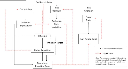
For the estimation of the system, at each iteration the response variables of each of the equations feed another one, in a sequence that enables the simulation and estimation of the system as a whole. The flowchart presented below illustrates the interrelationship of the equations.

Fig 4.2 Flowchart illustrating the interaction of the equations of the system

Among the advantages of the proposed approach in relation to vector autoregressive (VAR) models, the following stand out:

1) The simulation process only requires the variables to be endogenously generated by the model, by ordering a system of equations in which the response variable of one equation feeds the process that will be simulated next. In particular, for example, in the VAR approach it would be impossible to include the variable output gap at time 𝑡 (ℎ𝑡) in equation (4.1), as suggested by the theory;

14 _{Hamilton (1994) recommended using 2 to 5 moments more than the number of parameters estimated, for}

2) It is robust to nonstationarity, so that some of the variables can enter differences into the estimation process without impairing the structural identification of the original model, formulated in level; 3) It is robust to specification, allowing different numbers of lags to be

used in each equation, and each variable of the same equation. Two aspects in common with the VAR method are the possibility of conducting projections and obtaining impulse response functions.

6 Estimates of the Parameters

Next we present the estimates of the equations of the model indicated in section 4, obtained by the method presented in section 515_{, as well as the calculations performed}

to obtain the value of the debt/GDP ratio necessary to put a country in a situation of fiscal vulnerability. In general, logarithmic transformation was applied to the non-negative variables, so the coefficients estimated represent elasticities (except those from equation 4.6, which represent, respectively, semi-elasticity and the coefficient of interaction).

The empirical results presented in this and the following sections should be interpreted with caution. They reflect forecasts about the Brazilian economy. But, of course, only those scenarios that can possibly evolve from the selected model and variables described by equations 4.1 to 4.6.

6.1

To facilitate an exposition of the calculations, the equations estimated are presented together below: 𝜋𝑡= 0.711ℎ𝑡+ 0.496𝑒𝑡+ 0.707(E𝑡𝜋𝑡+1− 𝜋𝑡+1𝑚 ) (6.1) i𝑡= 0.873𝑖𝑡−1+ 1.281(𝐸𝑡𝜋𝑡+1− 𝜋𝑡+1𝑚 ) (6.2) 𝐸𝑡𝜋𝑡+1= 0.623𝜋𝑡−1+ 0.18ℎ𝑡− 0.05ℎ𝑡−1+ 0.24ℎ𝑡−2 (6.3) ℎ𝑡= 0.647E𝑡ℎ𝑡+1− 0.062𝑟𝑡−1− 0.041𝑟𝑡−2− 0.072𝑟𝑡−3 (6.4)

15 _{To simplify, we only report the estimates that are significant at 0.05, except in the case of the coefficients of}

𝐸𝑡−1∆𝑒𝑡= −0.611(i𝑡−1− 𝑖𝑡−1∗ ) + 0.0849𝑟𝑝𝑡 (6.5) 𝑟𝑝𝑡= 237.941 1 + 𝑒−16.91(𝑏𝑡−1−0.803)𝑒 𝑖_{𝑡−1+ 5.624𝑟𝑎} 𝑡−1𝑏𝑡−1 (6.6)

It is important to verify the economic meaning of the results of these equations. According to equation (6.1), the relation between inflation and the output gap is positive. This is logical, since economic expansion tends to increase inflation. The coefficient of exchange rate depreciation in the inflation equation is also positive, which again is expected. The pass-through effect, defined as the elevation of the cost of imported products and inputs when the domestic currency weakens, has a direct impact on inflation.

As modeled by equation (6.2), besides the strong inertial component, the interest rate reacts to the deviation of inflation expectation in relation to the target with elasticity greater than 1. The effect of the output gap, despite being cited often in the minutes of the Monetary Policy Committee (Copom), is not significant at 0.05 (estimate of 0.042, with p-value of 0.17).

Equation (6.3) represents the formation of inflation expectations. In this equation, the effect of the level of economic activity (output gap), according to the proposed specification, is distributed over three months (including the current month) according to the specification (𝑝1= 2). This effect, although significant, has a low magnitude. A

reduction of 1% in the output gap reduces the current value of the inflation expectation for the following month by only 0.18%. This estimate, combined with the effect of the real interest rate on the output gap, will provide the basis for obtaining the effect of monetary policy via aggregate demand in the next section.

Equation (6.4) indicates the influence of the expectation for future economic activity and the lagged real interest rate values (𝑝3= 3) on the output gap.

Equations (6.5) and (6.6) indicate the effect of the interest rate on the risk premium and of that premium on the expectation of currency depreciation. In particular, the impact of the risk premium on the exchange rate is positive, as expected.

6.2

In the rest of this section (including subsections 6.3 and 6.4), we show, by gradually incorporating different components derived from a rise in the basic interest rate, how the proposed model can be used to determine the effects of such a monetary tightening on inflation. The final results of subsection 6.4 will be used as a local approximation to analyze fiscal vulnerability.

Equations (6.1), (6.3) and (6.5) allow the conventional impact of the interest rate on inflation to be obtained by strengthening the exchange rate. The effect of a 1% hike in the Selic rate is obtained by multiplying the coefficient -0.611, which measures the effect of the interest rate on the variation of the exchange rate16 _{in equation (6.5), by}

0.496, to gauge the impact of the exchange rate on inflation in equation (6.1), resulting in −0.611 × 0.496 × 1% = −0.3031%.

Suppose, for example, that the Selic rate rises from 7.0% to 7.5%, an increase of 0.5 percentage points (p.p.), or of 7.14% of the current value17_{. The preceding equations}

suggest an effect on inflation (via the exchange rate) of 7.14% × (−0.3031) = −2.16%. On the other hand, the same increase of 0.5 p.p. in the Selic rate implies, assuming constant inflation of 3%, an increase of 12.5% in the real interest rate. The impact via aggregate demand on inflation observed at 𝑡 would thus be a variation of only 12.5% × (−0.062) × 0.711 + 12.5% × (−0.062) × 0.18 × 0.707 = −0.65%. The first term is the sum of the direct effect, via the output gap, of the increase in the interest rate on inflation (equations 6.1 and 6.4), while the second term denotes the indirect effect, via inflation expectation (equations 6.1, 6.3 and 6.4).

The conclusion is, with respect to the conventional impact of an increase in the interest rate at 𝑡 − 1 on inflation at 𝑡 and under the economic parameters in place up to November 2017, that the effect of the exchange rate predominates over that of aggregate demand (2.16% and 0.65%, respectively).

Therefore, the total conventional impact of an increase of 0.5 p.p. in the interest rate can be obtained by the sum of the influences of the exchange rate and aggregate demand, meaning an effect from 𝑡 − 1 to 𝑡 of −2.16% − 0.65% = −2.81%.

6.3

In the fiscal dominance approach proposed by Blanchard (2005), the risk premium plays a key role as the transmission channel of fiscal problems to the impact of an increase in the interest rate on inflation, possibly even having a reverse effect to that posited by the conventional theory. It is thus essential for our purposes here to identify the conditions under which the effect intermediated by fiscal variables can become dominant.

In this respect, we now calculate the effect of an increase in the interest rate, via the risk premium. Based only on equation (6.5), it can be concluded that to reverse the conventional effect – via covered parity – of an increase of 0.5 p.p. in the interest rate18

16 _{Keeping 𝑖}

𝑡−1

∗ _{constant to simplify.}

17 _{This clarifies the difference between percentage points (p.p.) and percentage variation of the current level in}

the rest of the text.

18 _{Assuming, for simplicity, that i* and 𝐸}

(7.14% if applied to the rate as of this writing, of 7%), an increase greater than (7.14) × (0.611/0.0849)% = 51.38% in the risk premium would be necessary. In fact, assuming an increase of 7.14% in the Selic rate, the variation of the depreciation of the exchange rate, denoted by ∆2_𝑒

𝑡, will be given by:

∆2_𝑒

𝑡= −0.611 × 7.14% + 0.0849∆𝑟𝑝𝑡

Therefore, the variation in the risk premium necessary to offset the interest rate hike, i.e., for ∆2_𝑒

𝑡= 0, will be given by ∆𝑟𝑝𝑡=

0.611∗7.14%

0.0849 = 51.38%.

It should be noted that according to the historical series of the Brazilian component of the EMBI (the variable that represents the risk premium in this paper), during the period studied no variation greater than or equal to 51.38% in the risk premium occurred. The conclusion is that the conventional effect, via the covered parity route, was predominant19_{. Even in the more recent period, during the severe fiscal crisis in}

Brazil, the highest variation observed in the Brazilian EMBI component was 30%, in September 2015. The Central Bank had raised the Selic rate by 0.5 p.p. the month before, and the effect on the risk premium was far from that needed to reverse the effect of that increase on the exchange rate variation.

6.4 Unconventional vs. Conventional effect

In section 6.3 we showed that the conventional impact expected of an increase of 0.5 p.p. in the Selic, through aggregate demand and uncovered parity, considering the parameters estimated with data up to November 2017, would be to reduce inflation by 2.81% in the following month. The next step is to determine as of what debt/GDP ratio value the unconventional effect of this rate increase, as addressed in section 6.3, would dominate the conventional effect, working to increase inflation by more than 2.81% in the ensuing month. Starting at this level, the net result of the higher interest rate will be an increase of inflation.

Based on the estimated equations, it is possible to establish the criterion for the existence of fiscal vulnerability as defined here. The first step is to compute the unconventional effect of monetary policy on inflation, given by the composition, through the simple product, of the effect of an increase of 1 p.p. in the interest rate on the risk premium (given by the coefficient 237.941

1+𝑒−16.91(𝑏𝑡−1−0.803) in equation (6.6),

multiplied by 10020_{) with the effect of the risk premium on the exchange rate (through}

19 _{The last variation of this size in the risk premium (57.8%) happened from May to June 2002 (our study}

period starts in November 2002), in the unsettled period preceding the presidential election.

20 _{In the log-level model, the coefficient needs to be multiplied by 100 to generate the percentage impact on}

the coefficient ˆ₂= 0.0849 in equation (6.5)), and of this on inflation (coefficient ˆ₂ = 0.496 in equation (6.1)).

This effect must be compared with that predicted by the conventional economic theory, composed of three parts. The first part is the exchange rate appreciation resulting from an increase of the interest rate (by means of the coefficient 𝛾̂1= −0.611

in equation (6.5)), and its impact on inflation (coefficient 𝜑̂2= 0.496 in equation

(6.1)). The second and third parts originate from the effect of the interest rate on aggregate demand, represented in the model by the output gap ({β̂𝑗}_𝑗=2

𝑝₂+1

in equation (6.4), equal to -0.062, -0.041 and -0.072, respectively). The output gap, in turn, directly affects inflation (through the coefficient 𝜑̂1= 0.711 in equation (6.1)) as well as the

inflation expectation (via the coefficients {α̂𝑗}_𝑗=1 𝑝1+1

in equation (6.3), equal to 0.18. -0.05 and 0.24, respectively), and through this expectation, actual inflation (by means of the coefficient 𝜑̂3= 0.707 in equation (6.1)).

The comparison of the conventional and unconventional effects described above can provide indications of whether or not the Brazilian economy is under a fiscal vulnerability regime.

We thus consider an increase of 0.5 p.p. in the Selic rate in this section. According to equations (6.1), (6.3), (6.4) and (6.5), the variation of inflation from 𝑡 − 1 to 𝑡 is given by:

∆𝜋𝑡= 0.711 × (−0.062 × 12.5%) + 0.496 × (−0.611 × 7.14%) +

0.707 × [0.18 × (−0.062 × 12.5%)] + 0.496 × 0.0849∆𝑟𝑝𝑡

where ∆𝑟𝑝𝑡 stands for the percent variation of the risk premium.

Note that the first three terms compose the conventional effect, of -2.81%, while the fourth is the unconventional effect. Therefore, to obtain ∆𝜋𝑡= 0, we need

∆𝑟𝑝𝑡= −

(−2.81%)

0.496∗0.0849= 66.73%.

Table 6.1 Effect of an increase of 0.5 p.p. in the Selic rate on inflation

Effect 1 month ahead

Via exchange rate -2.16%

Via aggregate demand -0.65%

Total conventional effect -2.81%

Variation of 𝑟𝑝𝑡 necessary to annul the

conventional effect 66.73%

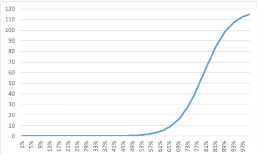
It is interesting to note how the response of the risk premium to the initial elevation of the interest rate depends on the debt/GDP ratio. Figure 6.1 illustrates this point.

Fig. 6.1 Estimated effect of an increase of 0.5 p.p. in the Selic rate on the risk premium (%), considering

different levels of the debt/GDP ratio

0 10 20 30 40 50 60 70 80 90 100 110 120 1% 5% 9% _{13% 17% 21% 25% 29% 33% 37% 41% 45% 49% 53% 57% 61% 65% 69% 73% 77% 81% 85% 89% 93% 97%}

Figure 6.1 shows that the level of 66.7% defined in Table 6.1 is reached for a net debt of about 82% of GDP. Technically, from this point on a fiscal vulnerability regime is configured (since the estimate of the impact necessary for this to occur was 66.73%). The explanation is that starting at a particular debt level, the size of the debt works as a risk alert.

The conclusion is that for fiscal vulnerability to occur, according to the risk premium variation criterion defined in Table 6.1, the consolidated net public sector debt would have to reach 82% of GDP. At the current (2018) debt/GDP ratio, just above 50%21_{, the effect of an interest rate increase on the risk premium, via equation (6.6), is}

only 0.7%.

The final estimates of this table, particularly the elevation of 66.7% in the risk premium necessary for fiscal vulnerability to occur, will serve as a reference for the analyses in the next sections, developed under different scenarios of evolution of the primary surplus.

7 Fiscal Scenarios

To analyze the evolution of inflation and the possible occurrence of fiscal vulnerability, it is necessary to establish hypotheses about the evolution of the fiscal variables.

In scenarios of greater fiscal expansion, the debt/GDP ratio grows faster, increasing the fiscal impact of a desired elevation of the interest rate. This tends to heighten the risk premium, potentially weakening the exchange rate and increasing inflation. In the nomenclature used here, this situation is called fiscal vulnerability.

Scenarios with less fiscal expansion would not have a positive final effect of the increase in the interest rate on inflation because the risk premium would not rise sufficiently. Hence the situation would not be one of fiscal vulnerability.

The analysis conducted is probabilistic, based on stochastic projections of the econometric model estimated for different scenarios of the evolution of government expenditures. Under each of the four scenarios considered below, we obtain the expected path of the debt/GDP ratio and the probability of the occurrence of a fiscal vulnerability regime.

Scenario 1 – evolution of the primary result according to the reaction function used

at present in Brazilian fiscal policy, specified in Campos and Cysne (2018) and updated

21 _{It is important to stress that we only consider the net public sector debt, not the gross debt of the}

below, with the coefficients estimated on the starting date of the projections (November 2017)22_:

s𝑡= 0.023 + 0.943s𝑡−1− 0.016𝑏𝑡−1+ 0.031ℎ𝑡−1+ 0.009𝑃𝑅𝑡 (7.1)

where all the estimates reported are significant at 0.05. Of particular note is the reversal of the sign of the estimate of the fiscal reaction coefficient in relation to that obtained in Campos and Cysne

(2018) for June 2016 (0.032 − 0.016𝑠

).

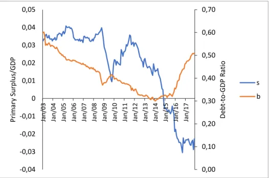
This “negative fiscal reaction” reflects the reversal of the direction of the relation between the primary surplus and the debt (both as percentages of GDP), observed at the end of the sample, as depicted in Figure 7.1 below:

Fig 7.1 Evolution (2003-2017) of the primary surplus and debt (as % of GDP)

In scenarios 2 to 4 below, we consider that revenue, as a percentage of GDP, remains constant over the simulation horizon, with the value in November 2017 taken as a reference.

22 _{In the original work, the function was estimated up to June 2016. Here we updated the estimates to}

November 2017 and the significance of some of the variables, at the 0.05 level, changed.

0,00 0,10 0,20 0,30 0,40 0,50 0,60 0,70 -0,04 -0,03 -0,02 -0,01 0 0,01 0,02 0,03 0,04 0,05 Jan /03 Jan /04 Jan /05 Jan /06 Jan /07 Jan /08 Jan /09 Jan /10 Jan /11 Jan /12 Jan /13 Jan /14 Jan /15 Jan /16 Jan /17 De b t-to -G DP Rat io Prim ar y Su rp lu s/G DP s b

Scenario 2 – growth of government expenditures at the same pace as GDP growth

(considering the projections in November 2017), so that the spending/GDP ratio remains constant, equal to the value observed in November 2017 of 50.99%.

In this scenario, according to the projections used, the spending cap specified by Constitutional Amendment 95/2016 (EC 95/16) is not respected.

Scenario 3 – intermediate between 2 and 4, with expenditures determined as the

simple average of those two scenarios.

Scenario 4 – expenditures as a percentage of GDP declining, as specified in EC

95/16, respecting the corresponding cap, i.e., evolution of expenses limited to inflation (no growth in real terms).

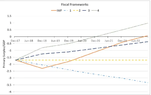
Figure 7.2 below depicts the evolution of the primary surplus in each scenario. We also include, for comparison, the projection prepared by the IMF in its publication

Fiscal Monitor, of April 2018.

Fig 7.2 Evolution of the primary surplus (as % of GDP) under each scenario

The scenario that is closest to the IMF’s projection is scenario 3, which is intermediate between 2 and 4. This similarity is the reason for including that projection.

8 Evaluations of Fiscal Vulnerability

The objective of this section is to demonstrate how the estimation of the model and the estimates of the effects of the interest rate on inflation summarized in Table 6.1 can be used in practice to assess the possibility of fiscal vulnerability (as defined here) in the short and medium terms. For this, as remarked earlier, we consider as references the variation of the risk premium of 66.73% indicated in Table 6.1 and a horizon of five years.

8.

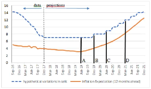
In December 2017 the Selic was 7% a year. The first exercise of this section assumes a simplified context in which the interest rate is maintained at 7% until – as the case may be – inflation rises above the target. As of that point, we assume that the Central Bank implements successive increases until the expectation reacts as envisioned by the conventional theory, returning to the target.

Figure 8.1 below illustrates the average reaction of inflation, obtained by 10,000 simulations of the model, all considering the evolution of expenditures in scenario 1 at the same pace as GDP growth. Note that as of a certain point, fiscal vulnerability occurs due to the continuous elevation of the debt/GDP ratio determined by scenario 1 for the fiscal path. This happens, in this artificial example, when the Central Bank does not change the interest rate in June 2019 (point A in the graph).

Fig. 8.1 Impact of interest rate increases on inflation in scenario

In this exercise, the Central Bank keeps the Selic rate at its initial level of 7% until December 2019, when annual inflation exceeds 4%, the target set for 2019. At that point, the Bank reacts by raising the Selic by 1 p.p. (point B). Nevertheless, inflation continues to rise, providing preliminary indications of the occurrence of fiscal vulnerability.

Six months later, in June 2020, the Central Bank raises the rate by another 1 p.p. (point C), again without success. As of that date, quarterly increases of 1 p.p. are implemented to try to contain inflation, and are still unsuccessful. Indeed, in March 2021 the increase from 11% to 12% appears to accelerate inflation, possibly contributing to increasing its rate of variation.

The explanation for this acceleration is the recurring effect of increasing the interest rate on the debt, which raises the risk premium and weakens the exchange rate, whose impact on inflation is greater than the impact of restricting aggregate demand. Of course, this scenario can be reversed by improving the fiscal scenario.

This exercise, although useful to illustrate the concept of fiscal vulnerability, is unrealistic in two aspects. The first is that it considers the total absence of a fiscal adjustment. The second, more important aspect is that the interest rate was kept constant in the initial period (until December 2019). In this form of the model, the debt path was assumed to be deterministic, reacting to the two exogenous variables (interest rate and spending) according to equation (4.8).

From section 8.2 onward, we relax both conditions, with the intermediate scenarios for public spending, as presented in section 7, and with the market interest rate fluctuating according to the simulated equations.

8.2 Evolution of the debt under each scenario

The average values projected for the debt, under each scenario, are presented below:

Fig. 8.2 Projections of the net debt/GDP ratio under each scenario considered

The line labeled “critical level for fiscal dominance” indicates the point from when, based on the analysis in the preceding section, a situation of fiscal vulnerability would occur, corresponding to a debt/GDP ratio of 82%. In scenario 1 this situation would be reached in the middle of 2021. In the other scenarios, there would be no risk of fiscal vulnerability over the horizon considered. In scenario 4, in particular, the debt/GDP ratio would tend to stabilize, eliminating the possibility of dominance even for longer horizons than considered here.

It should be stressed, however, that this critical level of 82% was obtained by considering the parameters estimated up to November 2017. Each scenario considered for spending, according to the model’s projections, generates different critical values for the debt/GDP ratio. However, in all cases we use the same definition of vulnerability and the variation of the risk premium reported in Table 6.1 (section 6.4).

8.3 Probabilities of fiscal vulnerability according t o the debt/GDP ratio under each scenario

In this section we report the results of simulating and projecting the model 100,000 times, considering each of the scenarios defined in section 7 (total of 500,000 simulations), with an endogenous interest rate evolving according to equation (6.2)23_.

Based on the debt projections and occurrence or not of fiscal vulnerability, we estimated a logistic regression model for each scenario to determine the probability 𝑝𝑖

of occurrence of fiscal vulnerability according to the level 𝑏 of the debt/GDP ratio at which a fiscal vulnerability regime would occur. The model has the following specification:

ln ( 𝑝𝑖 1 − 𝑝𝑖

) = 𝜂0+ 𝜂1𝑏 + 𝑢𝑖 (8.1)

where 𝑝𝑖 = 𝑃(𝑌𝑖 = 1) = 1 − 𝑃(𝑌𝑖 = 0), with 𝑌𝑖 = 1 being, in the i-th simulation,

the relation between the estimated parameters that indicates the existence of fiscal vulnerability, and 𝑌𝑖 = 0 otherwise24. The term 𝜂0+ 𝜂1𝑏 is the linear predictor of the

model and 𝑢𝑖 is a random error term. The expression for the probability of fiscal

vulnerability estimated for a given debt level 𝑏 is obtained directly from equation (8.1) and the estimates of 𝜂0 and 𝜂1, as below:

𝑝𝑖=

1

1 + 𝑒−(𝜂̂₀+𝜂̂₁𝑏) _(8.2)

The probabilities estimated for each scenario according to the debt/GDP ratio, calculated from equation (8.2), are presented in Figure 8.3 below:

23 _{The error term considered in each equation was assumed to be Gaussian, without an}

autocorrelation structure and without a contemporary or lagged correlation with the error terms of the system’s other equations.

24 _{In the cases where vulnerability does not occur over the horizon considered, we}

assumed b to be the value of the debt/GDP ratio reached at the end of the period studied.