Os artigos dos Textos para Discussão da Escola de Economia de São Paulo da Fundação Getulio
Vargas são de inteira responsabilidade dos autores e não refletem necessariamente a opinião da
FGV-EESP. É permitida a reprodução total ou parcial dos artigos, desde que creditada a fonte. Escola de Economia de São Paulo da Fundação Getulio Vargas FGV-EESP
www.eesp.fgv.br Agosto de 2016
Working
Paper
425
Inflation Bias in Latin America
André Sanchez Pacheco
Paulo Tenani
Os artigos dos Textos para Discussão da Escola de Economia de São Paulo da Fundação Getulio
Vargas são de inteira responsabilidade dos autores e não refletem necessariamente a opinião da
FGV-EESP. É permitida a reprodução total ou parcial dos artigos, desde que creditada a fonte. Escola de Economia de São Paulo da Fundação Getulio Vargas FGV-EESP
Inflation Bias in Latin America*
André Sanchez Pacheco¹
New York University and São Paulo School of Economics, FGV
Paulo Tenani²
São Paulo School of Economics, FGV
August 2016
Abstract
This paper accesses the presence of inflation bias in major Latin American Economies over the past decade. Using a small-scale New Keynesian DSGE model and Bayesian Techniques, the time-varying neutral rate of interest is estimated for major Latin American economies. Then the deviations in the policy rate from the neutral rate are overlapped with deviations in current inflation from target. This simple procedure allows the identification of three different regimes of monetary policy – too easy, too restrictive and appropriate. The main result is that Latin American Central Banks often set monetary policy too easy. Analogously, the same conclusion is found if one compares the policy rate with a Taylor Rule-based interest rate aimed at the center of the inflation target range. Such analysis provides evidence of inflation bias in the region, with the exception of Chile.
Keywords: Monetary Policy, Latin America, Neutral Rate, Inflation Bias, DSGE.
* We thank Roberto Cintra and Martin Klos-Rahal for the helpful comments. João Luiz Cesar and João Pedro Cavalcanti provided excellent research assistance.
1. E-mail: asp551@nyu.edu. 2. E-mail: paulo.tenani@fgv.br.
1. Introduction
Policymakers constantly face the temptation of exploiting the short-run Phillips Curve. In any period, the Central Bank may discretionarily set monetary policy as to keep unemployment artificially low by accepting greater inflation in the short run. The problem with this policy is that it will invariably be time inconsistent as indicated by Kydland and Prescott (1977) and will lead to suboptimal results.
Furthermore, Barro and Gordon (1983) showed that this time inconsistent policy will result in an inflation bias equilibrium. If the Central Bank often exploits the Phillips Curve generating unexpected inflation, people will soon understand the policymaker’s true objectives. They will adjust their expectations accordingly by anticipating higher inflation in the future so that these upward surprises don’t occur on a systematic basis. These courses of action will lead to an inefficient equilibrium with excessive inflation.
In this context, Taylor (1993) proposed a simple rule to describe how the monetary authority should set its policy rate. By adopting such rule, the policymaker’s hands are tied and he would not be able to exploit the Phillips Curve. At the same time, the Taylor Rule would ensure that inflation converges to a given target in the relevant horizon of monetary policy.
In practice, several Central Banks adopted the inflation targeting framework during the 1990s with the objective of reducing inflation to targeted low level. According to Bernanke and Mishkin (1997), such strategy is marked by the announcement of official inflation target range and the explicit acknowledgment that low and stable inflation is the overriding goal of monetary policy. According to Wheeler (2015), the goal is to anchor inflation expectations to a desired level. By doing so, whenever economic shocks hit the economy and takes inflation away from the target range, wage and price-setters already expect the Central Bank to act aiming to bring inflation back to target – thus enhancing the monetary policy’s effectiveness.
The adoption of the inflation targeting framework was accompanied by a reduction in inflation rates across the board as shown by Fraga, Minella and Goldfajn (2004) with data until 2002. However, in recent years inflation soared and remained well above target for a long period of time in many Latin American countries. In this context, the goal of this paper is to study whether this persistent increase in inflation can be associated with an inflation bias problem in the region.
The first step is to estimate a small-scale New Keynesian DSGE model that yields the time-varying neutral or natural rate for a group of Latin American countries. In the following analysis both terms are used interchangeably and are defined as the rate that is consistent with zero output gap and stable inflation. This variable will serve as an aggregate to access the stance of monetary policy. If the policy rate is below the neutral nominal rate, then one may infer that monetary policy is easy. Conversely, if the policy rate is above the neutral rate, then one may infer that monetary policy is restrictive.
Before moving forward, it is important to emphasize that the Central Bank does not need to always set the policy rate equal to the neutral rate. In fact, the Central Bank should deviate from the neutral rate whenever inflation is not at the target. Ideally, if inflation is running below target, the Central Bank would like to set the policy rate below its neutral value. Likewise, if inflation is running above target, the monetary authority would choose a policy rate that is greater than the neutral rate.
However, in some circumstances, the Central Bank may - mistakenly or not - set an inappropriate policy rate. For instance, it may set the policy rate below the neutral value at times when inflation is above target. In such scenario, monetary policy is set too easy and it is unlikely to reach its goals. Whether voluntarily or by mistake, the Central Bank is exploiting the Phillips curve. If the monetary authority repeatedly does so, it soon becomes clear for economic agents that the policymakers do have an inflation bias.
Naturally the next step then is to overlap the policy gap – deviations in the policy rate from the neutral nominal rate – with the inflation gap – deviations in inflation from target. This simple procedure also used by Gonçalves (2015) allows one to identify three different regimes of monetary policy – too easy, too restrictive and appropriate.
As explained above, the “too easy” regime is characterized by a negative policy gap and a positive inflation gap. Analogously, the “too restrictive” regime is identified as having a positive policy gap and a negative inflation gap. Lastly the policy gap and the inflation gap have the same sign in the “appropriate regime”.
Using data from 2004 to 2015 for major Latin American Economies, the main conclusion is that the region too often faced “too easy” monetary conditions during the analyzed period. In particular, Brazil have set conditions “too easy” for most of the time (45%) when compared to peers. On the other hand, Chile presents the most balanced result with only 17% of time in “too easy” territory.
The remainder of the paper is structured as follows: Section 2 introduces the model used to estimate the neutral rate among other key variables. The full derivation of the model is shown in Galí (2008). Section 3 describes the data used and the analyzed period and presents the Bayesian Techniques used to properly estimate the model. The results are shown in Section 4. Finally Section 5 presents the conclusion of the article
.
2. The Model
The model used here follows closely the canonical New Keynesian model proposed by Galí (2008). It contains a representative household that lives forever and maximizes its lifetime expected utility, monopolistic firms that produce differentiated goods and maximize profits by using only labor as input and a Central Bank that sets the interest rate according to a monetary policy rule. The model economy also includes price rigidities as in Calvo (1983). Below it will be shown a brief exposition of the key equations that drive the dynamics of this economy. A full derivation of the model can be found in Galí (2008).
Households maximize their lifetime expected utility by choosing how much to consume and work at each period. When solving the household maximization problem, one arrives at the Euler equation that describes the trade-off the individual faces between present consumption and future consumption as a function of the ex-ante real interest rate. If one combines this intertemporal decision made by the representative household with national accounts identity, the result is the Dynamic IS equation:
In which is the output gap defined as where is the current
output and is the natural output to be defined below. is the policy rate and
represents the expected inflation. is the real neutral (or natural) rate of interest determined by:
The Dynamic IS describes the dynamics of the output gap. As it can be seen, there is a negative relationship between expected change in the output gap and deviations in the ex-ante real rate compared to the neutral rate. That is, if the ex-ante real interest rate is equal to the neutral rate then the expected change in the output gap is zero. Using a
similar definition, one can define the nominal neutral rate as .
Also from the household problem one gets the labor supply relationship:
As usual the labor supply condition expresses a positive relationship between labor supplied and real wages. It also indicates that there is a negative relationship between the labor supply and real income.
Now turning to the production side, there is a large number of monopolistic firms that produces differentiated goods using the same technology that takes only labor as input. The aggregate production level of the economy is given by .
In which is the technological level at time t and is the aggregate supply of labor. One can take the logarithm and rewrite the production function as:
Furthermore, the (log of the) technological level is subject a temporary, zero-mean, normally distributed technological shocks that generate the following dynamics:
Next, firms in this economy take both the aggregate price level and consumption as given and maximize the present value of the profit stream by setting prices optimally. However, firms may not be able to reset prices in every period. In fact, it is assumed that at any given periods, firms may reset prices with probability 1-θ which is independent and constant for every firm. Because of this rigidity, whenever firms get the chance to reset prices,
they will do so by considering not only the current economic situation but also expected future conditions as there is a chance it won’t be able to reoptimize prices in the following periods. This feature is crucial for one to derive the New Keynesian Phillips Curve:
In which inflation is defined as .
The New Keynesian Phillips Curve states that current inflation is determined by the output gap and by inflation expectations. In particular, if current output is running above its neutral value (i.e. the output gap is positive), then there will be an upward pressure to current inflation. Likewise, if the output gap is negative, there will be negative pressure to current inflation. Finally, if the individuals expect inflation to be higher in the future, the NKPC suggests the result is that current inflation will be increased today.
Also from the firms’ optimization problem we get to the natural or neutral output that is defined as the level of output that would prevail under flexible prices. It has the following form:
Here note that the natural or neutral output varies over time as it is also subject to productivity shocks.
Lastly, one needs to determine how the nominal interest rate is set in this economy for the model to be complete. In this sense, the Central Bank is assumed to set the nominal interest rate according to a Taylor rule with lag:
That is, the policy rate is a weighted average of the policy rate that prevailed in the previous period and a Taylor rule. Accordingly, the Central Bank reacts to deviations in inflation from target and in current output from natural output.
3. Estimation
The model is estimated using quarterly data ranging from 2004 to 2015 for the following macroeconomic variables: Real GDP growth; inflation; wage growth; employment rate and the policy rate. The group of Latin American countries analyzed here are Brazil, Chile, Mexico and Colombia. The choice of countries was based on their relative size when compared to their regional peers and the fact that these countries have adopted the inflation targeting framework more than 10 years ago. Most of the data used here comes from the national statistical offices and Central Banks. A description of the data used can be found in Appendix A.
To properly estimate the model, some manipulations have to be done with the data. The policy rate and employment rate are expressed in terms of deviations from their means. In addition, the excess inflation used in the model is the difference between the annualized quarterly inflation rate and the target rate. All variables besides the policy rate were seasonally adjusted.
In order to improve the estimation of the model, stochastic shocks , , and are respectively added to equations (I), (VI), (VIII) and (XI). As indicated by Canova (2007), this procedure is not required but it helps reducing the singularity of the covariance matrix of endogenous variables. All five shocks of the model are assumed to be
normally distributed with zero mean and variance .
The estimation of the model is carried out using Bayesian Techniques. According to An and Schorfheide (2007), this estimation method is system-based and fits the solved DSGE model to a vector of time series unlike other methods that are based on equilibrium conditions such as the Generalized Method of Moments. Additionally, this procedure permits the inclusion of prior information in the estimation. This feature is particularly interesting when estimating DSGE models due to the large set of parameters this group of models usually have. In this context, the first step is to assign prior distributions to the parameters of the model. This set of priors is assumed to be the same for all analyzed countries. The mean of these distributions were set around the values proposed by Galí (2008) when studying the
effects of shocks to the model economy. The priors used for the deep parameters of the model are shown in table 1.
TABLE 1 – PRIOR DISTRIBUTIONS
Parameter Distribution (a,b) a b
σ Normal 1.000 0.100 α Normal 0.330 0.020 θ Normal 0.660 0.020 φ_π Normal 1.500 0.100 φ_y Normal 0.125 0.020 ϕ Normal 1.000 0.100 ρ_a Beta 0.600 0.100 β Beta 0.990 0.010 ω Beta 0.400 0.100 σ_a Beta 0.010 0.005 σ_b Beta 0.010 0.005 σ_c Beta 0.100 0.050 σ_d Beta 0.010 0.005 σ_e Beta 0.100 0.050
As in standard Bayesian analysis, the posterior distribution will be proportional to the likelihood multiplied by the prior. Once the priors are defined, the next step is to evaluate the likelihood. Here one potential problem may: If the model has unobserved variables – as it is the case in this paper – then the calculation of the likelihood is not straight-forward. This issue is solved by applying a Kalman Filter as it generates period by period forecasts which allow us to compute the likelihood.
Once one has an estimate of the likelihood, the next step is to sample from the posterior. Since it has no analytical form, one needs to resort to the Metropolis-Hastings algorithm to sample from it as presented by Hastings (1970). This algorithm is a Markov Chain Monte Carlo method that allows one to obtain random samples from probability distributions that don’t have an analytical form.
The procedure works the following way: Consider the set of parameters to be estimated Γ. Choose initial values for that parameter set. Then pass through the Kalman Filter to obtain the likelihood for this set of values . Take also the prior probability
Now generate a candidate set and pass it through the Kalman Filter to obtain the likelihood . Take also the prior probability The Metropolis-Hastings algorithm indicates one should accept with probability α:
If is accepted, then one should set On the other hand, if is rejected then One repeats the procedure by generating a new candidate set and evaluating it against and so on – obtaining a Markov Chain Monte Carlo. This paper uses a random walk to draw candidate sets .
After a large number of repetitions, one needs to check if the Markov Chain converged. This can be done by applying the Brooks and Gelman (1998) test. If the chain converged, the last step is to discard the k first observations as burn-in. The remaining portion of the chain represents a sample from the joint posterior distribution of the parameter set.
In summary, the estimation procedure can be described by the following algorithm: 1. Assign prior distributions to the set of parameters Γ.
2. Choose initial values for the parameter set.
3. Pass through the Kalman Filter to generate an initial estimate of the likelihood. 4. Generate a proposed update using a random walk.
5. Pass through the Kalman Filter to obtain the likelihood for the proposed values.
6. Apply the Metropolis-Hastings test to determine whether to accept or reject the candidate parameter set.
7. Repeat steps 3-6 for a large number of times until the chain converges. 8. Throw out the first k observations.
The model is estimated by using the procedure above for three chains containing 100,000 draws each. The first 20,000 observations are thrown out since one is only interested in drawing from the stable distribution reached once the chain converged.
Once the model is estimated, it is possible to obtain the policy gap by subtracting the neutral nominal rate from the policy rate. Naturally this can be obtained for all four countries.
In addition, it is constructed a Latin American Aggregate as an average of the policy gap for all countries weighted by their relative Gross Domestic Product expressed in Purchasing Power Parity. The composition of the Latin American Aggregate is the following:
TABLE 2 – LATAM AGGREGATE COMPOSITION
Brazil Chile Mexico Colombia Aggregate
2003 49.5% 5.7% 36.2% 8.6% 100.0% 2004 49.8% 5.8% 35.9% 8.6% 100.0% 2005 49.6% 5.9% 35.8% 8.7% 100.0% 2006 49.3% 6.0% 35.9% 8.8% 100.0% 2007 49.8% 6.0% 35.2% 9.0% 100.0% 2008 50.5% 6.0% 34.5% 9.0% 100.0% 2009 51.3% 6.0% 33.4% 9.3% 100.0% 2010 51.9% 6.0% 33.0% 9.1% 100.0% 2011 51.7% 6.1% 33.0% 9.3% 100.0% 2012 51.1% 6.2% 33.3% 9.4% 100.0% 2013 51.3% 6.3% 32.8% 9.6% 100.0% 2014 50.7% 6.3% 33.1% 9.9% 100.0% 2015 49.0% 6.5% 34.2% 10.3% 100.0% Weights
Likewise one can determine the inflation gap as deviations in inflation from target. Here it is also possible to construct a Latin American Aggregate using the same procedure as exposed above.
By overlapping the two time series, one may identify three different regimes of monetary policy – too easy, too restrictive and appropriate. The first one is characterized by a negative policy gap and a positive inflation gap. Analogously, the “too restrictive” regime is identified as having a positive policy gap and a negative inflation gap. Finally the policy gap and the inflation gap have the same sign in the “appropriate regime”.
This simple exercise allows one to draw important conclusions regarding monetary policymaking in the region. The results are shown in the following section.
4. Results
The means of the posterior distribution of parameters can be found in Appendix B. Similarly, the country-specific results can be found in Appendix C. Below it will be shown the results for the Latin American Aggregate.
Figure 1 displays the policy rate and the estimated time-varying neutral nominal rate. The difference between both – that is, the policy gap – was positive until the Global Financial Crisis hit. Latin American Central Banks eased monetary conditions facing adverse external conditions. However, until recently the policy gap had been consistently negative as the neutral nominal rate was greater than the policy rate.
FIGURE 1 – LATAM POLICY RATE AND NEUTRAL NOMINAL RATE
4 6 8 10 12 14 16
LatAm Policy Rate LatAm Neutral Nominal Rate
Note that between 2009 and 2014 the policy rate was set consistently below the Neutral Nominal Rate. This is not enough to say that monetary policy conditions were set “too easy”. In order for one to access the monetary policy stance or regime, it is also necessary to look at the inflation during the period – which will be shown below.
Figure 2 displays the annualized quarterly inflation rate and weighted target rate for Latin American Countries. It can easily be seen that the analyzed period is marked by sequential target misses. Indeed inflation only ran below or at target 16% of the time.
FIGURE 2 – LATAM INFLATION AND INFLATION TARGET
Furthermore, one can see that during 2009 and 2014 – when the policy rate was consistently below the neutral rate – inflation ran above target for most of the time. This result indicates that monetary policy was indeed set “too easy” during the period. Such sequential misses indicates Latin American Central Banks have deliberately explored the Phillips Curve by accepting higher than anticipated inflation in the short-run in exchange for a lower unemployment rate. As previously explained, such policies will inevitably lead to a suboptimal macroeconomic outcome marked by excessive inflation as agents will soon realize the Central Bank’s inflation bias.
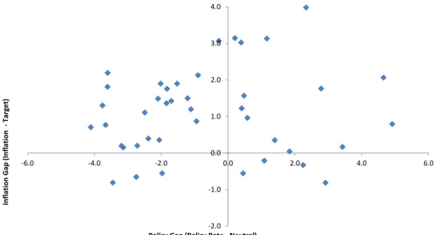
To properly analyze monetary policy stance, it is possible to overlap the policy gap with the inflation gap so one can determine the three monetary policy regimes that can be seen in figure 3. The first and third quadrants indicate monetary policy was appropriate – that is, the inflation was running above (below) target and the policy rate was correctly set above (below) the neutral nominal rate. The second quadrant indicates “too easy” policy. This regime is identified by inflation above target and the policy rate below its neutral value.
Lastly the fourth quadrant indicates “too restrictive” policy regime in which inflation is running above target and the policy rate is set above the neutral rate.
FIGURE 3 – MONETARY POLICY REGIMES IN LATIN AMERICA
-2.0 -1.0 0.0 1.0 2.0 3.0 4.0 -6.0 -4.0 -2.0 0.0 2.0 4.0 6.0 In fl ation Gap (In fl ation -Tar ge t)
Policy Gap (Policy Rate - Neutral)
Note that the largest portion of the data points is located in the third (too easy) quadrant. If a Central Bank does not suffer from inflation bias, then one would expect the monetary policy mistakes – here displayed in the second and fourth quadrants – would be symmetric. This is clearly not the case for Latin America as the distribution of errors is heavily skewed towards “too easy” mistakes.
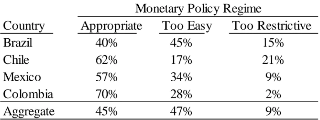
Table 3 summarizes the data points presented in Figure 3. In Latin America, monetary policy was appropriately set for 47% of the time during the analyzed period. Analogously, it was set “too easy” for 45% of the time and “too restrictive” for only 9% of the time. This result shows evidence that, by consistently maintaining an easy monetary policy while inflation was above target, Latin American Central Banks tried to exploit the Phillips Curve.
TABLE 3 – MONETARY POLICY REGIMES IN LATIN AMERICA
Country
Appropriate
Too Easy
Too Restrictive
Brazil
40%
45%
15%
Chile
62%
17%
21%
Mexico
57%
34%
9%
Colombia
70%
28%
2%
Aggregate
45%
47%
9%
Monetary Policy Regime
When analyzing country-specific results, Brazil have set monetary policy “too easy” for 45% of the time. This compares to a mere 9% of the time in “too restrictive” territory. Such imbalanced result suggests the Brazilian Central Bank does suffer from inflation bias. Similar conclusions can be reached for Colombia and Mexico as they also present monetary policy mistakes skewed towards “too easy” monetary policy.
On the other hand, Chile presents a more balance approach as monetary policy mistakes are balanced towards the two directions. This result suggests that deviations from appropriate monetary policy are most likely to come from true mistakes than from deliberate action.
Another interesting result is that on aggregate monetary policy Latin American Countries is set too easy more often than in the countries individually. This is mostly because monetary policy across Latin America is not coordinated – that is, the monetary policy regime one sets does not seem to influence the monetary policy regime of the other country. In fact, monetary policy mistakes seem to be uncorrelated across timing.
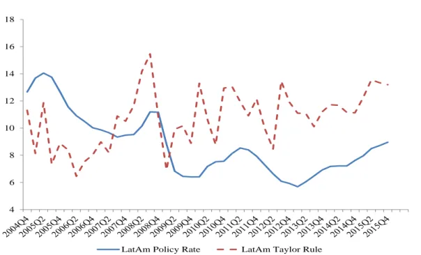
As robustness check, this study also compares the policy rate to a Taylor rule-based rate. The rule specification uses the neutral nominal rate and the reaction coefficients estimated in the DSGE model. Therefore, the posterior mean of the Taylor Rule coefficients are shown in Appendix B. Similarly, the output gap and neutral rate used in the rule are the resulting estimates from the model. Figure 4 shows the policy rate compared to this Taylor rule-based rate.
FIGURE 4 – LATAM POLICY RATE AND TAYLOR RULE 4 6 8 10 12 14 16 18
LatAm Policy Rate LatAm Taylor Rule
As it can be seen, for most of the time the Policy Rate remained below the Taylor rule-based rate. This suggests monetary policy was set “too easy” during the period. In fact, until the Global Financial Crisis hit, monetary policymaking in Latin America did not seem to suffer from inflation bias. In fact, the policy rate was usually set above what a Taylor Rule would recommend. However, the policy rate has been consistently set below the Taylor Rule ever since. This result corroborates the analysis using the policy gap done above as both points towards the existence of inflation bias in Latin America.
5. Conclusion
The evidence presented in this paper indicates that Latin American Central Banks consistently exploit the Phillips Curve, which suggests they have an inflation bias. This is particularly evident post the Great Financial Crisis.
By generating higher-than-anticipated inflation, Central Banks are able to lower the unemployment rate below natural levels in the short-run. Continuous action in the direction of exploiting the Phillips Curve will unequivocally lead – or have already led – to an inefficient equilibrium marked by excessive inflation and deterioration of the credibility of the Central Bank.
As indicated by Blinder (1999), credibility is a key element to determine the costs of disinflation. Taking it to the limit, under certain assumptions, a fully credible Central Bank would be able to reduce inflation without any employment loss. Alternatively, if the Central Bank lacks credibility, the disinflation costs would be higher. In this sense, by constantly exploiting the Phillips Curve, Central Banks in Latin America have eroded their credibility which likely increased the costs of disinflation.
Among the analyzed countries, Mexico, Brazil and Colombia seem to have an inflation bias problem. In particular, Brazil is the most blatant case as monetary policy was inappropriately set “too easy” for most of the time during the analyzed period. This indicates that monetary policy mistakes occur too often in Brazil and are heavily skewed towards “too easy” mistakes.
On the other side, Chile presents no signs of inflation bias as monetary policy mistakes are well-balanced towards the two directions. One possible explanation for this result is that the Chilean Central Bank is more independent than its Latin American counterparts as evidenced by Jácome and Vasquez (2005).
By having greater independence, a Central Bank is less susceptible pressures that push them to fall under the temptation of exploiting the Phillips Curve. In fact, Loungani and Sheets (1995) found that increased central bank independence tends to improve inflation performance. More specifically, countries with independent Central Banks tend to have lower inflation than its counter-parts.
In this sense, one alternative to solve this inflation bias problem in the region would be to increase Central Bank Independence. This would ease pressure on Central Banks to exploit the Phillips Curve and thus to avoid a suboptimal macroeconomic outcome.
References
An, Sungbae and Schorfheide, Frank (2007). “Bayesian Analysis of DSGE Models”. Econometric Reviews, 26(2-4), 113-172.
Barro, Robert J. and Gordon, David B. (1983). “A Positive Theory of Monetary Policy in a Natural Rate Model”. The Journal of Political Economy 91, no. 4, 589-610.
Bernanke, Benjamin S. and Mishkin, Frederic S. (1997). “Inflation Targeting: A New Framework for Monetary Policy?”. NBER Working Paper Series 5893.
Blinder, A. (1999). “Central Bank Credibility: Why Do We Care? How Do We Built It?”. NBER Working Paper 7161.
Brooks, Stephan P. and Gelman, Andrew. (1998) “General Methods for Monitoring Convergence of Iterative Simulations”. Journal of Computation and Graphical Statistics 7, no. 4, 434-455.
Calvo, Guillermo. (1983) “Staggered Prices in a Utility-Maximizing Framework”. Journal of Monetary Economics 12, 383-398.
Canova, Fabio. (2007). Methods for Applied Macroeconomic Research. Princeton University Press.
Fraga, Arminio, Goldfajn, Ilan and Minella, André. (2004). “Inflation Targeting in Emerging Market Economies”. NBER Macroeconomics Annual 2003, no. 18, 365-415.
Galí, Jordi (2008). “Monetary Policy, Inflation and the Business Cycle”. Princeton University Press.
Gonçalves, Carlos E. S. (2015). “Too Tight and Too Loose: Monetary Policy in Brazil”. Working Paper.
Hastings, Wilfried. (1970). “Monte Carlo Sampling Methods Using Markov Chains and Their Applications”. Biometrika 57, no. 1, 97-109.
Kydland, Finn E. and Prescott, Edward C. (1977). “Rules Rather than Discretion: The Inconsistency of Optimal Plans”. The Journal of Political Economy 85, no. 3, 473-492.
Lougani, Prakash and Sheets, Nathan. (1995). “Central Bank Independence, Inflation and Growth in Transition Economies”. Board of Governors of the Federal Reserve System International Finance Discussion Papers 519.
Taylor, John B. (1993). “Discretion versus policy rules in practice”. Carnegie-Rochester Conference Series on Public Policy 39, 195-214.
Wheeler, Graeme (2015). “Reflections on 25 Years of Inflation Targeting Opening Remarks”. International Journal of Central Banking vol. 11 No. S1.
Appendix
A. Data Sources
TABLE 4 – DATA SOURCES
Variable Brazil Chile Colombia Mexico
Gross Domestic Product Instituto Brasileiro de Geografia e
Estatística (IBGE) Banco Central de Chile (BCCH)
Departamento Administrativo Nacional de Estadistica (DANE)
Instituto Nacional de Estadística y Geografía (INEGI) Consumer Price Index Instituto Brasileiro de Geografia e
Estatística (IBGE)
Instituto Nacional de Estadistica
(INE) Banco de la República (BanRep)
Instituto Nacional de Estadística y Geografía (INEGI) Unemployment Rate Instituto Brasileiro de Geografia e
Estatística (IBGE)
Instituto Nacional de Estadistica (INE)
Departamento Administrativo Nacional de Estadistica (DANE)
Instituto Nacional de Estadística y Geografía (INEGI)
Wages Instituto Brasileiro de Geografia e
Estatística (IBGE)
Instituto Nacional de Estadistica (INE)
Departamento Administrativo
Nacional de Estadistica (DANE) Banco De Mexico (Banxico)
Policy Rate Banco Central do Brasil (BCB) Banco Central de Chile (BCCH) Banco de la República (BanRep) Banco De Mexico (Banxico)
GDP PPP World Bank World Bank World Bank World Bank
TABLE 5 – POSTERIOR MEANS
Parameter Prior Mean Brazil Chile Colombia Mexico
σ 1.0000 0.9173 0.3960 0.3683 0.7396 α 0.3300 0.3258 0.3179 0.3293 0.3262 θ 0.6600 0.6601 0.6597 0.6598 0.6601 φ_π 1.5000 1.6420 1.4954 1.5499 1.6255 φ_y 0.1250 0.1235 0.1259 0.1242 0.1216 ϕ 1.0000 1.6420 1.5509 1.3054 1.2780 ρ_a 0.6000 0.6778 0.7899 0.7243 0.8769 β 0.9900 0.9902 0.9900 0.9898 0.9899 ω 0.4000 0.2842 0.3865 0.2561 0.2478 σ_a 0.0100 0.0125 0.0196 0.0081 0.0062 σ_b 0.0100 0.0369 0.0551 0.0601 0.0263 σ_c 0.1000 0.2487 0.4018 0.1206 0.2002 σ_d 0.0100 0.0364 0.0194 0.0215 0.0250 σ_e 0.1000 0.0909 0.0944 0.0892 0.0906 Posterior Mean
C. Country-Specific Results
Brazil
FIGURE 5 – BRAZIL POLICY RATE AND NEUTRAL NOMINAL RATE
6 8 10 12 14 16 18 20 2 0 0 4 Q1 2 0 0 4 Q2 2 0 0 4 Q3 2 0 0 4 Q4 2 0 0 5 Q1 2 0 0 5 Q2 2 0 0 5 Q3 2 0 0 5 Q4 2 0 0 6 Q1 2 0 0 6 Q2 2 0 0 6 Q3 2 0 0 6 Q4 2 0 0 7 Q1 2 0 0 7 Q2 2 0 0 7 Q3 2 0 0 7 Q4 2 0 0 8 Q1 2 0 0 8 Q2 2 0 0 8 Q3 2 0 0 8 Q4 2 0 0 9 Q1 2 0 0 9 Q2 2 0 0 9 Q3 2 0 0 9 Q4 2 0 1 0 Q1 2 0 1 0 Q2 2 0 1 0 Q3 2 0 1 0 Q4 2 0 1 1 Q1 2 0 1 1 Q2 2 0 1 1 Q3 2 0 1 1 Q4 2 0 1 2 Q1 2 0 1 2 Q2 2 0 1 2 Q3 2 0 1 2 Q4 2 0 1 3 Q1 2 0 1 3 Q2 2 0 1 3 Q3 2 0 1 3 Q4 2 0 1 4 Q1 2 0 1 4 Q2 2 0 1 4 Q3 2 0 1 4 Q4 2 0 1 5 Q1 2 0 1 5 Q2 2 0 1 5 Q3 2 0 1 5 Q4
FIGURE 6 – BRAZIL INFLATION AND TARGET RATE 0 2 4 6 8 10 12 2 0 0 4 Q 1 2 0 0 4 Q 2 2 0 0 4 Q 3 2 0 0 4 Q 4 2 0 0 5 Q 1 2 0 0 5 Q 2 2 0 0 5 Q 3 2 0 0 5 Q 4 2 0 0 6 Q 1 2 0 0 6 Q 2 2 0 0 6 Q 3 2 0 0 6 Q4 2 0 0 7 Q 1 2 0 0 7 Q 2 2 0 0 7 Q 3 2 0 0 7 Q 4 2 0 0 8 Q 1 2 0 0 8 Q 2 2 0 0 8 Q 3 2 0 0 8 Q 4 2 0 0 9 Q 1 2 0 0 9 Q 2 2 0 0 9 Q 3 2 0 0 9 Q 4 2 0 1 0 Q 1 2 0 1 0 Q 2 2 0 1 0 Q 3 2 0 1 0 Q 4 2 0 1 1 Q1 2 0 1 1 Q 2 2 0 1 1 Q 3 2 0 1 1 Q 4 2 0 1 2 Q 1 2 0 1 2 Q 2 2 0 1 2 Q 3 2 0 1 2 Q 4 2 0 1 3 Q 1 2 0 1 3 Q 2 2 0 1 3 Q 3 2 0 1 3 Q 4 2 0 1 4 Q 1 2 0 1 4 Q 2 2 0 1 4 Q 3 2 0 1 4 Q 4 2 0 1 5 Q 1 2 0 1 5 Q2 2 0 1 5 Q 3 2 0 1 5 Q 4 Inflation Target
FIGURE 7 – MONETARY POLICY REGIMES IN BRAZIL -4 -2 0 2 4 6 8 -10 -8 -6 -4 -2 0 2 4 6 8 10 Inf lat ion G ap (I nf lat ion -Tar get )
FIGURE 8 – BRAZIL POLICY RATE AND TAYLOR RULE 6 8 10 12 14 16 18 20 22 2 0 0 4 Q1 2 0 0 4 Q2 2 0 0 4 Q3 2 0 0 4 Q4 2 0 0 5 Q1 2 0 0 5 Q2 2 0 0 5 Q3 2 0 0 5 Q4 2 0 0 6 Q1 2 0 0 6 Q2 2 0 0 6 Q3 2 0 0 6 Q4 2 0 0 7 Q1 2 0 0 7 Q2 2 0 0 7 Q3 2 0 0 7 Q4 2 0 0 8 Q1 2 0 0 8 Q2 2 0 0 8 Q3 2 0 0 8 Q4 2 0 0 9 Q1 2 0 0 9 Q2 2 0 0 9 Q3 2 0 0 9 Q4 2 0 1 0 Q1 2 0 1 0 Q2 2 0 1 0 Q3 2 0 1 0 Q4 2 0 1 1 Q1 2 0 1 1 Q2 2 0 1 1 Q3 2 0 1 1 Q4 2 0 1 2 Q1 2 0 1 2 Q2 2 0 1 2 Q3 2 0 1 2 Q4 2 0 1 3 Q1 2 0 1 3 Q2 2 0 1 3 Q3 2 0 1 3 Q4 2 0 1 4 Q1 2 0 1 4 Q2 2 0 1 4 Q3 2 0 1 4 Q4 2 0 1 5 Q1 2 0 1 5 Q2 2 0 1 5 Q3 2 0 1 5 Q4
Policy Rate Taylor Rule
FIGURE 9 – CHILE POLICY RATE AND NEUTRAL NOMINAL RATE 0 1 2 3 4 5 6 7 8 9 2 0 0 4 Q1 2 0 0 4 Q2 2 0 0 4 Q3 2 0 0 4 Q4 2 0 0 5 Q1 2 0 0 5 Q2 2 0 0 5 Q3 2 0 0 5 Q4 2 0 0 6 Q1 2 0 0 6 Q2 2 0 0 6 Q3 2 0 0 6 Q4 2 0 0 7 Q1 2 0 0 7 Q2 2 0 0 7 Q3 2 0 0 7 Q4 2 0 0 8 Q1 2 0 0 8 Q2 2 0 0 8 Q3 2 0 0 8 Q4 2 0 0 9 Q1 2 0 0 9 Q2 2 0 0 9 Q3 2 0 0 9 Q4 2 0 1 0 Q1 2 0 1 0 Q2 2 0 1 0 Q3 2 0 1 0 Q4 2 0 1 1 Q1 2 0 1 1 Q2 2 0 1 1 Q3 2 0 1 1 Q4 2 0 1 2 Q1 2 0 1 2 Q2 2 0 1 2 Q3 2 0 1 2 Q4 2 0 1 3 Q1 2 0 1 3 Q2 2 0 1 3 Q3 2 0 1 3 Q4 2 0 1 4 Q1 2 0 1 4 Q2 2 0 1 4 Q3 2 0 1 4 Q4 2 0 1 5 Q1 2 0 1 5 Q2 2 0 1 5 Q3 2 0 1 5 Q4
FIGURE 10 – CHILE INFLATION AND TARGET RATE -4 -2 0 2 4 6 8 10 12 14 2 0 0 4 Q 1 2 0 0 4 Q 2 2 0 0 4 Q 3 2 0 0 4 Q 4 2 0 0 5 Q 1 2 0 0 5 Q 2 2 0 0 5 Q 3 2 0 0 5 Q 4 2 0 0 6 Q 1 2 0 0 6 Q 2 2 0 0 6 Q 3 2 0 0 6 Q4 2 0 0 7 Q 1 2 0 0 7 Q 2 2 0 0 7 Q 3 2 0 0 7 Q 4 2 0 0 8 Q 1 2 0 0 8 Q 2 2 0 0 8 Q 3 2 0 0 8 Q 4 2 0 0 9 Q 1 2 0 0 9 Q 2 2 0 0 9 Q 3 2 0 0 9 Q 4 2 0 1 0 Q 1 2 0 1 0 Q 2 2 0 1 0 Q 3 2 0 1 0 Q 4 2 0 1 1 Q1 2 0 1 1 Q 2 2 0 1 1 Q 3 2 0 1 1 Q 4 2 0 1 2 Q 1 2 0 1 2 Q 2 2 0 1 2 Q 3 2 0 1 2 Q 4 2 0 1 3 Q 1 2 0 1 3 Q 2 2 0 1 3 Q 3 2 0 1 3 Q 4 2 0 1 4 Q 1 2 0 1 4 Q 2 2 0 1 4 Q 3 2 0 1 4 Q 4 2 0 1 5 Q 1 2 0 1 5 Q2 2 0 1 5 Q 3 2 0 1 5 Q 4 Inflation Target
FIGURE 12 – MONETARY POLICY REGIMES IN CHILE -8 -6 -4 -2 0 2 4 6 8 10 -8 -6 -4 -2 0 2 4 6 8 Inf lat ion G ap (I nf lat ion -Target )
FIGURE 13 – CHILE POLICY RATE AND TAYLOR RULE -4 -2 0 2 4 6 8 10 12 14 16 2 0 0 4 Q1 2 0 0 4 Q2 2 0 0 4 Q3 2 0 0 4 Q4 2 0 0 5 Q1 2 0 0 5 Q2 2 0 0 5 Q3 2 0 0 5 Q4 2 0 0 6 Q1 2 0 0 6 Q2 2 0 0 6 Q3 2 0 0 6 Q4 2 0 0 7 Q1 2 0 0 7 Q2 2 0 0 7 Q3 2 0 0 7 Q4 2 0 0 8 Q1 2 0 0 8 Q2 2 0 0 8 Q3 2 0 0 8 Q4 2 0 0 9 Q1 2 0 0 9 Q2 2 0 0 9 Q3 2 0 0 9 Q4 2 0 1 0 Q1 2 0 1 0 Q2 2 0 1 0 Q3 2 0 1 0 Q4 2 0 1 1 Q1 2 0 1 1 Q2 2 0 1 1 Q3 2 0 1 1 Q4 2 0 1 2 Q1 2 0 1 2 Q2 2 0 1 2 Q3 2 0 1 2 Q4 2 0 1 3 Q1 2 0 1 3 Q2 2 0 1 3 Q3 2 0 1 3 Q4 2 0 1 4 Q1 2 0 1 4 Q2 2 0 1 4 Q3 2 0 1 4 Q4 2 0 1 5 Q1 2 0 1 5 Q2 2 0 1 5 Q3 2 0 1 5 Q4
Colombia
FIGURE 14 – COLOMBIA POLICY RATE AND NEUTRAL NOMINAL RATE
2 3 4 5 6 7 8 9 10 11 2 0 0 4 Q1 2 0 0 4 Q2 2 0 0 4 Q3 2 0 0 4 Q4 2 0 0 5 Q1 2 0 0 5 Q2 2 0 0 5 Q3 2 0 0 5 Q4 2 0 0 6 Q1 2 0 0 6 Q2 2 0 0 6 Q3 2 0 0 6 Q4 2 0 0 7 Q1 2 0 0 7 Q2 2 0 0 7 Q3 2 0 0 7 Q4 2 0 0 8 Q1 2 0 0 8 Q2 2 0 0 8 Q3 2 0 0 8 Q4 2 0 0 9 Q1 2 0 0 9 Q2 2 0 0 9 Q3 2 0 0 9 Q4 2 0 1 0 Q1 2 0 1 0 Q2 2 0 1 0 Q3 2 0 1 0 Q4 2 0 1 1 Q1 2 0 1 1 Q2 2 0 1 1 Q3 2 0 1 1 Q4 2 0 1 2 Q1 2 0 1 2 Q2 2 0 1 2 Q3 2 0 1 2 Q4 2 0 1 3 Q1 2 0 1 3 Q2 2 0 1 3 Q3 2 0 1 3 Q4 2 0 1 4 Q1 2 0 1 4 Q2 2 0 1 4 Q3 2 0 1 4 Q4 2 0 1 5 Q1 2 0 1 5 Q2 2 0 1 5 Q3 2 0 1 5 Q4
FIGURE 15 – COLOMBIA INFLATION AND TARGET RATE 0 1 2 3 4 5 6 7 8 9 10 2 0 0 4 Q 1 2 0 0 4 Q 2 2 0 0 4 Q 3 2 0 0 4 Q 4 2 0 0 5 Q 1 2 0 0 5 Q 2 2 0 0 5 Q 3 2 0 0 5 Q 4 2 0 0 6 Q 1 2 0 0 6 Q 2 2 0 0 6 Q 3 2 0 0 6 Q4 2 0 0 7 Q 1 2 0 0 7 Q 2 2 0 0 7 Q 3 2 0 0 7 Q 4 2 0 0 8 Q 1 2 0 0 8 Q 2 2 0 0 8 Q 3 2 0 0 8 Q 4 2 0 0 9 Q 1 2 0 0 9 Q 2 2 0 0 9 Q 3 2 0 0 9 Q 4 2 0 1 0 Q 1 2 0 1 0 Q 2 2 0 1 0 Q 3 2 0 1 0 Q 4 2 0 1 1 Q1 2 0 1 1 Q 2 2 0 1 1 Q 3 2 0 1 1 Q 4 2 0 1 2 Q 1 2 0 1 2 Q 2 2 0 1 2 Q 3 2 0 1 2 Q 4 2 0 1 3 Q 1 2 0 1 3 Q 2 2 0 1 3 Q 3 2 0 1 3 Q 4 2 0 1 4 Q 1 2 0 1 4 Q 2 2 0 1 4 Q 3 2 0 1 4 Q 4 2 0 1 5 Q 1 2 0 1 5 Q2 2 0 1 5 Q 3 2 0 1 5 Q 4 Inflation Target
FIGURE 16 – MONETARY POLICY REGIMES IN COLOMBIA -4 -2 0 2 4 6 8 -8 -6 -4 -2 0 2 4 6 8 Inf lat ion G ap (I nf lat ion -Target )
FIGURE 17 – COLOMBIA POLICY RATE AND TAYLOR RULE 0 2 4 6 8 10 12 14 16 18 2 0 0 4 Q1 2 0 0 4 Q2 2 0 0 4 Q3 2 0 0 4 Q4 2 0 0 5 Q1 2 0 0 5 Q2 2 0 0 5 Q3 2 0 0 5 Q4 2 0 0 6 Q1 2 0 0 6 Q2 2 0 0 6 Q3 2 0 0 6 Q4 2 0 0 7 Q1 2 0 0 7 Q2 2 0 0 7 Q3 2 0 0 7 Q4 2 0 0 8 Q1 2 0 0 8 Q2 2 0 0 8 Q3 2 0 0 8 Q4 2 0 0 9 Q1 2 0 0 9 Q2 2 0 0 9 Q3 2 0 0 9 Q4 2 0 1 0 Q1 2 0 1 0 Q2 2 0 1 0 Q3 2 0 1 0 Q4 2 0 1 1 Q1 2 0 1 1 Q2 2 0 1 1 Q3 2 0 1 1 Q4 2 0 1 2 Q1 2 0 1 2 Q2 2 0 1 2 Q3 2 0 1 2 Q4 2 0 1 3 Q1 2 0 1 3 Q2 2 0 1 3 Q3 2 0 1 3 Q4 2 0 1 4 Q1 2 0 1 4 Q2 2 0 1 4 Q3 2 0 1 4 Q4 2 0 1 5 Q1 2 0 1 5 Q2 2 0 1 5 Q3 2 0 1 5 Q4
Policy Rate Taylor Rule
FIGURE 18 – MEXICO POLICY RATE AND NEUTRAL NOMINAL RATE 2 3 4 5 6 7 8 9 10 11 2 0 0 4 Q1 2 0 0 4 Q2 2 0 0 4 Q3 2 0 0 4 Q4 2 0 0 5 Q1 2 0 0 5 Q2 2 0 0 5 Q3 2 0 0 5 Q4 2 0 0 6 Q1 2 0 0 6 Q2 2 0 0 6 Q3 2 0 0 6 Q4 2 0 0 7 Q1 2 0 0 7 Q2 2 0 0 7 Q3 2 0 0 7 Q4 2 0 0 8 Q1 2 0 0 8 Q2 2 0 0 8 Q3 2 0 0 8 Q4 2 0 0 9 Q1 2 0 0 9 Q2 2 0 0 9 Q3 2 0 0 9 Q4 2 0 1 0 Q1 2 0 1 0 Q2 2 0 1 0 Q3 2 0 1 0 Q4 2 0 1 1 Q1 2 0 1 1 Q2 2 0 1 1 Q3 2 0 1 1 Q4 2 0 1 2 Q1 2 0 1 2 Q2 2 0 1 2 Q3 2 0 1 2 Q4 2 0 1 3 Q1 2 0 1 3 Q2 2 0 1 3 Q3 2 0 1 3 Q4 2 0 1 4 Q1 2 0 1 4 Q2 2 0 1 4 Q3 2 0 1 4 Q4 2 0 1 5 Q1 2 0 1 5 Q2 2 0 1 5 Q3 2 0 1 5 Q4
FIGURE 19 – MEXICO INFLATION AND TARGET RATE 0 1 2 3 4 5 6 7 8 2 0 0 4 Q 1 2 0 0 4 Q 2 2 0 0 4 Q 3 2 0 0 4 Q4 2 0 0 5 Q 1 2 0 0 5 Q 2 2 0 0 5 Q 3 2 0 0 5 Q 4 2 0 0 6 Q 1 2 0 0 6 Q 2 2 0 0 6 Q 3 2 0 0 6 Q 4 2 0 0 7 Q 1 2 0 0 7 Q 2 2 0 0 7 Q 3 2 0 0 7 Q 4 2 0 0 8 Q 1 2 0 0 8 Q 2 2 0 0 8 Q 3 2 0 0 8 Q 4 2 0 0 9 Q 1 2 0 0 9 Q 2 2 0 0 9 Q 3 2 0 0 9 Q 4 2 0 1 0 Q 1 2 0 1 0 Q 2 2 0 1 0 Q 3 2 0 1 0 Q 4 2 0 1 1 Q 1 2 0 1 1 Q 2 2 0 1 1 Q 3 2 0 1 1 Q 4 2 0 1 2 Q 1 2 0 1 2 Q 2 2 0 1 2 Q 3 2 0 1 2 Q 4 2 0 1 3 Q 1 2 0 1 3 Q 2 2 0 1 3 Q 3 2 0 1 3 Q4 2 0 1 4 Q 1 2 0 1 4 Q 2 2 0 1 4 Q 3 2 0 1 4 Q 4 2 0 1 5 Q 1 2 0 1 5 Q 2 2 0 1 5 Q 3 2 0 1 5 Q 4 Inflation Target
FIGURE 20 – MONETARY POLICY REGIMES IN MEXICO -4 -2 0 2 4 6 -8 -6 -4 -2 0 2 4 6 8 Inf lat ion G ap (I nf lat ion -Target )
FIGURE 21 – MEXICO POLICY RATE AND TAYLOR RULE 0 2 4 6 8 10 12 14 2 0 0 4 Q1 2 0 0 4 Q2 2 0 0 4 Q3 2 0 0 4 Q4 2 0 0 5 Q1 2 0 0 5 Q2 2 0 0 5 Q3 2 0 0 5 Q4 2 0 0 6 Q1 2 0 0 6 Q2 2 0 0 6 Q3 2 0 0 6 Q4 2 0 0 7 Q1 2 0 0 7 Q2 2 0 0 7 Q3 2 0 0 7 Q4 2 0 0 8 Q1 2 0 0 8 Q2 2 0 0 8 Q3 2 0 0 8 Q4 2 0 0 9 Q1 2 0 0 9 Q2 2 0 0 9 Q3 2 0 0 9 Q4 2 0 1 0 Q1 2 0 1 0 Q2 2 0 1 0 Q3 2 0 1 0 Q4 2 0 1 1 Q1 2 0 1 1 Q2 2 0 1 1 Q3 2 0 1 1 Q4 2 0 1 2 Q1 2 0 1 2 Q2 2 0 1 2 Q3 2 0 1 2 Q4 2 0 1 3 Q1 2 0 1 3 Q2 2 0 1 3 Q3 2 0 1 3 Q4 2 0 1 4 Q1 2 0 1 4 Q2 2 0 1 4 Q3 2 0 1 4 Q4 2 0 1 5 Q1 2 0 1 5 Q2 2 0 1 5 Q3 2 0 1 5 Q4