1
A Work Project, presented as part of the requirements for the Award
of a Master Degree in Economics from the NOVA – School of
Business and Economics.
Aggregate and country-specific analysis to
Eurozone Monetary Shock
using a Factor
Augmented VAR approach
Pedro Miguel Formoso da Silva
Student no. 3097
A Project carried out on the Master in Economics Program, under the
supervision of:
Professor Francesco Franco
Professor José Tavares
2
Aggregate and country-specific analysis to Eurozone Monetary Shockusing a
Factor Augmented VAR approach
Abstract
This study aims to analyse the impact of monetary shocks, both on the aggregate euro area as a whole and also at the country level. We estimate a dynamic factor model that summarises the information in a large data set with few estimated factors, subsequently incorporated in a recursive VAR. We find that (i) when compared with the VAR model, the FAVAR better identified the shock, mainly after the 2008 crises; (ii) the monetary policy seems to have lost impact over the economy in recent years; (iii) across countries, the results reveal mixed reactions, being the larger economies the ones that predominantly benefited from the monetary policy.
Keywords: Factor augmented vector autoregressive; Impulse response functions; Eurozone
Monetary Shock; Principal Components.
1. Introduction
The 2010 debt crisis – that followed the 2007/08 financial crisis which considerably affected the developed countries – triggered strong responses from the European Central Bank (ECB) that implemented unconventional policy actions in order to both stabilise prices and bolster economic recovery. Under the existence of a zero lower bound for nominal interest rates, the ECB provided an additional monetary stimulus by applying a large asset purchase policy. Despite long periods of expansionary monetary policy, the persistent low level of inflation combined with the slow recovery of the economy, raised questions on the impacts of ECB policy in the euro area economy, particularly on whether the monetary policy of European Central Bank has benefited some countries in the euro zone more than others.
3
The use of small-scale VAR models with recursive identification schemes in the study of non- systematic monetary policy shock has been employed since Bernanke and Blinder (1992) and Sims (1992). The implementation of this unanticipated component of monetary policy has conducted to reliable empirical responses of macroeconomic variables.
Nevertheless, policy-makers define their monetary policy monitoring a large set of macroeconomic variables from which they extract information. By using a small-scale VAR based on a limited data set, the model suffers an absence of information which might produce inaccurate reactions from the variables, this could signify a reduction of validity of the empirical results, since VAR innovations may not have identified the shock correctly.
Recent empirical macroeconomic literature suggests that, the use of models particularly developed to deal with a large quantity of information generates a better representation of the economic dynamics. Defined as dynamic factor models, they compressed the information embodied in a large quantity of data into a minimal number of factors. The estimation of these models relies in two main methods: principal components and maximum likelihood. Bernanke, Boivin, and Eliasz (2004) found that the maximum likelihood estimation did not offer better results than the principal components method, when assessing the monetary policy impact on the US economy. They also showed preference by the principal component method since it required less burdensome calculations. Regarding the principal components method two main approaches are used to extract the information from the large data set. The first one relies on static principal components for the estimation of factors (Stock and Watson 1998, 1999, 2002a, b) the second is based on dynamic principal components. The former approach was adopted by Ben S. Bernanke, Jean Boivin, Piotr Eliasz (2004), as we follow their seminal work on the estimation of the models, the same methods are computed to build what the authors defined as Factor Augmented VAR (FAVAR) approach. Applying this framework, we reconfirm that the
4
identification of the monetary shock improves with the use of a vast amount of information, as observed in the section where the results of a simple VAR are compared with those of FAVAR.
An important feature of the FAVAR approach is the possibility to analyse the impulse response functions of a large set of variables, improving the study of the subject under discussion. This analysis includes the reactions to the monetary shock on both the aggregate euro area and at a country-specific level. In the first case, a diverse set of 16-time series representing prices, output, exchange rates, monetary aggregates, and employment were observed. On the country-specific level this study examined industrial production, inflation, and real effective exchange rate. The impulse response functions reveal that the ECB´s policy produced the desired impact in the aggregate economy, even if one could say that in the years after the crisis the impact was smaller, with more powerful policies being necessary to achieve the expected results. In the country-specific level, heterogeneous effects were found, with differences regarding the impact of the shock on both the sign and magnitude of the responses to it.
Some studies have already employed a FAVAR approach to evaluate the monetary policy shock at the euro area aggregate level (e.g. Soares (2013). A recent work by Hafemann and Tillmann (2017) studies the reaction from both the aggregate euro area and the specific countries to a monetary shock using instrumental VAR approach. When applicable, the results could be compared to those obtained by these two papers.
The work proceeds as follows: section 2 outlines the methodology for the estimation of a dynamic factor model using principal components. Section 3 addresses the selection and transformations processes of the data. Section 4 displays the empirical analysis of the monetary shock impact in the macroeconomic variables at euro area aggregate level, and country-specific economies.
5
2. Econometric Framework
2.1 Dynamic Factor Models: Dynamic factor models permit to measure the co-movement of
a large set of time series variables. We should distinguish dynamic factor models relatively to the idiosyncratic component of the variables, and the relation among factors and variables. Regarding the former distinction, the model is divided into classical dynamic factor models and the approximate formulation. The classical formulation assumes three restrictive assumptions for the idiosyncratic components: they must be serially and cross-sectional independent as well as uncorrelated with the factors. The approximate formulation allows both, serial and cross-sectional correlation. Some correlation is also allowed between the idiosyncratic component and the factors. Stock and Watson (1998) considered the classical approach inappropriate and found more credibility in using the approximate formulation for the macroeconomic forecasting, since the variables are certainly serially and cross-correlated as, for instance, the monetary aggregates.
The second distinction concerns the static and the dynamic representation of dynamic factor models. On a static specification, the factors have only a contemporaneous effect on the variables since they are incorporated without any lags or leads in the data generating process. Nonetheless, the common factors could incorporate a dynamic process itself, condensing information of a random lag of some fundamental factor.1 Stock and Watson used a static representation in their formulations, where the estimation of the model relied only on the contemporaneous covariances, not capturing any information on the lagging-leading relation of the variables used in the data set.
The dynamic factor model is represented by the vector 𝑋𝑡 of 𝑁𝑥1 stationary and standardised time series variables, observed for time 𝑡 = 1, 2, … . , 𝑇, and defined as a linear combination of
1 In a static representation of a dynamic factor model, all the variables are affected at the same time by the factors, in contrast
6
a small number of factors plus an idiosyncratic component. The latent factors follow a time series process, which is represented commonly as a simple VAR. So, we can express this dynamic model as
(1) 𝑋 𝑡 = 𝜆(𝐿)𝑓𝑡 + 𝑒𝑡
(2) 𝑓𝑡 = Ѱ(𝐿) 𝑓𝑡−1+ 𝑛𝑡
since there are 𝑁 time series, 𝑋 𝑡 and 𝑒𝑡 are 𝑁𝑥1. There are 𝑘 dynamic factors and so 𝑓𝑡 and matrix 𝑛𝑡 are 𝑘𝑥1, 𝐿 is the lag operator. The lag polynomial matrix 𝜆(𝐿) and Ѱ(𝐿) are respectively 𝑁𝑥𝑘 and 𝑘𝑥𝑘. The 𝑖𝑡ℎ lag polynomial 𝜆𝑖(𝐿) is called the dynamic factor loading for the 𝑖𝑡ℎ series, 𝑋𝑡𝑖, and 𝜆𝑖(𝐿)𝑓𝑡 are the common component of the 𝑖𝑡ℎ series. We assume that all the processes in (1) and (2) are stationary.
The model may be expressed in an alternative formulation like:
(3) 𝑋𝑡 = 𝛬𝐹𝑡 + 𝑒𝑡
where 𝐹𝑡 = (𝑓𝑡’, 𝑓𝑡−1’, … , 𝑓𝑡−𝑝’) is 𝑟𝑥1, with a 𝑟 = (𝑝 + 1) 𝑥 𝑘 factors dimension that commands the variables. Loadings are grouped in the 𝑁𝑥𝑟 matrix 𝛬 = (𝜆0, 𝜆1, … . , 𝜆𝑝), where
the 𝑖𝑡ℎ row of 𝛬 = (𝜆
𝑖0, … , 𝜆𝑖𝑝).
The estimation of 𝐹𝑡 is not feasible as the vector of the factors is not identified, considering that
for any invertible 𝑟𝑥𝑟 matrix G, equation (3) can be rewritten as: (4) 𝑋𝑡 = 𝛬𝐺𝐺−1𝐹𝑡+ 𝑒𝑡
where 𝛬𝐺𝐺−1𝐹𝑡 = ₼ 𝑃𝑡 could represent a different set of factors. Note that the 𝑃𝑡 are just a
linear transformation of the factors, so we can compact the information in 𝑋𝑡 using an estimate
of the common factors space, i.e. a r-dimensional orthogonal vector that express the same linear space as 𝐹𝑡.
7
2.2 The principal components: The use of principal components enables the estimation of this
space spanned by the common component and makes use of a nonparametric averaging method. Instead of relying on parametric assumptions, these are made regarding the factor structure. In a nutshell, one must be certain that the factors are pervasive (they affect most or all the series) and that the factor loadings are heterogeneous, meaning that their column values should not be too similar. One must also be assured that the idiosyncratic component has a limited correlation across series. These conditions are set respectively as:
(5) 𝑁−1𝛬’𝛬 → 𝐷𝛬, where 𝐷𝛬has full rank, and (6) 𝑚𝑎𝑥𝑒𝑣𝑎𝑙(Ʃ𝑒) ≤ 𝑐 < ∞ for all 𝑁
where 𝑚𝑎𝑥𝑒𝑣𝑎𝑙 denotes the maximum eigenvalue, Ʃ𝑒 = 𝐸𝑒𝑡𝑒𝑡’,and the limit (5) is taken as 𝑁 → ∞. We can consider the construction of Ft as the weighted cross-sectional average of 𝑋𝑡,2
using a random 𝑁𝑥𝑟 matrix of weights 𝑊, where 𝑊 is normalised such that 𝑊’𝑊/𝑁 = 𝐼𝑟,
(7) 𝐹̂(𝑁−1𝑊) = 𝑁−1𝑊′𝑋𝑡
Replacing (3) into (7):
(8) 𝐹̂(𝑁−1𝑊) = 𝑁−1𝑊′(𝛬𝐹𝑡+ 𝑒𝑡) = 𝑁−1𝑊′𝛬𝐹𝑡+ 𝑁−1𝑊′𝑒𝑡
If 𝑁−1𝑊′𝛬 → 𝐻 when 𝑁 → ∞, where the 𝑟𝑥𝑟 matrix 𝐻 has full rank, and condition (5) and
(6) hold, then 𝐹̂(𝑁−1𝑊) is a consistent estimator of the space spanned by 𝐹
𝑡. Nevertheless,
there are different W that allow a consistent estimation of 𝐹𝑡. Stock and Watson’s approach start with the estimation of 𝛬 and 𝐹𝑡 using principal components, derived as the solution of the
least squared criterion
(9) 𝑚𝑖𝑛𝐹1,…,,𝐹𝑇,𝛬𝑉𝑟(𝛬, 𝐹), 𝑤ℎ𝑒𝑟𝑒 𝑉𝑟(𝛬, 𝐹) = 1
𝑁𝑇∑ (𝑋𝑡− 𝛬𝐹𝑡)′(𝑋𝑡− 𝛬𝐹𝑡) 𝑇
𝑡=1 ,
2 The weak law of large numbers ensures that the expected result from the cross-sectional average of 𝑋
𝑡 is achieved, as the average of the idiosyncratic component will converge to zero remaining only the linear combination of the factors.
8
subject to the normalisation 𝑁−1𝛬′𝛬 = 𝐼𝑟.
Stock and Watson showed that the estimator of 𝐹𝑡 corresponds to the weighted averaging estimator (7) with 𝑊 = 𝛬̂ , where 𝛬̂ represents the matrix of eigenvectors of 𝑋𝑡′𝑠 variance matrix, Ʃ̂𝑋 = 𝑇−1∑𝑇𝑡=1𝑋𝑡𝑋𝑡′. Consequently, 𝐹𝑡 is defined as 𝐹̂(𝑁−1𝑊) = 𝑁−1𝛬̂ 𝑋𝑡,
corresponding to the first 𝑟 scaled principal components of 𝑋𝑡. They also exposed that, when the presumed number of factors is equal to the true number of factors, the estimator 𝐹̂ span the same linear space as 𝐹𝑡.
2.3 FAVAR: Let 𝑌𝑡 be a 𝑀𝑥1 vector representing a set of macroeconomic variables considered
as observed by policy makers. We can simply use these variables to make a VAR or a SVAR, or another multivariate model. Although, as discussed above, to estimate some models we need additional information that could be contained in a small number of factors 𝐹𝑡, represented by
an 𝑘𝑥1 vector of unobservable variables.3
Bernanke, Jean Boivin, Piotr Eliasz (2004) defined the joint dynamics of (𝐹𝑡, 𝑌𝑡) as:
(10) [𝐹𝑡 𝑌𝑡] = ф(𝐿) [ 𝐹𝑡−1 𝑌𝑡−1] + ʋ𝑡⇔ 𝜑(𝐿) [ 𝐹𝑡 𝑌𝑡] = ʋ𝑡
where 𝜑(𝐿) = 𝐼 − ф(𝐿)𝐿 = 𝐼 − ф1𝐿− . . . −ф𝑑𝐿𝑑 is a lag polynomial of finite order d, and ʋ𝑡
is an error with mean zero and covariance matrix 𝑄. When the coefficients that relate 𝐹𝑡 and 𝑌𝑡
are different from zero, the model is designated as Factor Augmented VAR model, FAVAR. The factors are interpreted as common forces that drive the economy, and their number is assumed much smaller than the number of variables in the “informational data set” (𝐾 + 𝑀 < < 𝑁) . We also assume that 𝑋𝑡 are related to the observable variables 𝑌𝑡 and the unobservable variables 𝐹𝑡 by:
3 One should take into consideration that 𝑌
9
(11) 𝑋𝑡= 𝛬𝑓𝐹𝑡+ 𝛬𝑦𝑌𝑡+ 𝑒𝑡
where 𝑒𝑡 is the error terms vector allowed to be cross and serial correlated with zero mean,
𝛬𝑓and 𝛬𝑦 are a 𝑁𝑥𝑘 and 𝑁𝑥𝑀 matrix of factor loadings, respectively. So, as it was analysed in the previous subsection, the informational set, 𝑋𝑡, only depends on the contemporaneous
values of 𝐹𝑡.4
2.4 FAVAR estimation and factors identification: To estimate the FAVAR model (10) and
(11) we will follow the Bernanke, Jean Boivin, Piotr Eliasz’s (2004) approach of two step principal components where the fact that 𝑌𝑡 is observed in the first step is not exploited. The common space spanned by the factors of 𝑋𝑡, i.e. 𝐶(𝐹𝑡, 𝑌𝑡)5 is computed through the 𝑘 + 𝑀 principal components of the “information data set”.6 In the second step, the portion of the common component only related to 𝐹𝑡 must be recovered to obtain 𝐹̂ , thus the part of 𝐶̂(𝐹𝑡 𝑡, 𝑌𝑡) not covered by 𝑌𝑡 shall be removed from the space covered by the principal components, for such procedure an identifying assumption must be established. Since the variables in the information data set react differently to the monetary policy shock, with some variables responding simultaneously and others with delay, a distinction should be done between fast-moving variables (e.g. interest rates) and slow-fast-moving variables (e.g. real variables), respectively. Applying this identification assumption, the “slow-moving” factors are estimated, i.e. 𝐶̂(𝐹𝑡), through the principal components of “slow-moving” variables in the data set.
Regressing the estimated common components 𝐶̂(𝐹𝑡, 𝑌𝑡) on the estimated “slow-moving” factors 𝐶̂(𝐹𝑡) and observable variables, 𝑌𝑡, we obtain:
4 It should be remembered that, some correlation is allowed between 𝑌 𝑡 and 𝐹𝑡 . 5 Bernanke, Jean Boivin, Piotr Eliasz (2004) refer to 𝐶(𝐹
𝑡, 𝑌𝑡) as the common space covered by the factors of Xt which included
both Ft and Yt. Despite being odd to consider also Yt as a factor, the reasoning behind the terminology is that both are
disseminated forces that direct the economy, and, in this way, are considered as common dynamics of all the variables in the informational data set.
6 As explained in the previous section, the computation of the common component 𝐶(𝐹
𝑡, 𝑌𝑡) through principal components
10
(12) 𝐶̂(𝐹𝑡, 𝑌𝑡) = ɑ𝐶̂(𝐹𝑡) + ɓ𝑌𝑡+ 𝑢𝑡
Finally, it is possible to estimate 𝐹𝑡 as 𝐶̂(𝐹𝑡, 𝑌𝑡) − ɓ̂𝑌𝑡. Stock and Watson (2002a) proved that
𝐹̂ can be treated as data for purposes of a second stage least squared regression, and so we use 𝑡 this estimator in equation (10). We can represent this final step as:
(13) 𝜃̂(𝐿) [𝐹̂𝑡
𝑌𝑡] = 𝜀𝑡
where 𝜃̂(𝐿)= 𝜃̂(𝐿)0 − 𝜃̂(𝐿)1𝐿 − . . . − 𝜃̂ (𝐿)𝑑𝐿𝑑 is a matrix of order 𝑑 in the lag operator 𝐿,
𝜃̂(𝐿)𝑗(j=0, 1,…,d) is the coefficient matrix and 𝜀𝑡 is the vector of structural innovations with diagonal covariance matrix. To estimate equation (13) and recover the structural monetary shock, the model is identified by a recursive assumption which assumes that the factors in the model respond with a lag to an unanticipated change on the monetary policy instrument. When we incorporate real variables in the observable vector, 𝑌𝑡 , is also assumed that they react with
a lag to the monetary shock. The recursive identification applies the Cholesky decomposition of the variance-covariance matrix of the estimated residuals. The variable positioned last in the VAR model responds contemporaneously to all the other variables, while the other variables do not respond contemporaneously to this variable ordered last. The reasoning behind the last sentence is applicable to the other variables in the model.
To study how the euro are economy is reacting to the monetary policy, on both country level and as a single aggregated economy is important to observe how a considerably large set of economic variables are reacting to ECB policy. For this reason, impulse response functions of the variables integrated in the vector 𝑋𝑡 could be calculated.
Starting from equation (11), the estimator of 𝑋𝑡 is equal to:
11
Inverting equation (13), we obtain:
(15) [𝐹̂𝑡
𝑌𝑡] = 𝜗̂(𝐿)𝜀𝑡7
where 𝜗̂(𝐿) = [𝜃̂(𝐿)]−1 = 𝜗̂0− 𝜗̂1𝐿 − . . . − 𝜗̂ℎ𝐿ℎ is a matrix of polynomials in order ℎ in the lag operator 𝐿, and 𝜗̂𝑗 (j=0, 1, …, d) is the coefficient matrix. Subsequently, the impulse-response functions can be obtained as follow:
(16) 𝑋𝑡𝐼𝑅𝐹 = [𝛬̂𝑓 𝛬̂𝑦] [𝐹𝑡 ̂ 𝑌𝑡] = [𝛬̂ 𝑓 𝛬̂𝑦]𝜗̂(𝐿)𝜀 𝑡 3. Data
In our application, 𝑋𝑡 consists in a 177 panel of monthly macroeconomic time series, from 2002:01 to 2014:12.8 The data comprises a set of 141 euro area aggregate9 variables complemented by 36 country-specific variables from industrial production, prices and real effective exchange rate. For the country-specific analysis the following countries were selected: Austria, Belgium, Finland, France, Germany, Greece, Ireland, Italy, Luxembourg, the
Netherlands, Portugal, and Spain, that represent for more than 95% of euro area GDP. Since the monetary policy shock is identified by applying a simple recursive assumption that
uses a single variable as the representation of the monetary policy stance, one must select a variable that may reflect the behaviour of monetary policy actions at this period of zero lower bond.10 For this reason, the (shadow) short rate provided by Wu and Xia (2016) 11 was used
7 To compute the transformation in equation 14 it is necessary to ensure the stability condition for the invertibility of the model. 8 The upper limit of the data corresponds to the beginning of quantitative easing by ECB, related to an enlargement of the
unusual measures for the monetary policy. Although, it was estimated a FAVAR model using data between 2008m1 to 2016m12, the differences are discussed in the Empirical Analysis’s section, point 4.4.
9 The set of aggregate variables for the euro area follows the variables selection of Soares (2013) work, although on her work
the aggregate variables used 16 euro area countries from 1999:01 to 2009:03 which is different from the aggregate variables selection in our work that makes use of 19 euro area countries.
10 Previously to the zero lower bound, studies used generally the EONIA rate as representation of the policy instrument. 11 The key ECB interest rates, including EONIA, and the shadow rate are plotted in Figure A.1 on the Appendix A. The shadow
12
between the time available, since 2004/09 onwards. For previous dates we used the EONIA rate.
The data is subjected to four different transformations. Initially, the data is deseasonalized, since seasonality can be so large that masks important characteristics for the purposes of this analysis. In so far as the process is applied over positive series, a multiplicative decomposition method defined as X-12-Autoregressive Integrated Moving Average (X-12-ARIMA) is computed using the Eurostat statistical software, Demetra +. Secondly, a small number of quarterly variables is desegregated into monthly data to be inserted in the data set, using the Eurostat statistical software, Ecotrim. The above-mentioned method considers information from related indicators observed at monthly frequency. An example is the GDP disaggregation that uses the industrial production index as related series.12 The disaggregated process computed by the software is based on the method proposed by Litterman (1983) in which the model estimation is computed in first differences and the regression error corresponds to an Autoregressive AR (1) process.13 The third step is to generate approximate stationary series. Unit root tests are computed in order to establish whether the series are stationary or not. Hence, the series are transformed by first difference or first difference of logarithms.14 Lastly, the data is standardised to take mean zero and unit variance mainly because the different scales of variables could interfere in the factor extraction.
specific time, together with a computed coefficient - that stablish the relations between the shadow rate and the two previous values - results in the short rate value for a specific moment of time.
12 Different types of methods are used to disaggregate the data. There are methods that do not use related series, only comprising
purely mathematical techniques.
13 Litterman (1983) disaggregate method applies first differences to both the explanatory and the dependent variables. Different
types of variables are used as explanatory variables depending on the nature of the dependent variable.
14 The industrial production and harmonised index of consumer prices incorporated initially in the simple-VAR model are
13
4. Empirical Analysis
4.1 Empirical Implementation: Starting with a simple 3 variable small-scale VAR, we
selected the log of industrial production, the log of harmonised index of consumer prices as well as the policy instrument. The model is identified by Cholesky decomposition using the previous order in a standard way, where the interest rate does not affect contemporaneously the industrial production and prices, although it is defined by the ECB considering the contemporaneous value of the two other variables. Based on this simple formulation, the factors are included in the model, resulting in a FAVAR structure. All models are defined with 3 lags, that emerge from the computation of common likelihood tests,15 nevertheless, if we increase the number of lags until 6 the results are fairly similar. The selection of the number of factors to extract from the data set is based upon the common Information Criterion IC2(k) by Bai and
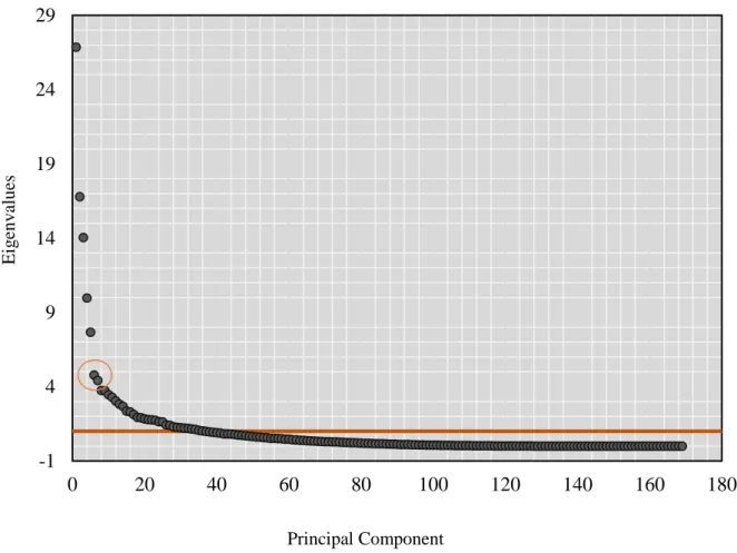
Ng (2002). However, one can also deduce the number to extract simply by observing the eigenvalues for the principal components of the information data set.16
Albeit providing the information on the number of factors to extract from the data, the common Information Criterion IC2(k) by Bai and Ng (2002) does not provide with the knowledge
concerning the number of factors to introduce in the VAR. In order to test the number of factors to introduce in the model we use a specification with 6 factors and conclude that adding up a larger number factors does not change the results significantly.
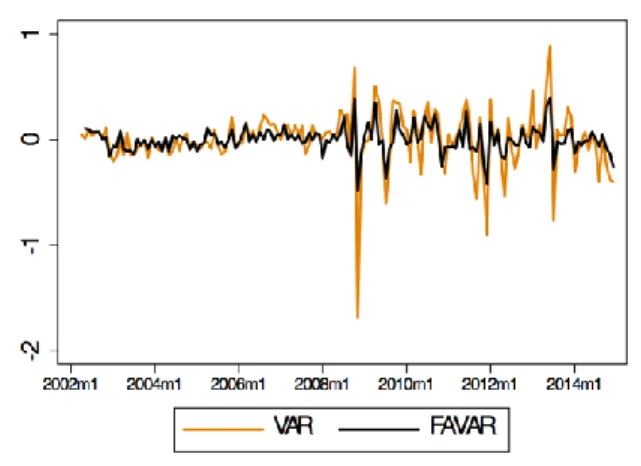
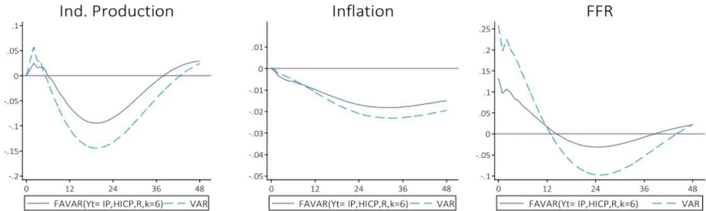
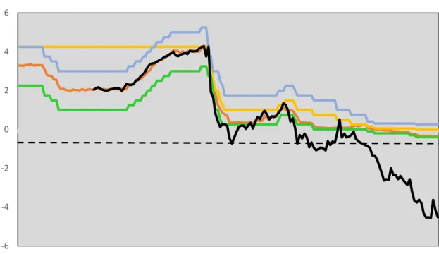
4.2 Comparing VAR and FAVAR: Figure 1 and 2 represent the monetary policy shock for
the VAR and Baseline FAVAR (the specification with 6 Factors) models and the impulse response function of industrial production (IP), inflation (HICP) and interest rate (R) to the monetary policy shock, respectively. Since the monetary shock in analysis is defined as the
15 As common tests we are referring to: Akaike’s information criterion (AIC), Schwarz’s Bayesian information criterion
(SBIC), and the Hannan and Quinn information criterion (HQIC).
16 The Figure A.2 in the Appendix A shows the eigenvalues for the principal components of the informational data set,
14
unexplained changes of our policy instrument, the expectation when the information inside the model increases is that a better representation of the policy behaviour could be achieved, which reduces the variance of the shock. Until 2008, the shock in the VAR model was very similar to the baseline FAVAR, so increasing with factors does not appear to be of significant relevance. After the 2008 crisis, the variance of the shock increased considerably in both models, which may be explained by a more unpredictability of the ECB’s policies. However, in the VAR model, the variance increases significantly more
when compared with the FAVAR.
Consequently, the latter seems to capture important information upon which the ECB’s policy action is based, which certainly entails the more accurate identification of the monetary policy shock. Regarding Figure 2, the behaviour of the variables matches, in both models, the expected movements after a tightening of the monetary policy. In fact, the VAR model’s responses are better than expected. It is common to observe a “price puzzle”17 on the response of inflation when a standard Cholesky identification is used on a small-scale VAR model, however one can say that its reaction corresponds to the expected one, with constant decrease until it stabilises on a lower level. Industrial production has the characteristic U-shape curve, reacting negatively to the monetary contraction but returning towards zero while the effect of the shock fades way.
The short run interest rate response is as well in line with the theoretical arguments, initially reacting to their own shock and then fading out until returning to the baseline.
17 Price puzzle is a counterintuitive movement of prices in the short run caused by an information lack in the model. In the case
of a contractionary policy, prices increased in the first few periods, dropping then below the baseline level.
Fig. 1: Time series representation of the shocks for the
baseline FAVAR (Yt = IP, HICP, R; k=6) and small-scale VAR model (IP, HICP and R), identified by Cholesky.
15
Despite the fact that the responses in both models reproduce the expected movements, we can also observe that the FAVAR model presents indeed more suitable responses than the VAR, mainly in the industrial production and interest rate. The seen reactions in the first model, in the medium term, do not exhibit such an abrupt descent as they did in the latter, which seems more reasonable. In both models the industrial production achieves its maximum 19 months after the shock, although it only changes - 0.09 percentage points in the FAVAR model whereas in the VAR it reaches -0.15 percentage points. To complete the analysis, Table 1 indicates the standard deviations for the 3 impulse response functions, where the VAR specification has the lowest precision for all the three variables with the main difference occurring in the interest rate variable. This steady behaviour and more precision of the impulse response functions are related to a better identification of the monetary policy shock due to the use of more information throughout the introduction of factors.
Fig. 2: Impulse responses to a contractionary policy shock. All the deviations from the baseline(represented in the y-axis)
are in percentage points. In the abcissa are the months following the monetary policy shock. Note: The monetary shock was standardized to reflect a 25-basis-point innovation in the ECB policy instrument.
Table 1: Uncertainty of Impulse response functions. Standard errors, computed using a standard bootstrap with 500
iterations, for the responses to the monetary policy tightening shock. Numbers in bold display the highest values between the two formulations.
Inflation Ind. Production Interest Rate
Baseline FAVAR 0.00545 0.047 0.0379 VAR 0.00772 0.0638 0.09097 Table 1 -.2 -.15 -.1 -.05 0 .05 .1 0 12 24 36 48
FAVAR(Yt= IP,HICP,R,k=6) VAR Ind. Production -.05 -.04 -.03 -.02 -.01 0 .01 0 12 24 36 48
FAVAR(Yt= IP,HICP,R,k=6) VAR Inflation -.1 -.05 0 .05 .1 .15 .2 .25 0 12 24 36 48
FAVAR(Yt= IP,HICP,R,k=6) VAR FFR
16
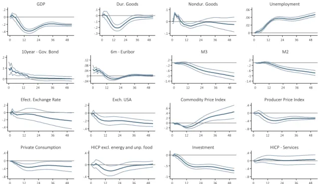
4.2 The euro area aggregate level analysis: Together with the better identification of the
shock, an important reason for the use of a FAVAR is that it allows the conclusions to be drawn from the analysis of a large set of variables.
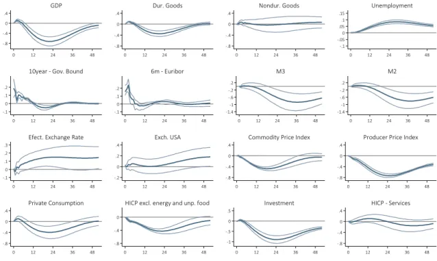
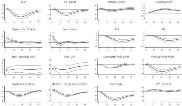
Making full use of equation (16) we computed the impulse response functions to a negative monetary policy shock, standardised to correspond to 0.25 basis-point innovation in the policy instrument, of 16 variables whose nature is related with prices, output, interest rates, unemployment, exchange rates, and monetary aggregates for the euro area economy, which are represented in Figures 3 and 4. 18 Figure 3 represents the responses in our baseline FAVAR that uses 6 factors, in Figure 4 displays the responses for the FAVAR computed with 3 factors.
Regarding Figures 3 and 4, most of the impulse response functions have an intuitive shape and sign. Even though a few number of variables hold an unexpected behaviour between 2002:01 to 2014:12, when observed from an aggregate point of view, that does not disrupt the fact that the ECB’s monetary policy leads to standard reactions in the euro area economy. Comparing both figures, one cannot identify significant differences between the responses, although the baseline FAVAR with 6 factors improves some anomalies in the reactions such as the GDP responses and the effective exchange rate reaction, being this reaction the less standardised. An unexpected contraction of the monetary policy leads to a regular decrease in GDP, reaching the maximum effect around 20 months, as the industrial production which is observed in Figure 2. Nonetheless, the magnitude of both cannot be compared inasmuch as the response of industrial production is measured in percentage points whereas the GDP response is measured in percentage. The maximum response of GDP stays between -0.7% and -0.8%. When the number of factors in the model increases, the GDP returns to the baseline faster and there is no persistent
18 Even though only a small subset of variables is displayed, it must be noted that it is feasible to achieve the impulse response
for all the variables in 𝑋𝑡, since any variable in the panel could be represented by a linear combination of 𝑌𝑡 and 𝐹̂ plus an 𝑡
17
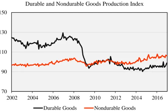
negative behaviour in the long run, which happens when only 3 factors are added to the VAR. Dividing the industrial production into durable consumption goods and nondurable consumption goods, the results point to a distinct reaction of each group. The former has a similar reaction to the monetary shock as GDP, reaching the maximum impact near 20 months after the shock, although the maximum magnitude is smaller, achieving -0.4%, in the baseline model. The impact on the non-durable consumer goods is null. Two different aspects could be causing this effect, first the development of the nondurable goods was less dramatic during the 2008 crisis even though its behaviour has been in line with overall industrial production.19 Secondly – and this aspect is connected to the nature of the products – since nondurable goods are typically less expensive and could be purchased without applying for credit the impact of the monetary policy shock on interest rates and credit facilities does not affect substantially their demand. After the monetary shock, one may say that in some degree, it could exist a
19 The Index of Durable, and Nondurable Goods are shown in Figure A.3 of Appendix.
-.8 -.4 0 .4 0 12 24 36 48 GDP -.8 -.4 0 .4 0 12 24 36 48 Dur. Goods -.8 -.4 0 .4 0 12 24 36 48 Nondur. Goods -.1 -.05 0 .05 .1 .15 0 12 24 36 48 Unemployment -.1 0 .1 .2 0 12 24 36 48
10year - Gov. Bound
-.1 0 .1 .2 0 12 24 36 48 6m - Euribor -1.4 -1 -.6 -.2 .2 0 12 24 36 48 M3 -1.4 -1 -.6 -.2 .2 0 12 24 36 48 M2 -.1 0 .1 .2 .3 0 12 24 36 48
Efect. Exchange Rate
-.2 0 .2 .4 0 12 24 36 48 Exch. USA -.8 -.4 0 .4 0 12 24 36 48
Commodity Price Index
-.8 -.4 0 .4
0 12 24 36 48
Producer Price Index
-.8 -.4 0 .4 0 12 24 36 48 Private Consumption -.8 -.4 0 0 12 24 36 48
HICP excl. energy and unp. food
-1 -.5 0 .5 0 12 24 36 48 Investment -.8 -.4 0 .4 0 12 24 36 48 HICP - Services
Fig. 3: Impulse response function to a contractionary shock for the Baseline FAVAR (Yt = Policy Instrument, Industrial Production, Prices; six factors k=6). In the ordinates are represented the deviations from the origin in percentage (%) – for
all the variables – except the interest rates which are percentage point deviations. In the abcissa are the number of months after the monetary policy shock. The confidence bands delimited an 90% confidence level.
18
positive effect in the productioncreated by a substitution effect between both types of goods. In the FAVAR with 3 factors the substitution effect appears to be more relevant, since the impulse response is above zero in the long run.
Private consumption and investment also reflect the expected reaction to the shock. Consumption suffers from a higher short-term interest rate that leads to a more expensive financing, with the maximum negative impact of -0.4% reached 20 months after the shock. In the investment expenditure, increasing the cost of the money decreases the return rate of investment which causes a persistent effect with a large maximum magnitude of -1.0% around 2 years after the shock. Hence, an increment in the interest rates generates a more considerable negative response on investment than it does on the consumption.
The producer price index has a similar reaction to the overall inflation, with a permanent negative effect. The different disaggregated components of prices have distinct responses to the monetary policy shock. Boivin et al. (2009) concluded that, when disaggregated analysed prices
-.8 -.4 0 .4 0 12 24 36 48 GDP -.8 -.4 0 .4 0 12 24 36 48 Dur. Goods -.8 -.4 0 .4 0 12 24 36 48 Nondur. Goods -.1 -.05 0 .05 .1 .15 0 12 24 36 48 Unemployment -.1 0 .1 .2 0 12 24 36 48
10year - Gov. Bound
-.1 0 .1 .2 0 12 24 36 48 6m - Euribor -1.4 -1 -.6 -.2 .2 0 12 24 36 48 M3 -1.4 -1 -.6 -.2 .2 0 12 24 36 48 M2 -.1 0 .1 .2 .3 0 12 24 36 48
Efect. Exchange Rate
-.2 0 .2 .4 0 12 24 36 48 Exch. USA -.8 -.4 0 .4 0 12 24 36 48
Commodity Price Index
-.8 -.4 0 .4
0 12 24 36 48
Producer Price Index
-.8 -.4 0 .4 0 12 24 36 48 Private Consumption -.8 -.4 0 0 12 24 36 48
HICP excl. energy and unp. food
-1 -.5 0 .5 0 12 24 36 48 Investment -.8 -.4 0 .4 0 12 24 36 48 HICP - Services
Fig. 4: Impulse response function to a contractionary shock for the FAVAR (Yt = Policy Instrument, Industrial Production, Prices; six factors k=3). In the ordinates are represented the deviations from the origin in percentage (%) – for
all the variables – except the interest rates which are percentage point deviations. In the abcissa are the number of months after the monetary policy shock. The confidence bands delimited an 90% confidence level.
19
are more volatile than is assumed in studies based on aggregate data. In fact, observing the reactions of prices, the results are in consonance with Boivin. Commodity prices returns to the baseline after a decrease. Prices excluding unprocessed food and energy also return to the baseline. In the services, for the baseline model, the reaction is null at the 90% significance level.
The monetary aggregates stay in the baseline during almost a 14-months span decreasing then constantly until two and a half years where they remain below the baseline level. In the long-run, the reductions in monetary aggregates will reflect the increase of refinancing costs due to the raise of interest rates, which leads to a small demand for credit.
The unemployment response shows the existence of two economic events, that are reflected normally in the labour market: hysteresis and the existence of wage rigidities. Regarding the former, the persistence of the shock in the long-run is related to social reasons, such as an adjustment of living standards when unemployment increases or a greater social acceptance to be unemployed when the number of unemployed workers is considerable, which could lead to the indifference by some jobless to return to the work force when labour market returns to normal. It is also related to the automatisation in the labour market that makes workers’ skills to became obsolete which hinders them from reentering in the job market. The rigidity of nominal wages, by not allowing adjustments in their levels after prices drop, increases real wages, continuously impacting on unemployment in the long run. In Hafemann and Tillmann (2017), a persistent effect on unemployment is also achieved, even when industrial production reacts normally.
Both interest rates follow the policy short-term interest rate closely, with the Euribor recovering faster from the shock and returning to the baseline level sooner than the 10-year government bound.
20
The nominal effective exchange rate, as well as the exchange rate of US dollar have no effect in the FAVAR using 3 factors. Although, when the number of factors introduced in our model increased, the results improved, with the sign of the nominal effective exchange rate response becoming positive. The economic logic behind the reactions of the variables is that, a higher interest rate invites for more investment and leads to capital inflows causing the appreciation of the euro. The problem observed, mainly in our FAVAR with only 3 factors is the difficulty in capturing the reaction of the ECB as a policy-maker of an open economy, which takes into account the actions of foreign monetary authorities and expected inflation in those countries in order to define its own policy. The information conveyed by the additional factors introduced in the baseline FAVAR may be related to the improved reaction of the nominal effective exchange rates, which appears to have the expected movement, with an appreciation followed by a return to the baseline level, not violating the uncovered interest parity, nonetheless, we should interpret these results with caution. In Soares (2013) the impact in the nominal effective exchange rate is always counterintuitive for all model specifications.
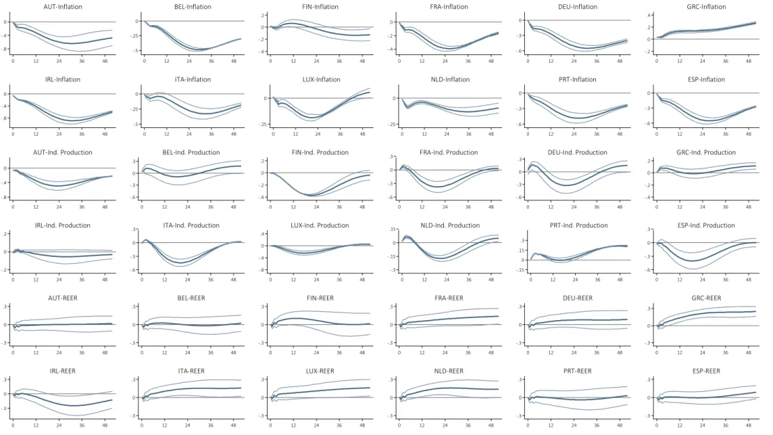
4.3 Country-specific level analysis: Figure 5 shows all the impulse response functions for
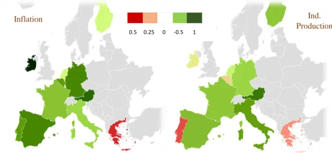
industrial production, harmonised index of consumer prices and real effective exchange rate of each country, also employing equation (16). Figure 6 summarises the maximum response of industrial production and inflation across the different countries in an intuitive way, assisting in the interpretation of the results. The real effective exchange rate responses are not significant in most countries, therefore the analysis will focus mainly on the industrial production and inflation.
In nearly all the euro area countries, industrial production decreases in the short-run returning to the baseline level in the medium term as expected. However, the magnitude of the responses varies considerably across them. Austria has the largest reaction to the monetary shock reaching -0.61% after 2 years and keeping a small persistent effect in the long-run. Followed, by this
21 -.8 -.4 0 0 12 24 36 48 AUT-Inflation -.5 -.25 0 0 12 24 36 48 BEL-Inflation -.4 -.2 0 .2 0 12 24 36 48 FIN-Inflation -.4 -.2 0 0 12 24 36 48 FRA-Inflation -.6 -.3 0 0 12 24 36 48 DEU-Inflation -.2 0 .2 .4 0 12 24 36 48 GRC-Inflation -.8 -.4 0 0 12 24 36 48 IRL-Inflation -.5 -.25 0 0 12 24 36 48 ITA-Inflation -.25 0 0 12 24 36 48 LUX-Inflation -.25 0 0 12 24 36 48 NLD-Inflation -.6 -.3 0 0 12 24 36 48 PRT-Inflation -.6 -.3 0 0 12 24 36 48 ESP-Inflation -.8 -.4 0 0 12 24 36 48 AUT-Ind. Production -.6 -.3 0 .3 0 12 24 36 48 BEL-Ind. Production -.4 -.2 0 .2 0 12 24 36 48 FIN-Ind. Production -.6 -.3 0 .3 0 12 24 36 48 FRA-Ind. Production -.6 -.3 0 .3 0 12 24 36 48 DEU-Ind. Production -.4 -.2 0 .2 0 12 24 36 48 GRC-Ind. Production -.2 0 .2 0 12 24 36 48 IRL-Ind. Production -.6 -.3 0 .3 0 12 24 36 48 ITA-Ind. Production -.8 -.4 0 .4 0 12 24 36 48 LUX-Ind. Production -.3 -.15 0 .15 0 12 24 36 48 NLD-Ind. Production -.15 0 .15 .3 0 12 24 36 48 PRT-Ind. Production -.6 -.3 0 .3 0 12 24 36 48 ESP-Ind. Production -.3 0 .3 0 12 24 36 48 AUT-REER -.3 0 .3 0 12 24 36 48 BEL-REER -.3 0 .3 0 12 24 36 48 FIN-REER -.3 0 .3 0 12 24 36 48 FRA-REER -.3 0 .3 0 12 24 36 48 DEU-REER -.3 0 .3 0 12 24 36 48 GRC-REER -.3 0 .3 0 12 24 36 48 IRL-REER -.3 0 .3 0 12 24 36 48 ITA-REER -.3 0 .3 0 12 24 36 48 LUX-REER -.3 0 .3 0 12 24 36 48 NLD-REER -.3 0 .3 0 12 24 36 48 PRT-REER -.3 0 .3 0 12 24 36 48 ESP-REER
Fig. 5: Impulse response function of IP, HICP, and REER for each of the 12 countries to a contractionary shock for the Baseline FAVAR (Yt = Interest Rate, Industrial Production, Prices; six factors k=6). In the ordinates are the deviations from the origin in percentage (%). It should be noted that y-scale could be different even when considered for the same variables, to allow a better
22
order, by Italy, Spain, Finland, France, and Germany, all with a maximum impact near -0.5%. However, contrary to Austria, they return to the baseline level in the long-run. Portugal and Greece have an inverse reaction to the monetary policy shock in this period, being Portugal more affected than Greece with an impact of 0.2% against 0.14%. The remaining countries have a standard reaction to the shock, even though – when compared with the first group of countries listed – the impact is smaller, in some cases close to zero, as easily observed in Figures 6. Price’s responses have the theoretical expected behaviour in all countries in the data set except Greece and Luxembourg, the former has an inverse reaction and the latter does not have a persistent response over inflation in the long-run. Again, what emerges in the price’s response is the heterogeneous intensity on the shock’s impact. Ireland and Austria have the largest reaction, around -0.9% and -0.65%, respectively. They are followed by Spain, Germany, Belgium, Portugal, France, and Italy. The remaining countries have a residual maximum response.
Overall, the responses across countries are heterogeneous mainly in the magnitude of the impact in all the variables presented. Even in REER the few significant results are different and in some cases with opposite signs.
0.5 0.25 0 -0.5 1
Inflation Ind.
Production
Fig. 6: In the maps are represented the maximum impact of the response function to the monetary policy shock.
When the county is painted green the reaction has the expected sign, painted red has the opposite sign. More intense colour means stronger impacts, the faded colours represent responses close to zero.
23
The larger economies as Germany, France, Italy, Spain are affected in the expected away. Austria, Ireland, Belgium, the Netherlands, and Finland have more extreme responses to at least one of the variables. Ireland and Austria seem to be heavily affected in prices, whereas Finland, the Netherlands, and Luxembourg have nearly a null response. In terms of production, there is a persistent effect in Austria and almost no response by the Netherlands, Luxembourg, Ireland, and Belgium. Portugal, in terms of production, and Greece in inflation and production are more negatively affected, since the monetary shocks disturbed them in a counterintuitive way.
4.4 Confronting section 4.2 with estimations employing data from 2008:01 to 2016:12:
Regarding Figure 7, the results of the impulse response functions for these years of economic and financial crisis are different than the results analysed in the 4.2 subsection.
Currently, the behaviour of the effective exchange rate and USD exchange rate have become counterintuitive, probably for the reasons presented above, even when computed with the corrected specifications of the model for this data set, using 7 factors. In broader terms, the reactions to the monetary policy shock have now a more persistent effect on the real variables like investment expenditure, unemployment, and GDP and a smaller impact over the economy in general. The investment seems to remain in a negative or stable trajectory below the baseline level, never recovering for the maximum negative impact of the monetary policy shock. For almost all the variables, excluding the monetary aggregates, the magnitude of the response is smaller than before. The above-mentioned scenario has conducted, in recent years, the monetary policy shock to have less marginal impact over the variables, mainly in prices that are now less responsive to the ECB policies. The impact of the monetary policies is dependent on some factors that are not under the control of the ECB, just as the confidence of consumers and investors. In a period of crisis, when there is a credit crunch, even if the ECB is cutting on interest rates, this does not substantially change the fact that banks are not able to provide credit.
24
Therefore, the ECB has regarded as necessary to implement extreme monetary policies. Even if there is a higher risk of not controlling their impact on the economy, or even if they entail a possibility of not producing any results, in contrast with the measures applied in previous periods.
6.
Conclusion
The monetary policy effects in the euro area were the focus of this study – both based on aggregate and country-specific data. Since policy makers consider a large amount of data, a dynamic factor model was computed – currently a cornerstone of macroeconometric modelling – that summarises the information in a large data set with few estimated factors, then incorporated in a recursive VAR.
When compared with a simple recursive VAR, the FAVAR model provided for a more complete identification of the monetary policy shock, especially in the period after the 2008
-.4 -.2 0 .2 0 12 24 36 48 GDP -.3 -.2 -.1 0 .1 0 12 24 36 48 Dur. Goods -.1 0 .1 0 12 24 36 48 Nondur. Goods 0 .02 .04 .06 0 12 24 36 48 Unemployment 0 .1 .2 0 12 24 36 48
10year - Gov. Bond
-.04 0 .04 .08 .12 0 12 24 36 48 6m - Euribor -1.4 -1 -.6 -.2 .2 0 12 24 36 48 M3 -1.4 -1 -.6 -.2 .2 0 12 24 36 48 M2 -.4 -.2 0 .2 0 12 24 36 48
Efect. Exchange Rate
-.4 -.2 0 .2 0 12 24 36 48 Exch. USA -.2 0 .2 .4 .6 0 12 24 36 48
Commodity Price Index
-.8 -.4 0 .4
0 12 24 36 48
Producer Price Index
-.8 -.4 0 .4 0 12 24 36 48 Private Consumption -.4 0 .4 0 12 24 36 48
HICP excl. energy and unp. food
-1 -.5 0 0 12 24 36 48 Investment -.8 -.4 0 .4 0 12 24 36 48 HICP - Services
Fig. 7: Impulse response function to a contractionary shock for the FAVAR (Yt = Policy Instrument, Industrial Production, Prices; six factors k=7). In the ordinates are represented the deviations from the origin in percentage (%) – for
all the variables – except the interest rates which are percentage point deviations. In the abcissa are the number of months after the monetary policy shock. The confidence bands delimited an 90% confidence level. The monetary shock was standardized to reflect a 25-basis-point innovation in the ECB policy instrument.
25
crisis, as observed, in particular, by its smaller variance. A key advantage of the FAVAR approach is the possibility to analyse the impulse response functions of a large set of variables, therefore providing a more rigorous picture of the monetary policy effects in the eurozone.
The ECB policies are defined considering the eurozone economy as an whole and the responses of the aggregate variables are in fact what was expected by the ECB. Notwithstanding, in recent years, probably as consequence of the financial and debt crises as well as the existence of a zero lower bound for nominal interest rates, the impact of such policies is smaller and, in some unexpected variables, more persistent. In addition, given the increase of monetary aggregates in the years after the crisis, it seems that the monetary policy has a diminishing marginal effect over the economy, thus, the euro area institutions should give a rising importance to other stabilisation policy mechanisms, mainly in time of crisis.
Secondly, on country-specific analysis the impact of the monetary policy is not only heterogeneous, but also unpredictable. To exemplify the latter: some countries have shown persistent effects on industrial production after the shock and other countries have not shown persistent effects on prices. Portugal and Greece have strange behaviours after the shocks which could be related to the fact that both countries are the most affected by the crises experienced in recent years, and, therefore, probably more disconnected with other eurozone economies. From the results, the monetary policy has had different impacts on each country, consequently certain individual economies could be negatively affected by ECB’s conduct whereas others have the expected benefits of using monetary policy, with the large economies being the ones that have mostly benefited from the monetary stabilisation policy.
26
References
Bai, Jushan, and Serena Ng. (2002) ‘Determining the Number of Factors in Approximate Factor Models’. Econometrica 70 (1):191–221.
Belviso, Francesco, and Fabio Milani. (2005) ‘Structural Factor-Augmented VAR (SFAVAR) and the Effects of Monetary Policy’. 0503023. Macroeconomics. EconWPA.
Bernanke, Ben S., and Alan S. Blinder. (1992) ‘The Federal Funds Rate and the Channels of Monetary Transmission’. American Economic Review 82 (4):901–21.
Bernanke, Ben S., Jean Boivin, and Piotr Eliasz. (2004) ‘Measuring the Effects of Monetary Policy: A Factor-Augmented Vector Autoregressive (FAVAR) Approach’. Working Paper 10220. National Bureau of Economic Research.
Hafemann, Lucas, and Peter Tillmann. (2017) ‘The Aggregate and Country-Specific Effectiveness of ECB Policy: Evidence from an External Instruments (VAR) Approach’. 063. European Economy - Discussion Papers 2015 -. Directorate General Economic and Financial Affairs (DG ECFIN), European Commission.
Havranek, Tomas, and Marek Rusnák. (2012) ‘Transmission Lags of Monetary Policy: A Meta-Analysis’. SSRN Scholarly Paper ID 2188438. Rochester, NY: Social Science Research Network.
Jackson Young, Laura, Michael Owyang, and Sarah Zubairy. (2017) ‘Debt and Stabilization Policy: Evidence from a Euro Area FAVAR’. SSRN Scholarly Paper ID 3029764. Rochester, NY: Social Science Research Network.
Litterman, Robert. 1983. ‘A Random Walk, Markov Model for the Distribution of Time Series’. Staff Report 84. Federal Reserve Bank of Minneapolis.
Sims, Christopher. (1992) ‘Interpreting the Macroeconomic Time Series Facts: The Effects of Monetary Policy’. European Economic Review 36 (5):975–1000.
27
Soares, Rita. (2013) ‘Assessing Monetary Policy in the Euro Area: A Factor-Augmented VAR Approach’. Applied Economics 45 (19):2724–44.
Stock, James H., and Mark W. Watson. (1998) ‘Diffusion Indexes’. Working Paper 6702. National Bureau of Economic Research.
Stock, James H., and Mark W. Watson. (1999) ‘Forecasting Inflation’. Working Paper 7023. National Bureau of Economic Research.
Stock, James H., and Mark W. Watson. (2002a) ‘Forecasting Using Principal Components from a Large Number of Predictors’. Journal of the American Statistical Association 97 (460):1167– 79.
Stock, James, and M. W. Watson. (2002b) ‘Macroeconomic Forecasting Using Diffusion Indexes’.
Journal of Business and Economic Statistics 20 (2):147–162.
Wu, Jing Cynthia, and Fan Dora Xia. (2016) ‘Measuring the Macroeconomic Impact of Monetary Policy at the Zero Lower Bound’. Journal of Money, Credit and Banking 48 (2–3):253–91.
28
Appendix
A -6 -4 -2 0 2 4 6 2002 2003 2004 2005 2006 2007 2008 2009 2010 2011 2012 2013 2014 2015 2016Key ECB interest rates and Shadow Rate
EONIA REFINANCING
DEPOSIT FACILITY MARGINAL LENDING FACILITY SHADOW RATE
Fig. A1: Key ECB interest rates (%): rate for marginal lending facility, rate for refinancing, rate for deposit facility. Wu-Xia
Shadow Rate (%). aaaaaaaaaaaaaaaaaaaaaaaaaaaaaaaaaaaaaaaaaaaaaaaaaaaaaaaaaaaaaaaaaaaaaaaaaaaaaaaaaaaaaaaaaaaaaa
29 Eig env al ues -1 4 9 14 19 24 29 0 20 40 60 80 100 120 140 160 180
Eigenvalues for the principal components of the data set
Principal Component
Fig. A2: Scree plot of eigenvalues after principal components computation. aaaaaaaaaaaaaaaaaaaaaaaaaaaaaaaaaaaaaaaaa
Notes: The principal components are the linear combinations of the original variables that account for the variance in the data.
The maximum number of components extracted always equals the number of variables, so in this work correspond to 177 components. Eigenvalues are the variances of the principal components. A larger eigenvalue corresponds to a larger explanation of the data variance by the principal component associated. Values below 1 (orange line), explain less than a common variable in the data set. The orange circle points the break in the eigenvalues magnitude, which means that, the information benefits of increasing the number of principal components to estimate the factors, then incorporated in the VAR, is not sufficient to cover the loss of degrees of freedom in the model. Consequently, it informs about the number of factors to extract from the data set.
30 70 90 110 130 150 2002 2004 2006 2008 2010 2012 2014 2016
Durable and Nondurable Goods Production Index
Durable Goods Nondurable Goods
Fig. A3: Euro-Area (19 countries), durable consumer goods and nondurable consumer goods production indexes, since 2002:01
31
Appendix B
- Data Description and transformation
Format is as follow: series number, Slow-moving (S) or Fast-moving (F) series, data description, transformation code, and data source. The transformation codes are: 1 – no transformation; 2 – first difference; 4 – logarithm; 5 – first difference of logarithm.
No. S/F Description Transformation Source
Euro-Area Aggregated Time Series Income and Output
1 S Industrial Production index – Total (2010 = 100, WDSA) 4 ECB SDW 2 S Industrial Production index – MIG consumer goods
(2010=100, WDSA)
5 ECB SDW
3 S Industrial Production Index – MIG durable consumer goods (2010=100, WDSA)
5 ECB SDW
4 S Industrial Production Index – MIG nondurable consumer goods (2010=100, WDSA)
5 ECB SDW
5 S Industrial Production Index – MIG intermidiate goods (2010=100, WDSA)
5 ECB SDW
6 S Industrial Production Index – MIG energy (2010=100, WDSA)
5 ECB SDW
7 S Industrial Production Index – MIG capital goods (2010=100, WDSA)
5 ECB SDW
8 S Industrial Production Index – Construction (2010=100, WDSA)
5 ECB SDW
9 S Industrial Production Index – Manufactoring (2010=100, WDSA)
32
10 S Level of Capacity Utilization – Industry Survey (% of capacity, SA)
2 ECB SDW
11 S GDP at market prices (Chained – M. 2010 EUR, WDSA) 5 Eurostat 12 S Private Final Consumption expenditure (Chained – M. 2010
EUR, WDSA)
5 Eurostat
13 S Government Final Consumption expenditure (Chained – M. 2010 EUR, WDSA)
5 Eurostat
14 S Investment – Gross fixed capital formation (Chained – M. 2010 EUR, WDSA)
5 Eurostat
15 S Exports – Goods & Services (Chained – M. 2010 EUR, WDSA)
5 Eurostat
16 S Imports - Goods & Services (Chained – M. 2010 EUR, WDSA)
5 Eurostat
Employment
17 S Total employment (Thousands of persons, SA) 5 ECB SDW
18 S Employees (Thousands of persons, SA) 5 ECB SDW
19 S Self-Employed (Thousands of persons, SA) 5 ECB SDW
20 S Total employment – Agriculture (Thousands of persons, SA) 5 ECB SDW 21 S Total employment – Industry (Thousands of persons, SA) 5 ECB SDW 22 S Total employment – Construction (Thousands of persons,
SA)
5 ECB SDW
23 S Total employment – Trade (Thousands of persons, SA) 5 ECB SDW 24 S Total employment – Financials (Thousands of persons, SA) 5 ECB SDW 25 S Total employment – Other Services (Thousands of persons,
SA)
5 ECB SDW
26 S Person-based labour productivity – Total (2010=100, Chained 2010 EUR, SA)
33
27 S Person-based labour productivity – Agriculture (2010=100, Chained 2010 EUR, SA)
5 ECB SDW
28 S Person-based labour productivity – Industry (2010=100, Chained 2010 EUR, SA)
5 ECB SDW
29 S Person-based labour productivity – Constructionl (2010=100, Chained 2010 EUR, SA)
5 ECB SDW
30 S Person-based labour productivity – Trade (2010=100, Chained 2010 EUR, SA)
5 ECB SDW
31 S Person-based labour productivity – Financials (2010=100, Chained 2010 EUR, SA)
5 ECB SDW
32 S Person-based labour productivity – Other Services (2010=100, Chained 2010 EUR, SA)
5 ECB SDW
33 S Standard unemploymen rate (%, SA) 2 ECB SDW
34 S Unit Labour costs, deflator – Agriculture (2010=100, SA) 5 ECB SDW 35 S Unit Labour costs, deflator – Industry (2010=100, SA) 5 ECB SDW 36 S Unit Labour costs, deflator – Construction (2010=100, SA) 5 ECB SDW 37 S Unit Labour costs, deflator – Trade (2010=100, SA) 5 ECB SDW 38 S Unit Labour costs, deflator – Financials (2010=100, SA) 5 ECB SDW 39 S Unit Labour costs, deflator – Other Services (2010=100, SA) 5 ECB SDW 40 S Compensation per employee – Total index (2010=100, SA) 5 ECB SDW 41 S Compensation per employee – Agriculture (2010=100, SA) 5 ECB SDW 42 S Compensation per employee –Industry (2010=100, SA) 5 ECB SDW 43 S Compensation per employee – Construction (2010=100, SA) 5 ECB SDW 44 S Compensation per employee – Trade (2010=100, SA) 5 ECB SDW 45 S Compensation per employee – Financials (2010=100, SA) 5 ECB SDW 46 S Compensation per employee – Other Services (2010=100,
SA)
34
Prices
47 S HICP – Total (2015=100, WDSA) 5 ECB SDW
48 S HICP – Actual rentals for housing (2015=100, SA) 5 Eurostat 49 S HICP – Food incl. alcohol and tobacco (2015=100, SA) 5 Eurostat 50 S HICP – Jewellery, clocks and watches (2015=100, SA) 5 Eurostat
51 S HICP – Housing services (2015=100, SA) 5 Eurostat
52 S HICP – Actual rentals for housing (2015=100, SA) 5 Eurostat
53 S HICP – Goods (2015=100, SA) 5 Eurostat
54 S HICP – Services (2015=100, SA) 5 Eurostat
55 S HICP – Energy (2015=100, SA) 5 Eurostat
56 S HICP – All-items excluding energy and food (2015=100, SA)
5 Eurostat
57 S HICP – Communication Services (2015=100, SA) 5 Eurostat
58 S Producer price index – Manufactoring (2015=100, SA) 5 ECB SDW 59 S Producer price index – Industry, except construction
(2015=100, SA)
5 ECB SDW
60 S Producer price index – MIG capital goods (2015=100, SA) 5 ECB SDW 61 S Producer price index – MIG intermidiate goods (2015=100,
SA)
5 ECB SDW
62 S Producer price index – MIG nondurable intermidiate goods (2015=100, SA)
5 ECB SDW
63 F ECB commodity price index euro denominated – Total nonenegy comodity, use-weighted (2010=100, SA)
5 ECB SDW
64 F Oil price, brent crude – 1 month forward (level – EUR, SA) 5 ECB SDW 65 S Implicit price deflator – GDP (2010=100, WDSA) 5 Eurostat 66 S Implicit price deflator – Private final consumption
expenditure (2010=100, WDSA)
35
67 S Implicit price deflator – Government final consumption expenditure (2010=100, WDSA)
5 Eurostat
68 S Implicit price deflator – Gross fixed capital formation (2010=100, WDSA)
5 Eurostat
69 S Implicit price deflator – Exports (2010=100, WDSA) 5 Eurostat 70 S Implicit price deflator – Imports (2010=100, WDSA) 5 Eurostat
Exchange Rates
71 F United States of America (USD per EUR – Monthly average) 5 Eurostat
72 F Japan (JPY per EUR – Monthly average) 5 Eurostat
73 F United Kingdom (GBP per EUR – Monthly average) 5 Eurostat
74 F Switzerland (CHF per EUR – Monthly average) 5 Eurostat
75 F Nominal effective exchange rate, 38 group of currencies (1999Q1=100)
5 ECB SDW
Interest Rates
76 F EONIA until 2004 and Wu and Xia Shadow Interest Rate 1 ECB SDW
77 F 3-Month EURIBOR (%, NSA) 1 ECB SDW
78 F 6-Month EURIBOR (%, NSA) 1 ECB SDW
79 F 1-Year EURIBOR (%, NSA) 1 ECB SDW
80 F 3-Year EURIBOR (%, NSA) 1 ECB SDW
81 F 5-Year EURIBOR (%, NSA) 1 ECB SDW
82 F 10-Year EURIBOR (%, NSA) 1 ECB SDW
Stock Prices
83 F Dow jones euro stoxx 50 (Historical close, average of observations through month – Euro, Points)
5 ECB SDW
84 F DAX - Deutsche aktienindex (Historical close, average of observation through month – Euro, Points)
5 Yahoo
36
85 F CAC 40 - Compagnie des agents de change 40 index (Historical close, average of observations through month – Euro, Points)
5 Yahoo
Finance
86 F Dow jones euro stoxx - Industrials (Historical close, average of observations through month – Euro, Points)
5 ECB SDW
87 F Dow jones euro stoxx - Utilities (Historical close, average of observations through month – Euro, Points)
5 ECB SDW
88 F Dow jones euro stoxx – Oil and gas energy (Historical close, average of observations through month – Euro, Points)
5 ECB SDW
89 F Dow jones euro stoxx – Consumer goods (Historical close, average of observations through month – Euro, Points)
5 ECB SDW
90 F Dow jones euro stoxx – Consumer services (Historical close, average of observations through month – Euro, Points)
5 ECB SDW
91 F Dow jones euro stoxx – Basic materials (Historical close, average of observations through month – Euro, Points)
5 ECB SDW
92 F Dow jones euro stoxx – Technology (Historical close, average of observations through month – Euro, Points)
5 ECB SDW
93 F Dow jones euro stoxx - Healthcare (Historical close, average of observations through month – Euro, Points)
5 ECB SDW
94 F Dow jones euro stoxx - Telecommunications (Historical close, average of observations through month – Euro, Points)
5 ECB SDW
95 F Dow jones euro stoxx - Financials (Historical close, average of observations through month – Euro, Points)
5 ECB SDW
Money and credit aggregates
96 F Money Aggregate M1 (End of period stocks, M. EUR, WDSA)
37
97 F Money Aggregate M2 (End of period stocks, M. EUR, WDSA)
5 ECB SDW
98 F Money Aggregate M3 (End of period stocks, M. EUR, WDSA)
5 ECB SDW
99 F Credit to general government granted by MFI (End of period stocks, M. EUR, WDSA)
5 ECB SDW
100 F Credit to others residents granted by MFI (End of period stocks, M. EUR, WDSA)
5 ECB SDW
101 F Consumer credit ( End of period stocks, M. EUR, WDSA) 5 ECB SDW
Turnover, sales and new order for Industry and Retail
102 F Industrial new orders – Manufactoring (2010=100, WDSA) 5 ECB SDW 103 F Industrial new orders – MIG capital goods (2010=100,
WDSA)
5 ECB SDW
104 F Industrial new orders – MIG durable consumer goods (2010=100, WDSA)
5 ECB SDW
105 F Industrial new orders – MIG intermidiate goods (2010=100, WDSA)
5 ECB SDW
106 S Industrial turnover index – Manufactoring (2010=100, WDSA)
5 ECB SDW
107 S Industrial turnover index – MIG capital goods (2010=100, WDSA)
5 ECB SDW
108 S Industrial turnover index – MIG consumer goods (2010=100, WDSA)
5 ECB SDW
109 S Industrial turnover index – MIG durable consumer goods (2010=100, WDSA)
5 ECB SDW
110 S Industrial turnover index – MIG intermediate goods (2010=100, WDSA)
38
111 S Industrial turnover index –MIG nondurable consumer goods (2010=100, WDSA)
5 ECB SDW
112 S Industrial turnover index – Total industry excluding energy (2010=100, WDSA)
5 ECB SDW
113 S Total Turnover index, deflated, retail trade excluding fuel, except of motor vehicles and motorcycles (2010=100, WDSA)
5 ECB SDW
114 S Total Turnover index, deflated, retail sale of food, beverages and tobacco (2010=100, WDSA)
5 ECB SDW
115 S Total Turnover index, deflated, retail sale of nonfood products (2010=100, WDSA)
5 ECB SDW
116 S Total Turnover index, deflated, retail sale of textiles, clothing, footwear and leather goods (2010=100, WDSA)
5 ECB SDW
117 S Total Turnover index, deflated, retail sale of household goods (2010=100, WDSA)
5 ECB SDW
118 S Passenger car registrtion (Absolute value, WDSA) 5 ECB SDW
Building permits
119 F Building permits – Residential buildings (2010=100, SA) 5 ECB SDW 120 S Construction cost index – Residential buildings (2010=100,
SA)
Balance of payments and external trade
121 S BOP – Current account (Net, M. EUR, WDSA 2 ECB SDW
122 S BOP – Capital account (Net, M. EUR, WDSA 2 ECB SDW
123 S BOP – Financial account (Net, M. EUR, WDSA 2 ECB SDW
124 S External trade – Imports – Allproducts, partner: Extra – EA19 (Trade value, M. EUR, WDSA)