i
Inês Alexandra Manata Antunes Valente
Licenciada em Ciências da Engenharia Química e Bioquímica
Adsorption equilibria of flue gas components on activated
carbon
Dissertação para obtenção do Grau de Mestre em
Engenharia Química e Bioquímica
Orientador: Doutora Isabel Alexandra de Almeida Caneto Esteves Esperança
Co-orientadores: Professor Doutor José Paulo Barbosa Mota
Doutor Rui Pedro Pinto Lopes Ribeiro
Março 2014
iii
Adsorption equilibria of flue gas components on activated
carbon
Copyright ©
v
Acknowledgments
No limiar do final de mais uma etapa deste caminho de longos anos, não podia deixar passar a oportunidade de agradecer às pessoas que me acompanharam até aqui e aquelas que se destacaram no desfecho deste Mestrado. Gostaria então de agradecer:
Ao Professor Doutor José Paulo Mota e à Doutora Isabel Esteves pela orientação e, por me terem convencido a fazer a minha tese em Adsorção Gasosa, um tema ao qual me afeiçoei e do qual tantos conhecimentos adquiri.
Ao Doutor Rui Ribeiro, pela orientação, paciência e disponibilidade contínua para as minhas “questões mais esotéricas”.
À Faculdade de Ciências e Tecnologia, da Universidade Nova de Lisboa, local que tanto contribuí-o para o meu desenvolvimento pessoal e profissional.
Ao Professor Mário Eusébio pelos seus conselhos.
Ao Doutor Ricardo Silva pela boa disposição e ajuda na parte informática. À Eliana Orfão, pela sua constante alegria e positivismo.
Aos meus colegas, vocês que partilharam comigo as dificuldades destes últimos meses: João Gomes, pela companhia, boa disposição e apoio; e à Bárbara Camacho, pela orientação, disponibilidade e amizade.
Ao Nuno Costa, à Inês Matos e à Professora Isabel Fonseca que tanto me ajudaram no capítulo de caracterização do material.
À Dª Palminha e à Dª Maria José Carapinha, pela vossa ajuda.
Aos meus amigos, ao pessoal do BEST Almada, às/aos minhas/meus colegas da Duplix | Impressão e Imagem pela vossa força, apoio e compreensão.
Aos meus pais, avós, irmão e ao Diogo pelo vosso apoio e amor incondicional para o qual não existem palavras para descrever.
A todos vós, muito obrigada!
vii
“Attitude is a little thing that makes a big difference.”Winston Churchill
ix
Abstract
Carbon dioxide (CO2) is the greenhouse gas which can be found at higher concentrations in the atmosphere. This is mainly due to emission of CO2 from anthropogenic sources as the flue gases fossil fueled power stations.
Adsorption processes are considered as a viable alternative to perform the capture of the CO2 emitted from flue gases. The development of adsorption-based technologies depends on the knowledge of the adsorption equilibrium properties of the flue gas components over potential adsorbent materials This work consisted in the characterization of two activated carbons: ANGUARD 6, 1 mm, in the form of extruded (Sutcliffe Speakman Carbons Ltd., UK) and a honeycomb monolith (Mast Carbon International Limited, UK). Surface chemistry characterization of both carbons was performed. Characterization of the surface area, pore volumes and pore size distribution was also performed for the ANGUARD 6 sample.
Adsorption equilibrium of carbon dioxide (CO2), nitrogen (N2) and butane (C4H10) at 303.15K, 323.15K and 353.15K in a pressure range of 0-35 bar was measured on ANGUARD 6. Adsorption equilibrium of CO2 on the activated carbon honeycomb monolith was also measured in the same temperature and pressure ranges as for the ANGUARD 6 sample. The Sips isotherm model was employed to fit the experimental data and the model could fit the data successfully. The isosteric heats of adsorption for each of the studied species were also determined.
xi
Resumo
O dióxido de carbono é um gás com efeito de estufa que pode ser encontrado em maiores concentrações na atmosfera. Este facto deve-se, principalmente, a emissões de origem antropogénica nas quais se inclui a emissão de gases de chaminé de centrais de produção de energia a partir de combustíveis fósseis.
Processos de adsorção são considerados como uma opção viável para aplicação na captura de CO2 de gases de chaminé. O desenvolvimento de processos de separação por adsorção depende no conhecimento das propriedades de equilíbrio de adsorção dos componentes dos gases de chaminé por potenciais adsorventes.
Este trabalho consistiu na caracterização de dois carvões activados: ANGUARD 6, 1 mm, em forma de extrudados (Sutcliffe Speakman Carbons Ltd., UK) e um monólito de
estrutura tipo “favo de mel” (Mast Carbon International Limited, UK). A química de superfície de ambos os carvões foi caracterizada. Caracterização da área superficial, volume de poros e distribuição de tamanho de poros foi efectuada para a amostra de ANGUARD 6.
Foi estudado o equilíbrio de adsorção de dióxido de carbono (CO2), azoto (N2) e butano (C4H10) a temperaturas de 303.15K, 323.15K e 353.15K, na gama de pressão de 0 a 35 bar, na amostra de ANGUARD 6. Equilíbrio de adsorção de CO2 no monólito de carvão activado foi também estudado, na mesma gama de pressão e temperatura. O modelo de isotérmica de Sips foi utilizado para descrever os dados obtidos experimentalmente. Os calores isostéricos dos vários adsorbatos estudados foram também determinados.
xiii
Contents
1. Introduction ... 1
1.1. Motivation ... 1
1.2. Thesis Structure ... 2
Chapter 2 ... 5
2. Background ... 5
2.1. Adsorption ... 5
2.2. Adsorbates ... 10
2.3. Adsorbents ... 11
Chapter 3 ... 17
3. Adsorbent Characterization ... 17
3.1. Introduction ... 17
3.2. Characterization Methods ... 18
3.3. Summary ... 34
Chapter 4 ... 37
4. Adsorption Equilibrium ... 37
4.1. Introduction ... 37
4.2. Experimental Description... 37
4.3. Experimental Results and Data Analysis ... 42
4.4. Summary ... 64
Chapter 5 ... 67
5. Conclusions and Suggestions for Future Work ... 67
5.1. Conclusions ... 67
5.2. Suggestions for Future Work ... 69
References ... 71
APPENDIX ... 75
A. Results from Chapter 3 ... 76
A.1. Calculus used in the analysis of Bohem Titrations Results ... 76
A.2. Results from Bohem Titrations ... 77
A.3. Results from N2 adsorption at 77K ... 79
A.4. Results from BET Surface Area Method Analysis ... 80
A.5. Results from t-Plot Method Analysis ... 80
A.6. Results from Horvath-Kawazoe (HK) Method Analysis ... 81
A.7. Results from Density Functional Theory (DFT) Method Analysis ... 81
A.8. Results from Mercury Porosimetry Analysis ... 81
A.9. Resume of the physical parameters calculated from the several characterization methods for ANGUARD 6 ... 82
xiv
B. Results from Chapter 4 ... 85
C. Equipment Description ... 95
C.1. Equipment Description for Adsorption Equilibrium ... 95
xv
List of Figures
Figure 2.1 - IUPAC gas physisorption isotherm classification [13]. ... 7
Figure 2.2 - Generic volumetric apparatus [17]. ... 9
Figure 2.3 - Generic gravimetric apparatus [17]. ... 10
Figure 2.4 - Hexagonal structure of graphite [13]... 14
Figure 2.5 - Schematic representation of an activated carbon porous matrix [42]. ... 15
Figure 3.1 - Activated carbons used in this study: ANGUARD 6 (on the left) and activated carbon honeycomb monolith (ACHM). ... 17
Figure 3.2 - Simplified schematic of some acidic surface groups on an activated carbon [28]. . 20
Figure 3.3 - Schematic of some possible basic groups on an activated carbon [28]. ... 20
Figure 3.4 – TGA analysis of ANGUARD 6. ... 25
Figure 3.5 - Adsorption isotherm of N2 at 77K for ANGUARD 6. ... 26
Figure 3.6 - Micropore size distribution obtained from Horvath-Kawazoe Method for ANGUARD 6. ... 31
Figure 3.7 - Pore size distribution obtained from DFT Method for ANGUARD 6. ... 32
Figure 3.8 - Experimental mercury intrusion-extrusion cycle for ANGUARD 6. ... 33
Figure 3.9 - Illustration of bulk, apparent and skeletal densities [58]. ... 34
Figure 4.1 - Magnetic suspension balance components [60]. ... 38
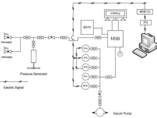
Figure 4.2 - Schematic diagram of the experimental apparatus used in the equilibrium measurements. ... 40
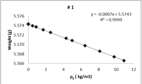
Figure 4.3 - Blank calibration of sample holder #1 used in the adsorption, using helium at 293.63K. ... 43
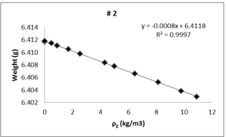
Figure 4.4- Blank calibration of sample holder #2 used in the adsorption, using helium at 293.63K. ... 44
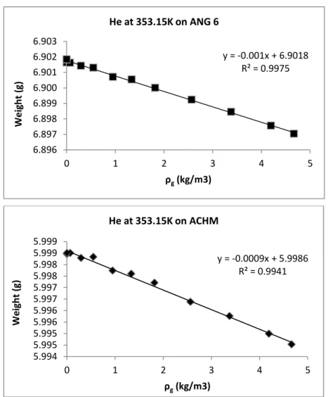
Figure 4.5 - Helium measurements on ANGUARD 6 (top) and ACHM (bottom) at 353.15K... 45
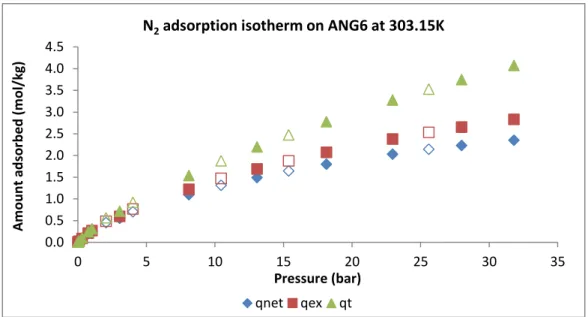
Figure 4.6 - Net (◊), excess (□) and total (∆) amount adsorbed for nitrogen (N2) at 303.15K for ANGUARD 6. The solid symbols represent adsorption and the open desorption. ... 47
Figure 4.7 - Sips model fitting of the N2 experimental data at 303K, 323K and 353K on ANGUARD 6 and parameters obtained. Symbols represent the experimental data and the surface is the global isotherm model. ... 49
Figure 4.8 - Single component N2 isotherms at 303K, 323K and 353K on the activated carbon ANGUARD 6.Symbols represent the experimental data (filled symbol – adsorption; empty symbol – desorption) and lines represent the fittings with the Sips model. The %ARE errors for 303.15K, 323.15K, and 353.15K are 6.98, 9.01 and 3.55, respectively. The N2 overall ARE error is 6.51%. ... 50
Figure 4.9 – Logarithmic representation of the single component N2 isotherms at 303K, 323K and 353K on the activated carbon ANGUARD 6.Symbols represent the experimental data (filled symbol – adsorption; empty symbol – desorption) and lines represent the fittings with the Sips model. The %ARE errors for 303.15K, 323.15K, and 353.15K are 6.98, 9.01 and 3.55, respectively. The N2 overall ARE error is 6.51%. ... 50
Figure 4.10 - Sips model fitting of the C4H10 experimental data at 303K, 323K and 353K on ANGUARD 6 and parameters obtained. Symbols represent the experimental data and the surface is the global isotherm model. ... 51
xvi
Sips model. The %ARE errors for 303.15K, 323.15K, and 353.15K are 3.90, 6.38 and 3.62, respectively. The C4H10 overall ARE error is 4.63%. ... 52 Figure 4.13- Sips model fitting of the CO2 experimental data at 303K, 323K and 353K onANGUARD 6 and parameters obtained. Symbols represent the experimental data and the surface is the global isotherm model. ... 52 Figure 4.14 - Single component CO2 isotherms at 303K, 323K and 353K on the activated carbon ANGUARD 6.Symbols represent the experimental data (filled symbol – adsorption; empty symbol – desorption) and lines represent the fittings with the Sips model. The %ARE errors for 303.15K, 323.15K, and 353.15K are 6.10, 6.20 and 8.45, respectively. The CO2 overall ARE error is 6.92%. ... 53 Figure 4.15 - Logarithmic representation of the single component CO2 isotherms at 303K, 323K and 353K on the activated carbon ANGUARD 6.Symbols represent the experimental data (filled symbol – adsorption; empty symbol – desorption) and lines represent the fittings with the Sips model. The %ARE errors for 303.15K, 323.15K, and 353.15K are 6.10, 6.20 and 8.45,
respectively. The CO2 overall ARE error is 6.92%. ... 53 Figure 4.16 - Sips model fitting of the CO2 experimental data at 303K, 323K and 353K on ACHM and parameters obtained. Symbols represent the experimental data and the surface is the global isotherm model. ... 54 Figure 4.17 - Single component CO2 isotherms at 303K, 323K and 353K on the activated carbon ACHM. Symbols represent the experimental data (filled symbol – adsorption; empty symbol – desorption) and lines represent the fittings with the Sips model. The %ARE errors for 303.15K, 323.15K, and 353.15K are 5.29, 4.33 and 6.49, respectively. The CO2 overall ARE error is 5.37%. ... 54 Figure 4.18 - Logarithmic representation of the single component CO2 isotherms at 303K, 323K and 353K on the activated carbon ACHM. Symbols represent the experimental data (filled symbol – adsorption; empty symbol – desorption) and lines represent the fittings with the Sips model. The %ARE errors for 303.15K, 323.15K, and 353.15K are 5.29, 4.33 and 6.49,
xvii
Figure 4.27 - Single-component adsorption isotherms of N2, C4H10 and CO2 on ANGUARD 6 at 303.15 K. The symbols represent the experimental data (filled symbol – adsorption; emptysymbol – desorption) and the lines represent the Sips model isotherm fitting. ... 60
Figure 4.28 - Selectivity of CO2/N2 as a function of pressure at 303.15K. ... 61
Figure 4.29 - Single-component adsorption isotherms for N2 (blue line), CO2 (green line), C4H10 (red line) on ANGUARD 6 and CO2 (purple line) on ACHM 6 at 303.15 K. ... 62
Figure 4.30 - Single-component adsorption isotherms for of CO2 on ANGUARD 6 and CO2 on ACHM 6 at 303.15 K. The amount adsorbed is represented in moles of carbon dioxide by mass of carbon sample. ... 63
Figure 4.31 - Single-component adsorption isotherms for of CO2 on ANGUARD 6 and CO2 on ACHM 6 at 303.15 K. The amount adsorbed is represented in moles of carbon dioxide by volume of carbon sample. ... 64
Figure A.1- BET Surface Area Report and BET Surface Area Plot for ANGUARD 6, obtained from DataMasterTM, V4.00 (2004). The value of is indicated as Qm. ... 80
Figure A.2 - t-Plot Report and t-Plot for ANGUARD 6, obtained from DataMasterTM, V4.00 (2004). ... 80
Figure A.3 - Horvath-Kawazoe Report for ANGUARD 6, obtained from DataMasterTM, V4.00 (2004). ... 81
Figure A.4 - Density Functional Theory results for ANGUARD 6, obtained from DataMasterTM, V4.00 (2004). ... 81
Figure A.5 - Intrusion Data from Hg porosimetry for ANGUARD 6 ... 81
Figure A.6 - Illustration of a piece of the ACHM used for the determination of its bulk density. . 83
Figure B.1 - Net (◊), excess (□) and total (∆) adsorption isotherms of nitrogen on ANGUARD 6 at 303.15K (top), 323.15K (middle) and 353.15K (bottom). ... 87
Figure B.2 -Net (◊), excess (□) and total (∆) adsorption isotherms of butane on ANGUARD 6 at 303.15K (top), 323.15K (middle) and 353.15K (bottom). ... 89
Figure B.3 - Net (◊), excess (□) and total (∆) adsorption isotherms of carbon dioxide on ANGUARD 6 at 303.15K (top), 323.15K (middle) and 353.15K (bottom). ... 91
Figure B.4 - Net (◊), excess (□) and total (∆) adsorption isotherms of carbon dioxide on the ACHM at 303.15K (top), 323.15K (middle) and 353.15K (bottom). ... 93
Figure C.1 - Magnetic Suspension Balance (Metal version). ... 99
Figure C.2 - Pressure Transducers from MKS Baratron and Omegadyne. ... 99
Figure C.3 - Unit controller for data acquisition by Rubotherm GmBH. ... 99
Figure C.4 - Gas Bottles from Air Liquid and Praxair. ... 99
Figure C.5 - Pressure Generator from HiP. ... 100
Figure C.6 - Thermostatic Bath, Refrigerator/Heater from Julabo. ... 100
Figure C.7 - Vaccum Pump from Edwards. ... 100
Figure C.8 - Heater from Nabertherm. ... 100
xix
List of Tables
Table 2.1 - Typical characteristics of activated carbons [36]. ... 16
Table 3.1 - PZC results obtained for ANGUARD 6. ... 19
Table 3.2 - PZC results obtained for the ACHM. ... 19
Table 3.3 - Values of nCFS for RUN A, RUN B, RUN C and RUN D. ... 23
Table 3.4 - (Continued) Values of nCFS for RUN A, RUN B, RUN C and RUN D. ... 24
Table 3.5 - Results obtained from t-plot method for ANGUARD 6. ... 29
Table 3.6 - Results obtained by HK method for ANGUARD 6. ... 30
Table 3.7 - Results obtained from Mercury Porosimetry for ANGUARD 6. ... 33
Table 4.1 - Blank calibration of the measuring cells... 44
Table 4.2 - Results obtained from helium measurements for ANGUARD 6 and ACHM. ... 45
Table 4.3 - Parameters obtained from Sips isotherm models for the pure gases in ANGUARD 6 and ACHM. ... 55
Table A.1 - Results from Bohem Titrations Experiments for RUN A – 48 hours without centrifugation (ANGUARD 6). ... 77
Table A.2 - Results from Bohem Titrations Experiments for RUN B – 48 hours with centrifugation (ANGUARD 6). ... 77
Table A.3 - Results from Bohem Titrations Experiments for RUN C– 24 hours with centrifugation (ANGUARD 6). ... 78
Table A.4 - Results from Bohem Titrations Experiments for RUN D – 48 hours with centrifugation (ACHM). ... 78
Table A.5 - N2 adsorption isotherm at 77K for ANGUARD 6. ... 79
Table A.6 - Characterization physical parameters of ANGUARD 6. ... 82
Table B.1 - Experimental data obtained from helium measurements at 353.15K for ANGUARD 6 and ACHM. ... 85
Table B.2 – Experimental nitrogen adsorption equilibrium data on the carbon sample ANGUARD 6 at 303.15K, 323.15K and 353.15K. 54 experimental data points were measured. ... 86
Table B.3 - Experimental butane adsorption equilibrium data on the carbon sample ANGUARD 6 at 303.15K, 323.15K and 353.15K. 40 experimental data points were measured. ... 88
Table B.4 - Experimental carbon dioxide adsorption equilibrium data on the carbon sample ANGUARD 6 at 303.15K, 323.15K and 353.15K. 43 experimental data points were measured. ... 90
Table B.5 - Experimental carbon dioxide adsorption equilibrium data on ACHM at 303.15K, 323.15K and 353.15K. 41 experimental data points were measured. ... 92
xxi
List of Symbols
Notation
- Dispersion constants for the adsorbate calculated from Kirkwood-Muller formulae (erg2.cm6) - Dispersion constants for the adsorbent calculated from Kirkwood-Muller formulae (erg2.cm6)
- Affinity constant (bar-1)
- Affinity constant at a reference temperature, (bar-1) – BET Constant
- Gas molecular diameter ( ̇) - Adsorbent atom diameter ( ̇)
- Average of the adsorbate and adsorbent molecule diameters ( ̇)
- Distance between the nuclei of two parallel infinite lattice planes or pore width ( ̇) - Weight read from the balance at any time (g)
- Mass of the sample holder (g) - Mass of the sample adsorbent (g)
- Kinetic energy of electron (0.8183x10⁻⁶ erg) – Sips isotherm model parameter
- Sips isotherm model parameter at the same reference temperature, - Amount adsorbed (cm3/g)
- Monolayer capacity (cm3/g)
- Number of moles of carbon surface functionalities at the carbon surface - Number of gas molecules per unit area (molecules/cm2)
- Avogadro’s number (6.023x10²³ molecules-1)
- Number adsorbent molecules per unit area (molecules/ cm2) – Absolute pressure (bar or mmHg)
- Saturated vapor pressure (bar or mmHg)
- Adsorbed quantity of the more adsorbed specie (mol/kg) - Quantity of the less adsorb quantity (mol/kg)
xxii
- Net adsorption (mol/kg)- Total amount adsorbed (mol/kg) - Maximum amount adsorbed (mol/kg)
– Heat of adsorption (kJ/mol)
or - Ideal gas constant (8.31441x10⁷ ergs/mole.K) – BET surface area (m2/g)
– Surface external area (m2/g) - Temperature (K)
- Standard multilayer thickness on the reference non-porous material at the corresponding relative pressure ( ̇)
Bulk volume (mL/g)
- Volume of all moving parts present in the measuring cell (cm3/g) – Microporous volume (cm3/g)
- Accessible pore volume of the adsorbent (cm3/g)
- Total porosity (%)
Skeletal volume in Hg porosimetry (mL/g)
- Specific adsorbent volume impenetrable to the adsorbate (cm3/g) - Diamagnetic susceptibility of an adsorbate atom (cm3)
- Diamagnetic susceptibility of gas molecule (cm3) - Isosteric heat of adsorption (kJ/mol)
Greek Letters
α - Sips isotherm model parameter - Polarizability of gas molecule (cm3) - Polarizability of adsorbent atoms (cm3) - Selectivity
- Cross-sectional area that each adsorbate molecule occupy in the completed monolayer (nm2)
- Density of the sample holder (g/cm3)
1
Chapter 1
1. Introduction
1.1. Motivation
Carbon dioxide (CO2) is naturally present in the atmosphere as part of the Earth's
carbon cycle (the natural circulation of carbon among the atmosphere and life beings). But since the Industrial Revolution, human activities have been altering the carbon cycle, by adding more CO2 to the atmosphere. It is now estimated that around 90% of the carbon dioxide present in
the atmosphere is from anthropogenic origin [1].
According to the Inventory of U.S Greenhouse Gas Emissions and Sinks (1990-2011) electricity production (38%), transportation of people and goods (31%) and industry (14%) are the sectors that most contribute to the emission of carbon dioxide to the atmosphere. This results from the burning of fossil fuels like coal, oil and natural gas [2]. Since carbon dioxide is a greenhouse gas, which can contribute to global climate change, it is imperial to reduce its emissions. In the past few decades many projects and possible solutions have been proposed to mitigate this problem. This includes improvements in energy efficiency and utilization of renewable and greener sources of energy [3].
Nowadays, CCS (CO2 Capture and Storage) is starting in several power plants [4]. CCS process consists in the capture of the carbon dioxide resulting from the burning of fossil fuels. CCS can be performed using pre-combustion or post-combustion techniques [5]. Then, after being separated from other gases, CO2 is compressed and transported through a net of pipelines or ships so it can be injected in underground geological formations, where it will be safely storage for several years. It is estimated that CCS process can reduce the emissions of carbon dioxide by 90% [6].
2
compressed. Despite being a mature process, amine scrubbing presents some drawbacks. Amine regeneration is very energy intensive, corrosion problems as well as the emission of carcinogenic compounds. Therefore, alternative processes are needed to overcome these difficulties [8].Adsorption-based separation processes are present important alternatives for CO2 capture from flue gases. Among this processes, Pressure Swing adsorption (PSA) is an important option. In this process the pressurized flue gas stream is passed through a porous solid that preferentially adsorbs CO2. After this, by decreasing the pressure, CO2 is desorbed and ready to be compressed [9].
The PSA performance and the power consumption of PSA is highly related with the adsorbents used. This is why the development of adsorbents with high adsorption capacities, high selectivity and good regenerability for CO2 adsorption/desorption is so important in the
design of the adsorption process. Many adsorbents have been studied for PSA application, including zeolites, activated carbons and, more recently metal organic frameworks. Among these materials activated carbons combine the advantages of being robust and also unexpansive materials [10].
1.2. Thesis Structure
This thesis is divided in five chapters:
Chapter 1: Introduction
The content of this chapter intends to advertise the reader about the problems related with the growing emissions of carbon dioxide to the atmosphere and how adsorption can be a viable alternative solution to help solve this problem.
This chapter also summarizes the organization of this work.
Chapter 2: Background
3
Chapter 3: Adsorbent CharacterizationThis chapter briefly explains the characterization methods used (Point of Zero Charge – PZC - method, Bohem titrations, N2 adsorption at 77K (BET Surface Area Method, t-Plot Method, Horvath-Kawazoe Method and Density Functional Theory Method) and Mercury Porosimetry and summarizes the results obtained for the activated carbons studied.
Chapter 4: Adsorption Equilibrium
In this chapter adsorption equilibrium data for carbon dioxide, nitrogen and butane on activated carbons are presented.
The apparatus and experimental procedure employed are described. Then, an explanation is given about the equations behind the several amounts adsorbed considered. The concepts of absolute, excess and net amount adsorbed are discussed and the corresponding results obtained are presented. The experimental data obtained was fitted with the Sips isotherm model and the obtained results are presented and discussed.
Chapter 5: Conclusions and Suggestions for Future Work
5
Chapter 2
2.
Background
2.1. Adsorption
2.1.1. Definition
Adsorption can be defined as the process where some atoms, ions or molecules present in a given fluid, gas or a liquid (adsorptive), adhere to the surface of a solid material (adsorbent). Due the increase of the adsorptive compound concentration, the solid material will be enriched with the molecules of the fluid phase. This molecules adsorbed on the surface of the solid material can be referred as adsorbate.
The reverse process, called desorption, can be defined as the removal of adsorbate from the adsorbent. Desorption can be promoted by the decreasing the pressure and/or increasing the system temperature [11].
2.1.2. Some Applications
Adsorption phenomena is related with important technology processes used nowadays, not only because some adsorbents are used in large scale as desiccants, catalysts or catalyst supports but also because adsorption can be used in areas so diverse like separation of gases, purification of liquids and pollution control, like the removal of aqueous contaminants from groundwater [12]. This phenomenon is also useful for the determination of the surface area and pore size distribution of a diverse range of powders and porous materials [13].
2.1.3. Chemisorption and Physisorption
6
a) Since in chemisorption the molecules of the fluid phase react with the adsorbent
molecules, its original form is not kept. On the other hand, in physisorption, the molecules are adsorbed and desorbed without any chemical reaction.
b) Physisorption has a relatively low degree of specificity and for that adsorbate molecules can be linked to other adsorbate molecules and to the adsorbent, forming multilayers. On the other hand, chemisorption is dependent on the reactivity of the adsorbent and adsorptive, so adsorbate molecules can only linked to specific sites of the adsorbent surface, being confined to a monolayer.
c) The energy of chemisorption has the same order of magnitude as the energy change in a comparable chemical reaction. Physisorption is always exothermic, but the energy involved is, generally, not much higher than the energy of condensation of the adsorptive.
2.1.4. Adsorption Isotherms
The relation, at constant temperature, between the amount adsorbed and the equilibrium pressure (for gases) is known by adsorption isotherm. When the adsorptive pressure stabilizes, the equilibrium is reached, which means that the quantity of molecules adsorbed and the molecules in the fluid phase will not vary with time
In order to describe this relation there are several models of isotherms. However the isotherm models of Freudlich, Langmuir and BET (Brunauer, Emmett and Teller) are the most commonly observed [14]. A typical gas adsorption isotherm is represented by a plot of the amount adsorbed versus the adsorptive pressure. The pressure can also be expressed as a ratio of the adsorptive pressure, P, to the saturated vapor pressure, .
7
Figure 2.1 - IUPAC gas physisorption isotherm classification [13].The different adsorption isotherm types are related with the adsorbent and adsorbate properties. The differences between them can be listed as follow.
Type I - Observed in the physical adsorption of gases on microporous solids, in which
the pore size is not much greater that the molecular diameter of the adsorbate molecule. This type of adsorption isotherm is common in activated carbons and black carbons [15].
Type II – Typically observed in non-porous or macroporous adsorbents. An inflexion
point, or knee, is indicated by point B in Figure 2.1. This point indicates the stage at which the monolayer coverage is complete and multilayer adsorption begins to occur [16].
Type III – Observed in macroporous solids. This isotherm is convex to the ( / ) axis
over its entire range and therefore does not exhibit a point B. This feature is indicative of weak adsorbent/adsorbate interactions. These kinds of isotherms are not common [13], [16].
Type IV – Characteristic of mesoporous adsorbents, this kind of adsorption isotherm
possess a hysteresis loop (which means that the adsorption isotherm is different from the desorption isotherm).Type IV isotherms are common but the exact shape of the hysteresis loop varies with the system properties [13], [15].
Type V – Like the previous type, this isotherm is observed mesoporous solids and
8
Type VI – Usually observed on porous solids with uniform surfaces, this kind of
isotherm is relatively rare and is associated with layer-by-layer adsorption on a highly uniform surface [13].
This type of isotherm classification is only applicable to the adsorption of a single-component gas within its condensable range of temperature. Such measurements are extremely useful for the characterization of porous materials [13].
2.1.5. Measuring Adsorption Isotherms
In order to determine the adsorption isotherms and the energies associated with the adsorption phenomena, experimental measurements must be made. Depending on the gas-solid system in study and the operational conditions there are several gas adsorption methods to quantify the amount adsorbed. The most used are the volumetric and gravimetric methods.
2.1.5.1.
The Volumetric Method
The name volumetric method dates from the Emmett and Brunauer (1937) [13] experiments which were made using a mercury burette and a manometer. This technique is based on the measurement of the gas pressure in a calibrated constant volume at a known temperature.
A typical volumetric apparatus, shown in Figure 2.2, possess two different chambers: one for the adsorbent sample is placed and other for the calibrated charge volume. Initially, the adsorbent contained in the adsorption cell (or chamber) is activated under the appropriate conditions in order to remove the previously adsorbed species. Both the column and the reservoir are maintained at the desired temperature. After this, the reservoir is charged with the gas to a predetermined pressure. The valve between the reservoir and the column is then opened, and the adsorption equilibrium is established between the solid and the gas; the final equilibrium pressure is recorded [17].
9
Figure 2.2 - Generic volumetric apparatus [17].2.1.5.2.
The Gravimetric Method
The determination of the amount adsorbed by the gravimetric method using a spring balance was first use by McBain and Bakr in 1926. The apparatus consisted in an adsorbent bucket attached to the lower end of a fused silica spring, which was suspended within a vertical glass tube. Nowadays, spring balances have been substituted by suspension magnetic balances (MSB) [13].
The process is initiated by placing the adsorbent sample inside a basket. The material is then activated preferentially in-situ, in vacuum at a desired temperature. After the sample is cleaned from impurities, the first measurement will give weight of the pair basket + clean adsorbent sample. After this, adsorbate is fed to the adsorption chamber and the sample is then allowed to equilibrate at the desired pressure and temperature (at a gas molar density). The signal from the microbalance is recorded under equilibrium conditions (pressure and temperature are constant). The change in the microbalance signal is a result of adsorption occurring on the solid surface and the total buoyancy force [17]. A generic gravimetric apparatus is shown in Figure 2.3.
10
Figure 2.3 - Generic gravimetric apparatus [17].2.2. Adsorbates
The following gases were selected for the present work since they are adsorbates with interest in typical adsorption applications. Moreover, those gases are of extreme importance in the mitigation of the greenhouse gas emissions.
2.2.1. Carbon Dioxide
Carbon dioxide, CAS number [124-38-9], CO2, Mr 44.010 g/mol, with a boiling point of -329.72K (56.57ºC) and a melting point of 193.33K (-78.92ºC) is a colorless, odorless, non-flammable gas with a sour taste. At normal temperature, the carbon dioxide molecules are relatively stable and do not readily break down into simpler compounds. However, the substance is very sensitive to high temperatures, ultraviolet light, and electrical discharge [18].
11
2.2.2. Nitrogen
When two molecules of elemental nitrogen, N (atomic number 7, Ar 14.0067 g/mol) form a stable diatomic molecule they origin a molecular substance named nitrogen, CAS number [7727-37-9], N2, Mr 28.0134 g/mol. At atmospheric pressure and room temperature, nitrogen is a colorless, odorless, noncombustible gas. Nitrogen has a boiling point of 77K (at 1.01 bar) and a melting point of 63.29K (−209.86 ºC).
Nitrogen, which means “lifeless” in Greek, was named by Lavoisier. This molecule is obtained from air and is one of its major constituents (78%). In industry, cryogenic (low-temperature) processes, adsorption processes (such as PSA – Pressure Swing Adsorption), and membrane separation are used to separate nitrogen from air [18]. Also, N2 is one of the main components of flue gases and, therefore, the knowledge of its adsorption properties is extremely important for the modelling of adsorption-based processes for CO2 capture from flue gases [1].
2.2.3. Butane
Butane, CAS number [106-97-8], C4H10, Mr 58.122 g/mol, with a boiling point of 273.65K (0.5ºC) is a gaseous hydrocarbon with a colorless and odorless aspect. This substance currently known as n-butane (to indicate that the carbon atoms are linked in a straight chain) occurs in natural gas and in crude oil. It is formed in large quantities, by catalytic cracking in the refining of petroleum to produce gasoline. Commercially, n-butane can be added to gasoline to increase its volatility [21]. Removal of butane from natural gas and biogas is extremely important, reason why the study of its adsorption equilibrium is of major importance for the design of adsorption based processes [22].
2.3. Adsorbents
2.3.1. General Adsorbents
Adsorbents are porous solid materials which have the ability to adsorb molecules from a liquid or gas [14]. According to IUPAC [23], the pore size generally specified as pore width (the available distance between two opposite walls) of a porous material can be classified as:
Micropore– Pore of internal width less than 2 nm;
Mesopore - Pore of internal width between 2 and 50 nm;
12
The potential of adsorbents has been studied since the 18th century [14] and the applications for the use of adsorbents have grown with the years. For this reason, it became necessary to design new adsorbents in order to face the specificity of the processes, which they are applied. Some of the most important application for adsorbents are:a) Gas separation processes like the upgrading of biogas [24];
b) Cleaning processes, sewage gas purification [25], removal of contaminants from groundwater through adsorption [12] and the cleaning of industrial effluents [26];
c) Gas storage processes like Adsorbed Natural Gas (ANG) [22];
According to the gas adsorption process, a proper selection of the adsorbent must be made. Nowadays there are several adsorbents available. Some of them are listed next.
The name activated alumina is generally applied to an alumina adsorbent prepared by the heat treatment of some hydrated alumina (i.e. a crystalline hydroxide, oxide-hydroxide or hydrous alumina gel) [13]. This material presents a good mechanical resistance and can be used in moving bed applications [27]. The surface chemistry of activated alumina, as well as its pore structure, can be modified by the use of a controlled thermal treatment [28].
Silica Gel has a granular and amorphous form. It is produced by heating a gel, product
of the acidification of a solution of sodium silicate. This glassy material is highly porous and it is used to dry liquids and gases and also to recover hydrocarbons [27]. In addition, its surface can be modified by reacting (or grafting) with a monomolecular layer of organic ligand. These modified silica gels can be applied in several chromatographic applications [28].
Zeolites, also referred to asmolecular sieves, are microporous crystalline solids with
well-defined structures. Generally they contain silicon, aluminum and oxygen in their framework and cations, water and/or other molecules within their pores. Many zeolites occur naturally as minerals as others are synthetic. The major use of zeolites are in petrochemical cracking, ion-exchange (water softening and purification), and in the separation and removal of gases and solvents [29].
Metal-Organic Frameworks (MOFs) are crystalline materials composed of two
13
Once the adsorbents used in this work are two activated carbons, a special section will be dedicated to these materials.2.3.2. Activated Carbon
2.3.2.1. Historical Aspects
The first known use for carbon dates from Egyptian time, where this material was used for oil purification and medicinal purposes. By the early 19th century both wood and bone charcoal were used in large-scale for the decolorization and purification of cane sugar [27], [28], [34].
However, it was only in the beginning of the First World War (WWI) that the potential of activated carbon was really capitalized upon. The advent of gas warfare necessitated the development of suitable respiratory devices for personnel protection. Granular activated carbon was used to this end as, indeed, it still is today [35]. By the late 1930’s there was considerable industrial-scale use of carbon for gaseous and liquid phase application. During the Second World War (WWII), a more sophisticated chemically impregnated carbon for entrapment of nerve gases was produced [34].
2.3.2.2. Structure and Precursor Materials
14
Figure 2.4 - Hexagonal structure of graphite [13].Depending on the raw materials used for its production, several types of activated carbon can be obtained. Almost all materials containing high fixed carbon content can potentially be activated. The most used carbonaceous source materials are coal (anthracite, bituminous, sub-bituminous and lignite), coconut shell, peanut shell, wood, peat, coals, petroleum coke, bones and fruit nuts. Among these, anthracite and bituminous coals have been the major sources employed [27], [28], [38], [39].
2.3.2.3. Carbonization and Activation
The process for the production of activated carbon usually involves three steps: a) Raw material preparation, b) Carbonization and c) Activation. In order to achieve the desired pore structure and mechanical strength, the activation conditions must be carefully controlled. There are two kinds of activation: physical activation and chemical activation. In both a step of carbonization is required. This step allows the pure carbon to be extracted by pyrolysis [12], [40].
In physical activation, once the material is carbonized it is exposed to oxidizing gases
like carbon dioxide, oxygenor steam, under a temperature usually between 1073.15K and 1273.15K. This activation step serves to create porosity allowing the tailoring of the desired size distribution and surface area.
In chemical activation the materialis first impregnated with chemicals agents such as
phosphoric acid or zinc chloride and then is carbonized [12], [28], [41].
15
Figure 2.5 - Schematic representation of an activated carbon porous matrix [42].2.3.2.4. Applications
Due to its unique adsorptive characteristics, activated carbon plays an important role in many liquid and gas phase applications [43]. Some of the processes that use this adsorbent are listed as following:
Because of its large surface area, purity and relative hardness, activated carbon is an ideal carrier for catalytic metals, for example in batteries [44]. In the environmental field, adsorption over activated carbon it is used for several applications. Some of these applications are effluent treatment of industrial and municipal waste waters, air purification and capture of volatile organic compounds (VOC’s) from diverse streams, and the removal of pesticides from contaminated soils [12], [44]. In medicine, activated carbons can be employed in poisoning treatments.Through its ingestion, this material prevents the poison from being absorbed in the stomach. Sometimes, several doses of activated charcoal are needed to treat severe poisoning [45].
Activated carbons present a great option for gas storage, especially for natural gas. Because they have a large microporous volume, are efficiently compacted into a packed bed, and can be cheaply manufactured in large quantities [22], [46]. This procedure permits storing the gas at lower pressures, improving the safety criteria and reducing the compression costs associated to the traditional storage methods [22].
Cane and sugar syrups require decolorization before being ready for final use. Activated carbons are specially processed to develop pore structures that readily adsorb plant pigments from the sugar (polyphenols) [47].
16
available at low, prices, and being present in industry for so long, they are considered a robust material for adsorption applications. In Table 2.1 it is possible to see some typical characteristics of activated carbons.Table 2.1 - Typical characteristics of activated carbons [36].
True density 2.2 g/cm3 Particle density 0.73 g/cm3 Total porosity 0.71 Macropore porosity 0.31 Micropore porosity 0.40 Macropore volume 0.47 cm3/g Micropore volume 0.44 cm3/g Specific surface area 1200 m2/g Mean macropore radius 800 nm Mean micropore half width 1-2 nm
17
Chapter 3
3. Adsorbent Characterization
3.1. Introduction
The design of a separation or purification process by adsorption begins with the choice of a suitable adsorbent. The success or failure of the process is strictly related with the performance of the adsorbent in both adsorption equilibria and kinetics. To satisfy these two requirements the adsorbent must have [36]:
a) A reasonable high surface and a micropore volume, so it can have a good adsorption capacity;
b) Relatively large pore network: If the pore size is too small the transport of the gas molecules to the particle interior can take too long influencing the kinetics;
c) An easy desorption: If the adsorbent does not have properties that allow an easy desorption, it will be necessary to expose the material to high temperatures or extremely low pressure for its regeneration. This will contribute to reduce the adsorbent life due to thermal ageing [15] and increases the energy consumption related to adsorbent regeneration.
Therefore, in order to evaluate the adsorbent, adsorbent characterization must be performed. Density, surface area, pore size distribution, pore volume, and the surface chemistry are usually determined. In this study, an activated carbon, ANGUARD 6 (ANG 6), in the form of extrudates with 1mm diameter, supplied by Sutcliffe Speakman Carbons Ltd. (UK) was characterized at FCT/UNL using N2 adsorption at 77K, Mercury porosimetry, Bohem Titration Method, Point of Zero Charge Method (PZC) and Thermogravimetric Analysis (TGA).
During the realization of this work, another carbonaceous material became available and, therefore, was possible to perform the PZC and Bohem titrations analysis for this sample. This material consists in an activated carbon honeycomb monolith (ACHM) purchased from Master Carbon International Limited (UK). The monolith is cylindrical and presents 20 mm of external diameter and 300 cells per square inch. Erro! Auto-referência de marcador inválida. shows the two carbon samples.
18
3.2. Characterization Methods
3.2.1. Point of Zero Charge (PZC)
3.2.1.1 General Description
The surface of a carbon particle is basic or acidic depending on the functional groups that are in majority on its surface. When a small amount of well crushed activated carbon is mixed with water, the ions H+ and OH- from the dissociation of the functional groups are given to the solution until the acid/base equilibrium is achieved. PZC (Point of Zero Charge) is a widely used method to determine the surface nature of a carbonaceous adsorbent and can be defined as the pH value at which a solid submerged in an electrolyte exhibits zero net electrical charge [12], [48].
3.2.1.2. Experimental Procedure
Conditions:
An aqueous solution with 0.5 g of well crushed ANGUARD 6 and 50 mL of distillated water was prepared. The glass container in which the solution was kept covered with an aluminum sheet to prevent the oxidation of the carbon. After that, the solution was subject to agitation during 48 hours, at 200 rpm. Thereafter, the agitation was stopped and the solution allowed standing. Then, using a graduated pipette an aliquot was collected from the solution and its pH value was determined using a digital pHmeter, CRISON 2001.
To secure the data reproducibility, three PZC experiments were made. In the first two, the carbon was allowed to settle in the bottom of the vessel and the aliquots were collected from the solution above the settled carbon. However, for the third experiment the solution was subject to centrifugation and the supernatant removed. This procedure enhanced the time needed to read pH in the digital pHmeter employed, since there were less carbon particles in suspension.
PZC analysis was also performed for the activated carbon monolith. Since the amount of material available for the experiments was less than for ANGUARD 6, the experimental protocol had to be modified. This way, half the quantity of activated carbon and distilled water were employed. Also, after the agitation step the carbon solutions were centrifuged.
19
3.2.1.3. Experimental Results and Data Analysis
The results obtained from PZC experiments for ANGUARD 6 and the ACHM are presented in Table 3.1 and Table 3.2 respectively.
Table 3.1 - PZC results obtained for ANGUARD 6.
Experiment Weight of ANG 6 (g) pH value
1* 0.513 7.08 at 293.55K
2* 0.512 7.06 at 292.35K
3** 0.513 6.81 at 293.15K
*without centrifugation, ** with centrifugation, pH of distillated water: 5.35 at 293.55K.
Table 3.2 - PZC results obtained for the ACHM.
Experiment Weight of ANG 6 (g) pH value
1* 0.256 6.15 at 293.15K
2* 0.254 6.67 at 293.15K
3* 0.257 6.50 at 293.15K
* with centrifugation, pH of distillated water: 4.89 at 293.15K.
From the results obtained, the average pH value obtained for ANGUARD 6 was 6.98 and for the ACHM the average pH was 6.44. It can be concluded that the surface of both activated carbons is amphoteric, which means that the acid and basic surface functional groups are in equilibrium.
3.2.2. Bohem Titration Method
3.2.2.1 General Description
Many properties of carbon materials, in particular their adsorption behavior are influenced by the chemisorbed oxygen. The oxygen present on the surface of an activated carbon can bond with several elements such as oxygen, nitrogen, hydrogen and sulphur to form functional groups. According to the activation method used, the functional groups present in the surface of a carbon can be different. Acidic and basic surface sites usually coexist, but the concentration of basic sites decreases with the increasing acid character of the surface and vice-versa. The functional groups usually found in activated carbons are: carboxyl, carboxylic anhydride, lactone, lactol, phenol, carbonyl (acidic groups) and chromene, ketone and pyrones (basic groups) [15], [48] . Some of these functional groups can be seen in Figure 3.2 and
20
Figure 3.2 - Simplified schematic of some acidic surface groups on an activated carbon [28].Figure 3.3 - Schematic of some possible basic groups on an activated carbon [28].
The Boehm titration method permits the identification of the functional groups present in the carbon surface. For this purpose, a small amount of activated carbon is mixed with some strong bases in order to neutralize the phenols, lactonic groups and carboxylic acids. These basic substances are NaOH, Na2CO3 and NaHCO3. Sodium hydroxide (NaOH) is the strongest base and neutralizes all the Brönsted acids, while sodium carbonate (Na2CO3) neutralizes carboxylic acids and lactonic groups (e.g. lactone) and sodium bicarbonate (NaHCO3) neutralizes carboxylic acids. The number of basic sites is calculated from the amount of HCl required to the titration [48].
3.2.2.2. Experimental Procedure
For determination of the acidic and basic surface functional groups of ANGUARD 6 three laboratorial experiments were performed. The experimental procedure was initiated by the preparation of the basic and acidic solutions.
Solutions preparation:
21
RUN A Procedure:From each solution, 10 mL were extracted to glass containers and 1.0 g of well crushed ANGUARD 6 was added. The glass containers were covered with an aluminum sheet to prevent the oxidation of the carbon particles through the exposure to humid air. The solutions were subjected to a period of agitation of 48 hours, at 200 rpm.
After this period, the agitation was stopped and the solutions were left to settle, during 10 to 15 minutes. In order to remove most of the carbon particles the solutions were decanted several times. Then, aliquots were extracted with a graduated pipette and their pH values were measured. Finally, the basic and acidic titrations were made, using as titrants an aqueous solution of NaOH (0.1 M) and an aqueous solution of HCl (0.1 M). Two drops of phenolphthalein were used as pH indicator.
RUN B Procedure:
The conditions and procedure used in this experiment were the same as the ones used
for RUN A, with the difference that after the agitation, the solutions were centrifuged to obtain a
better separation between the two phases (liquid and solid).
RUN C Procedure:
From each solution, 10 mL were extracted and 1.0 g of non-crushed ANGUARD 6 was added. The glass containers were covered with aluminum sheet to prevent the oxidation of the carbon particles through the exposure to air humidity. The solutions were subjected to a period of agitation of 24 hours, at 200 rpm.
Thereafter, the agitation was stopped and the solutions were subject to centrifugation. The aliquot was then extracted and the pH values were measured. Finally, the basic and acidic titrations were made, using as titrants aqueous solutions of NaOH (0.1 M) and HCl (0.1 M). Again, phenolphthalein was employed as pH indicator.
The calculations used for this analysis can be consulted in APPENDIX A.1.
3.2.2.3. Experimental Results and Data Analysis
22
inefficient because not only the waiting for the carbon mixture to settle adds substantial time to the experiment but also the carbon particles left in the supernatant add difficulty the pH lecture.The mass, volume and concentrations values obtained for the four experimental procedures can be seen in APPENDIX A.2, Table A.1 to Table A.3 (for ANGUARD 6) and in
Table A.4 (for the ACHM).The values of for each functional group per gram of adsorbent
are presented in Table 3.3 and Table 3.4.
After the analysis of the results obtained for the four experiments, it was observed that the values of for the lactones were always negative. Since there is no such thing as negative number of moles, the values were considered to be zero. This means that the surface of both activated carbons is not characterized by lactonic groups.
23
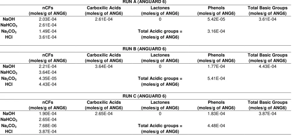
Table 3.3 - Values of nCFS for RUN A, RUN B, RUN C and RUN D.
RUN A (ANGUARD 6)
nCFs Carboxilic Acids Lactones Phenols Total Basic Groups
(moles/g of ANG6) (moles/g of ANG6) (moles/g of ANG6) (moles/g of ANG6) (moles/g of ANG6)
NaOH 2.03E-04 2.61E-04 0 5.42E-05 3.61E-04
NaHCO3 2.61E-04
Na2CO3 1.49E-04 Total Acidic groups = 3.16E-04
HCl 3.61E-04 (moles/g of ANG6)
RUN B (ANGUARD 6)
nCFs Carboxilic Acids Lactones Phenols Total Basic Groups
(moles/g of ANG6) (moles/g of ANG6) (moles/g of ANG6) (moles/g of ANG6) (moles/g of ANG6)
NaOH 2.21E-04 3.64E-04 0 1.77E-04 4.43E-04
NaHCO3 3.64E-04
Na2CO3 4.35E-05 Total Acidic groups = 5.41E-04
HCl 4.43E-04 (moles/g of ANG6)
RUN C (ANGUARD 6)
nCFs Carboxilic Acids Lactones Phenols Total Basic Groups
(moles/g of ANG6) (moles/g of ANG6) (moles/g of ANG6) (moles/g of ANG6) (moles/g of ANG6)
NaOH 1.90E-04 2.65E-04 0 1.83E-04 3.87E-04
NaHCO3 2.65E-04
Na2CO3 7.68E-06 Total Acidic groups = 4.48E-04
HCl 3.87E-04 (moles/g of ANG6)
24
Table 3.4 - (Continued) Values of nCFS for RUN A, RUN B, RUN C and RUN D.RUN D (ACHM)
nCFs Carboxilic Acids Lactones Phenols Total Basic Groups
(moles/g of ACHM) (moles/g of ACHM) (moles/g of ACHM) (moles/g of ACHM) (moles/g of ACHM)
NaOH 1.17E-04 1.32E-04 0 8.45E-05 3.04E-04
NaHCO3 1.32E-04
Na2CO3 3.30E-05 Total Acidic groups = 2.17E-04
HCl 3.04E-04 (moles/g of ACHM)
25
3.2.3. Thermogravimetric Analysis (TGA)
3.2.3.1 General Description
Thermogravimetric analysis (TGA) is a procedure that allows the evaluation of the physical and chemical properties of materials with the increase in temperature. Usually, the weight of the analyzed sample is measured while the temperature is increased. The results are generally plotted in a curve of the weight percentage versus temperature. Through this analysis is possible to know the percentage of the impurities or volatile components, including humidity, lost in the degassing process of an adsorbent. It is also possible to know which is the maximum temperature to which an adsorbent can be subjected without contributing for its decomposition [49]. This analysis can be performed in equipments that combine extremely precise balance and a programmable furnace for temperature control.
3.2.3.2. Experimental Results and Data Analysis
A sample of ANGUARD 6 (8.4720 mg) was analyzed by TGA (TGA model Q50 V6.7 Build 203, Universal V4.4A TA Instruments - USA) to determine the temperature interval over which the sample decomposes. This was done by recording the weight loss as a function of increasing temperature. The analysis was performed under a nitrogen atmosphere at a heating rate of 278.15K/min (5ºC/min).
The TGA profile obtained is showed Figure 3.4:
Figure 3.4 – TGA analysis of ANGUARD 6.
26
873.15K (600ºC) the sample starts to decompose so it is clearly not advisable to heat the adsorbent sample in the activation process more than 823.15K (550ºC). Employing adsorbent activation temperatures between 323.15K and 473.15K (50ºC and 200ºC) the weight decrease is around 3 to 4%.3.2.4. Nitrogen adsorption at 77K
3.2.4.1 General Description
Nitrogen adsorption at 77K was performed for the activated carbon ANGUARD 6. The experiment was performed using a static volumetric apparatus (ASAP 2010, Micromeritics Adsorption Analyzer, USA) in a range of relative pressure 10-6<P/P
0<0.99. The sample weight used in the experiment was 0.1418 g. The data from the isotherm was then analyzed using the software DataMasterTM, V4.00 (2004). The data obtained from the isotherm of N2 at 77K measured are presented in APPENDIX A.3, Table A.5. Figure 3.5 shows the isotherm obtained.
Figure 3.5 - Adsorption isotherm of N2 at 77K for ANGUARD 6.
3.2.4.1.1. BET Surface Area Method
Brunauer, Emmett and Teller (BET) method is commonly used to determine the surface area of porous materials. Brunauer, Emmett and Teller (1938) extended the Langmuir mechanism to multilayer adsorption and obtained an isotherm equation (BET equation). It is assumed that the adsorbate molecules can settle on the adsorbent surface or on the top of another adsorbate molecule [13].
0 100 200 300 400 500 600 700 800
0.0 0.2 0.4 0.6 0.8 1.0 1.2
27
The first step is to determine the monolayer capacity, through the BET Equation [13], [50]:
(Equation 3.1)
Where, is the amount adsorbed in cm3/g, is the absolute pressure in mmHg, is the saturation pressure in mmHg and is the BET constant.
By simplifying Equation 3.1, a linear relation can be established between
and .
(Equation 3.2)
This relation can be plotted, where the slope is s =
and the intercept is a = .
By solving these two equations simultaneously, it can be obtained:
(Equation 3.3)
(Equation 3.4)
To guarantee the linear region of a BET plot it is recommended to restrict the values of relative pressure to a range of 0.05-0.3 . However, the advisable procedure is to obtain, by a statistical analysis, the best linear fit for the initial part of the isotherm [13].
Then, next step is to calculate the BET surface area, , the surface area that will be available for adsorption, using that was obtained from Equation 3.3:
(Equation 3.5)
28
By restricting the relative pressure range between 0.025 to 0.31 , DataMasterTM generated a BET Surface Area Report and a BET Surface Area Plot, shown in APPENDIX A.4,Figure A.1.
The recommended procedure is to obtain the best linear fit for initial part of the isotherm. Using only the experimental points in the BET relative pressure range, the fitting obtained was not so good. By extending the relative pressure range, using the previous point ( = 0.025), the correlation coefficient obtained was higher (0.9976), indicating a better fitting.
According to the BET theory, the BET constant is related exponentially to the enthalpy (heat) of adsorption in the first adsorbed layer [51]. Because of this, the value must be positive. If the value is negative this means that the relative pressure range chosen is not adequate [13]. Since the value for obtained for this analysis was =106.50 (>0), the choice of the relative pressure range was assumed to be adequate. Also, since the BET theory is an extension of the Langmuir mechanism to multilayer adsorption, to consider the value reliable, it is necessary that the knee of the isotherm is fairly sharp (i.e. the BET constant is not less than ~100) (12).The BET surface area obtained for ANGUARD 6 is 1699.79 m²/g which is within the typical range for activated carbons (between 300 and ∼ 4000 m2/g) [28].
3.2.4.1.2. t-plot Method
The t-plot method was proposed by Lippens and Boer in 1965. This method allows the determination of micropore volume, external surface and micropore area. The experimental from the isotherm is redrawn in a t-curve, i.e., a plot of the quantity of gas adsorbed as a function of t, the standard multilayer thickness on the reference non-porous material at the corresponding . These t-values are calculated using a thickness equation (Equation 3.6). When the shape of the reference t-curve and experimental isotherm do not coincide, that is an indication that a non-linear region was reached. From the point where the non-linear region begins, a line is drawn (extrapolated) to intercept the yy axe (t=0). The values of external surface area and micropore volume can be determined from the intercept and slope obtained [13].
DataMasterTM V4.00 uses Harkins and Jura Equation (1944) to determine the values of thickness [52].
( ̇) √ ( )
29
Through the slope, s, of the extrapolation is possible to calculate the external surface area in m2/g and from the intercept, a, the micropore volume in cm3/g [16].(Equation 3.7)
(Equation 3.8)
The micropore area, in m2/g can be calculated through the difference between the BET surface area and the external surface area.
(Equation 3.9)
According to the literature [16] the t-plot method is valid for a relative pressure range of 0.08 to 0.75 . The results obtained for ANGUARD 6 can be seen in APPENDIX A.5,
Figure A.2. By restricting the relative pressures to the range recommended, the obtained
correlation coefficent was close to 1, which indicates a good fitting. According to the results found in the literature [13], the values obtained are in acordance with the values for several activated carbons. Table 3.5 presents a resume of micropore volume, external surface area and micropore surface area for the activated carbon ANGUARD 6:
Table 3.5 - Results obtained from t-plot method for ANGUARD 6.
Micropore Volume
(cm3/g)
External surface area
(m2/g)
Micropore surface area
(m2/g)
0.94 52.50 1647.29
3.2.4.1.3. Horvath-Kawazoe (HK) Method
Horvath and Kawazoe (HK) described a semi-empirical, analytical method for the determination of effective pore size distributions from N2 adsorption isotherms in microporous materials. In its original form, the HK analysis was applied to nitrogen isotherms determined on molecular sieve carbons, over the assumption that these adsorbents contained slit-shaped graphitic pores. However, nowadays it can be applied to other adsorbents with different pore geometries like zeolites [13], [16].
30
( ) (Equation 3.10)Much of the physical parameters present in this equation can be easily found in the literature [28], [53], [54]. The nomenclature for equations Equation 3.10 to Equation 3.14 can be found in List of Symbols (Page XXI to Page XXIII). Others like the dispersion constants and the inter-nuclear distances must be calculated employing [16], [55]:
(Equation 3.11)
(Equation 3.12)
( )
(Equation 3.13)
( )
(Equation 3.14)
DataMasterTM analysis allowed obtaining the results presented in Table 3.6:
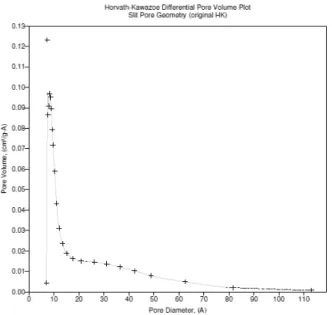
Table 3.6 - Results obtained by HK method for ANGUARD 6.
Maximum Pore Volume
(cm3/g)
Medium Pore Diameter
̇
0.98 18.4
The Horvath-Kawazoe detailed report for ANGUARD 6 is present in APPENDIX A.6.,
31
Figure 3.6 - Micropore size distribution obtained from Horvath-Kawazoe Method for ANGUARD 6.The pore size distribution results obtained from HK Method for ANGUARD 6 shows that most of the pores lie in the micropore region (<20 ̇), but also reveals the existence of small mesopores for pore widths slighty higher than 20 ̇.
3.2.4.1.4. Density Functional Theory (DFT) Method
Density functional theory (DFT) is a quantum mechanical modelling method mostly used in physics and chemistry areas. In chemistry, it has a great use for predicting a great variety of molecular properties like molecular structures, vibration frequencies, atomization energies, ionization energies, electric and magnetic properties, reactions paths, etc. [56] .
In adsorption science, this statistical method attempts to extend the accuracy of pore size distribution analysis in both micropore and mesopore range [15]. DFT and Gibbs Ensemble Monte Carlo molecular simulation (GEMC) represent an alternative to the classical methods, like the HK method. Usually, for activated carbon it is assumed that the material is composed of non-interconnected, slit-shapes pores with chemically homogeneous graphitic surfaces.
32
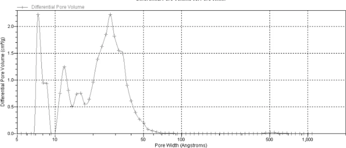
Figure 3.7 - Pore size distribution obtained from DFT Method for ANGUARD 6.As it was seen for the HK Method, the DFT analysis confirms that the sample adsorbent is mostly microporous, but the existence of mesopores with pore widths slightly above 20 ̇ is confirmed.
3.2.5. Mercury Porosimetry
3.2.7.1 General Description
Mercury porosimetry characterizes the porosity of a given material by applying various levels of pressure to a sample immersed in mercury. The pressure required to intrude mercury into the sample pores is inversely proportional to the size of the pores. This indicates that at first, macropores and mesopores are filled with mercury and just then, the mercury enters in the micropores. In spite of the pressure applied, this method is reserved to the analysis of the characteristics of larger pores, instead of the smaller pores [57].
![Figure 2.1 - IUPAC gas physisorption isotherm classification [13].](https://thumb-eu.123doks.com/thumbv2/123dok_br/16481252.732424/31.892.237.653.112.411/figure-iupac-gas-physisorption-isotherm-classification.webp)
![Figure 4.1 - Magnetic suspension balance components [60].](https://thumb-eu.123doks.com/thumbv2/123dok_br/16481252.732424/62.892.133.762.106.880/figure-magnetic-suspension-balance-components.webp)