www.scielo.br/rbg
IMPACTS OF SEISMIC VELOCITY MODEL CALIBRATION FOR TIME-DEPTH CONVERSION:
A CASE STUDY
Frank Cenci Bulhões
1, Gleidson Diniz Ferreira
1and José Fernando Caparica Jr.
2ABSTRACT.In this work we discuss the impact of the uncertainties in the seismic interpretation on the velocity model building and time-depth conversion. The case study presented is located in the Campos Basin, Brazil. The main objective of this work is to show how the input data and the parameters affect substantially the velocity modeling. The methodology uses velocity model building methods and calibration parameters to integrate seismic interpretation and wells. It presents scenarios with calibration by time-depth tables and horizons-geological markers. The data converted to depth are compared to the time data and the geological markers. The data converted by the calibrated model with horizon-marker presented smaller differences compared to the markers and lower correlations in the pseudo-impedance. In the time-depth table calibration scenarios, the differences of the horizons compared to the markers were higher, but in the range of the seismic resolution and higher correlations.
Keywords: seismic migration, wells, geological markers, exploration, interpretation.
RESUMO. Neste trabalho é apresentado como as incertezas na interpretação sísmica impactam na construção do modelo de velocidades e na conversão tempo-profundidade resultante. A área de estudo está localizada na Bacia de Campos, Brasil. O principal objetivo deste trabalho é mostrar como os dados de entrada e parâmetros afetam na modelagem de velocidade e conversão tempo x profundidade. A metodologia é comparar três diferentes cenários para calibração da velocidade de processamento e imageamento com as interpretações sísmicas e de poços: no cenário 1 utiliza-se o ajuste por horizonte com marcador geológico e raio de influência 5 km; no cenário 2 são utilizadas as tabelas tempo-profundidade, raio de influência 5 km por krigagem com deriva externa; e no cenário 3 utilizam-se tabelas tempo-profundidade, raio de influência 2 km por krigagem com deriva externa. O controle de qualidade dos três modelos de velocidade são avaliados pela conversão dos horizontes, seções sísmicas e perfis de pseudo-impedância. No cenário 1, os horizontes convertidos apresentam menores diferenças de profundidade em relação aos marcadores comparados aos demais cenários. Por outro lado, os cenários 2 e 3 apresentam maiores correlações entre o sismograma sintético e a seção sísmica convertida para o cenário 1.
Palavras-chave: migração sísmica, poços, marcadores geológicos, exploração, interpretação.
1Petrobras. Av. República do Chile, 330, Torre Leste - 11º andar, 20031-170, Centro, Rio de Janeiro, RJ, Brazil – E-mails: [email protected],
conversion. In this way, the geophysicist must first analyze the magnitude order of the area, structural complexity of the subsurface objectives, type of available data, lateral velocity variation, wells available for calibration and model adjustment in depth. The basic flow for velocity modeling has as inputs: processing velocity (time or depth), horizons and well data.
Seismic acquisition geometry, processing and different imaging algorithm (PSTM, PSDM, Kirchhoff, RTM) affects structural positioning (lateral and vertical) and velocity resolution (e.g. Tomography, Full Waveform Inversion etc.) impacting directly the seismic interpretation and well ties generating consistent results for the velocity model (Bulhões et al., 2014).
Seismic depth imaging plays a central role in the integration of seismic data processing and geological interpretation. After the pre-processing in the time domain, the construction of the geological model in depth and the interpretation work are performed simultaneously (Kessler et al., 2017). The velocity model needs to be adjusted to the local geology and therefore the geological interpretation is the key to a successful construction of the velocity model (Etris et al., 2001).
The velocity model aims to produce the best seismic image and to accurately convert seismic data from time to depth. In addition, the velocity model can also be used as an input for inversion and estimate physical properties of rocks.
Velocity model building requires enables the use of different information, from seismic to well data. According to Etris et al. (2001), for generating a robust velocity model the following criteria must be met:
1) Model must be geologically consistent; 2) Reliable velocity information;
3) It should incorporate all available velocity and interpretation information, weighting the different types of data properly (e.g. seismic vs wells).
each event in the seismic reflection sections. This table can be generated from the sonic log or check shot. The relation between time and depth in the well is obtained by associating of events from the well’s synthetic seismogram to the seismic section. According to Rosa (2010), in the convolutional model the seismogram , s(t), is obtained by the mathematical operation described in Eq. (1):
s(t) = r(t) ∗ w(t) + n(t), (1) where:
• r(t) is the reflectivity;
• w(t) is the wavelet; ∗ denotes convolution; • n(t) represents the associated noise;
The reflectivity r(t) is defined by impedance contrasts (Eq. 2). r(t) = ρiVi−ρi−1Vi−1
ρiVi+ρi−1Vi−1
, (2)
where:
• ρiis the density;
• Viis the p-velocity for the i − th layer.
The geoscientist correlates the events in depth (well) with the events in time (seismic section) by similarity. Well data are “hard” measurements of the physical properties in depth, and although not completely error-free, they present less depth uncertainty having a sampling rate of the order of centimeters. However, well data are geographically sparse and irregularly distributed. Seismic data, on the other hand, are “soft” information, densely sampled covering the area of interest. The use of seismic data to overcome some well data limitations. Hard data information combined with seismic velocity (soft data) allow greater degree of certainty and reliability of the well data. Moreover, geostatistical tools can be used to better shape this data.
Figure 1 – “Bull’s-eye” effect in time-depth conversion. The seismic section with horizons in time (a) converted to depth
using geological velocity model does not present structural deformation in the isopach thickness (b). On the other hand, using a velocity model with “bull’s-eye” effect (c) the depth seismic section presents an anomalous deformation in top and bottom horizons (d).
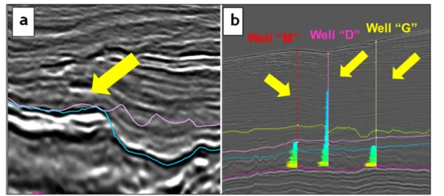
Figure 3 – (a) Seismic section with overlap of unconformities and eroded events pointed by yellow arrow. (b) Seismic section with wells and sonic
profile. Lack of log measurements in the shallow section (pointed by yellow arrow), making it impossible to correlate time to depth, which leaves the velocity from migration as the only available information.
Geostatistics takes into account the geographical location and spatial dependence of the samples (Camargo et al., 1999). As the lateral and horizontal resolutions of the well data and the velocity model are different, the objective is to accommodate these different sources of data to obtain a definition of subsurface in depth reducing the uncertainties.
METHODOLOGY AND PROBLEM INVESTIGATED
This work is a case study from Campos Basin covering an area of approximately 700 km2, in a tectonic environment with erosive
events.
In this work the authors use seven horizons to adjust the velocity model for the time-depth conversion, a PSDM seismic volume and respective velocity imaging (initial model), time-depth tables and seven geological markers referring to the respective interpreted horizons from 17 wells and pseudo-impedance volumes in time.
The geological uncertainties highlighted in this work are the overlap of unconformities and eroded events (Fig. 3a). The lack of log measurements in the shallow section (Fig. 3b), makes it impossible to correlate time to depth, which leaves the velocity from migration as the only available information. Three velocity model scenarios were created: 1) the velocity model of scenario 1 adjusts the horizon interpreted in the seismic section to respective geological markers in the well and influence radius 5 km; 2) the velocity model of scenario 2 uses time-depth table calibration and influence radius 5 km by kriging with external drift; and 3)
the model of scenario 3 uses time-depth table calibration and influence radius 2 km by kriging with external drift.
The criteria for quality control and model validation are: 1) analysis of the conversion of the seismic volumes and pseudo-impedance-P from inversion, comparing the correlations obtained in the conversion to depth in each of the three scenarios and 2) conversion of the time maps to depth and calculating the residuals (δz), adopting the Widess criterion as a parameter Maul et al. (2013). The seismic resolution is calculated from the dominant frequency volume ( fdom) extracted from the seismic
data and the calibrated velocity model (V). From the Widess criterion (Widess, 1973), the vertical seismic resolution is defined by a quarter of wavelength (λ/4) and it is given by Eq. (3). Values of δz≤λ/4 imply errors below the seismic resolution, thus indicating an acceptable result according to the limitation of the seismic method. λ 4 = V 4 fdom , (3) RESULTS
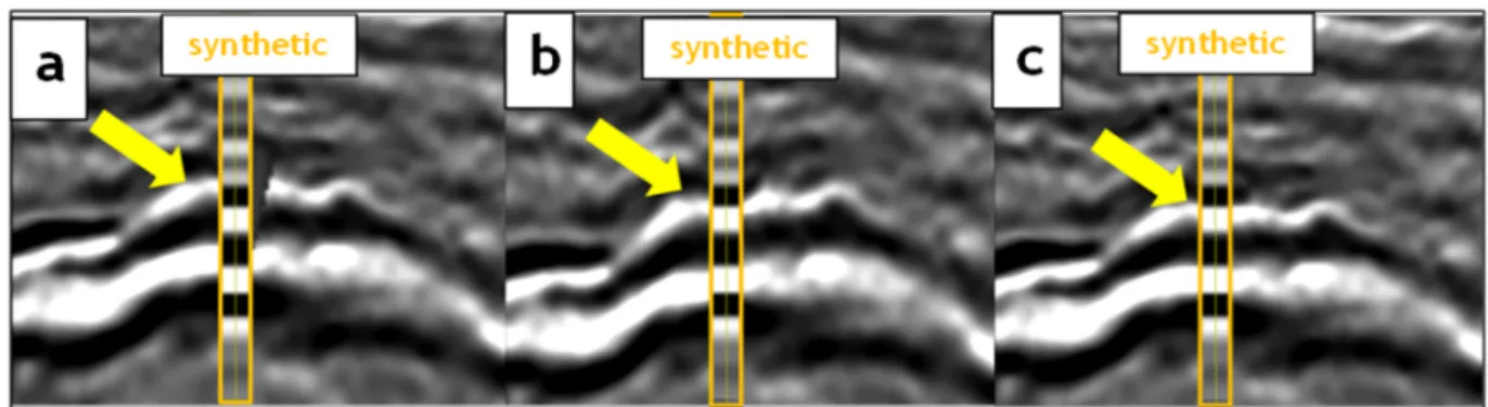
The comparison of the three scenarios shows that scenario 1 presents the best fit between horizon in depth to respective well marker. The Figures 4 and 5 show the synthetic and the seismic section in depth for the three velocity models scenarios. A visual analysis between synthetic and seismic section, the scenario 3 presents best fit (Figs. 4c and 5c) when compared to scenarios 1 (Figs. 4a and 5a) and 2 (Figs. 4b and 5b).
Figure 4 – Synthetic of the well “G” compared to seismic section in depth by the three velocity model scenarios. The white peak in seismic section (pointed by yellow
arrow) presents best fit with synthetic in scenario 3 (c) when compared to scenarios 1 (a) and 2 (b).
Figure 5 – Synthetic of the well “I” compared to seismic section in depth by the three velocity model scenarios. The white peak in seismic section (pointed by yellow
arrow) presents best fit with synthetic in scenario 3 (c) when compared to scenarios 1 (a) and 2 (b).
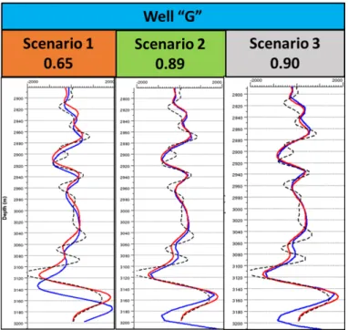
The Figures 6, 7, 8 and 9 present acoustic impedance profiles, obtained from sonic and density logs, shown in black dotted lines, pseudo-impedance extracted from the pseudo-impedance volume at the well positions, converted to depth using the time-depth relationship from each well, displayed in red solid lines, and the pseudo-impedance, also extracted at the wells positions. However, depth-converted using the three different scenarios used to create the three velocity models, shown in blue solid lines.
The correlation between pseudo-impedance logs and impedances values from inversion converted to depth is not preserved in most wells. The Figure 6 shows that well “D” does not have significant changes, i.e. the three scenarios present similar correlation values (0.79, 0.72 and 0.77) between pseudo-impedance Time-Depth conversion with TD table (red line) and pseudo-impedance Time-Depth conversion using the three velocity model scenarios (blue line). In wells “G” (Fig. 7) and “I” (Fig. 8), the correlations between pseudo-impedance Time-Depth conversion with TD table (red line) and pseudo-impedance Time-Depth conversion using
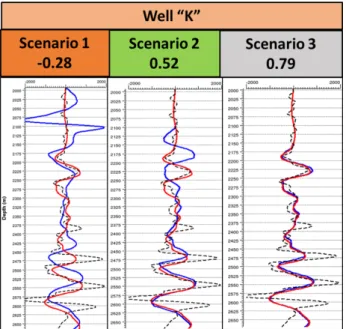
the three velocity model scenarios (blue line) present high correlations in scenarios 2 and 3. The Figure 9 shows well “K”, the correlations are weak in scenarios 1 and 2, where the influence radius in calibration presents strongly influence to these wells.
The scenario 3 is the best for seismic section and horizons time to depth conversion, because it presents: lower horizons-markers residuals values than seismic resolution; best preserves the correlation of pseudo-impedance volumes from the seismic inversion. The table 1 shows the p-impedance volume correlations with the pseudo-impedance obtained from the inversion, converted to depth by the calibrated models with markers and by the tables (Column “Ip Correlation”), the differences of the horizon “H5” (converted to depth by the two models) compared to the respective markers in the wells.
The velocity model in scenario 1 uses well markers, which produces horizons in depth that honor the markers, but implied a velocity model with anomalous values and distortions in seismic depth.
An important aspect to be considered is the loss of time-depth tie with the synthetic seismogram. The depth fit of
Figure 6 – The well “D” with the three scenarios. Acoustic impedance profiles using sonic
and density log (black dotted). The correlation between pseudo-impedance Time-Depth conversion with TD table (red line) and pseudo-impedance Time-Depth conversion using the three velocity model scenarios (blue line) present similar values (0.79, 0.72 and 0.77). Source: Talarico (personal communication, 2016).
Figure 7 – The well “G” with the three scenarios. Acoustic impedance profiles using sonic
and density log (black dotted). The correlation between pseudo-impedance Time-Depth conversion with TD table (red line) and pseudo-impedance Time-Depth conversion using the three velocity model scenarios (blue line) present high correlations in scenarios 2 (0.89) and 3 (0.90). Source: Talarico (personal communication, 2016).
Figure 8 – The well “I” with the three scenarios. Acoustic impedance profiles using
sonic and density log (black dotted). The correlation between pseudo-impedance Time-Depth conversion with TD table (red line) and pseudo-impedance Time-Depth conversion using the three velocity model scenarios (blue line). In the well “I” the correlation is low for scenario 1 and improving substantially in scenarios 2 and 3. Source: Talarico (personal communication, 2016).
Figure 9 – The well “K” with the three scenarios. Acoustic impedance profiles using
sonic and density log (black dotted). The correlation between pseudo-impedance Time-Depth conversion with TD table (red line) and pseudo-impedance Time-Depth conversion using the three velocity model scenarios (blue line) present weak correlations in scenarios 1 (-0.28) and 2 (0.52), where the influence radius in calibration presents strongly influence to these wells. Source: Talarico (personal communication, 2016).
E 0.82 -0.03 5.04 0.70 5.04 25.75 F 0.77 0.69 0.04 0.76 4.83 28.04 G 0.90 0.65 0.03 0.90 11.71 28.24 H 0.84 0.09 1.38 0.71 8.18 25.31 I 0.91 -0.12 0.56 0.91 3.58 31.52 J 0.81 0.59 0.08 0.80 6.31 37.11 K 0.76 -0.28 8.83 0.79 14.93 46.74 L 0.85 0.18 0.10 0.80 10.13 36.81 M 0.66 0.40 0.68 0.47 18.99 30.97
the horizons to the markers presents satisfactory results because horizon-marker residuals values are lower when compared to the seismic resolution defined by Widess criterion (λ/4). However, when analyzing the conversion of the p-pseudo-impedance volumes from the inversion, there is a strong decrease in the correlation with the p-impedance of the wells.
Original Oil in Place Impacts
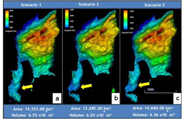
A sensitivity test was performed for the three scenarios and the respective isopachs and structural limits were obtained for a hypothetical area of hydrocarbon accumulation.
The velocity model play an important rule in defining the geological model, which impacts the OOIP (Original Oil In Place) estimates (Eq. 4)
OOIP=A· h · NtG ·φ· (1 − Sw) B0
, (4)
Where:
• OOIP is the volume of Original Oil In Place; • A is the area of the structure;
• h is the thickness of the reservoir;
• NtG is the Net-to-Gross ratio; • φis porosity;
• Sw is the water saturation; • B0the formation volume factor.
The area of an oil accumulation and the reservoir thickness are defined by the geoscientist interpretation using horizon converted from time to depth conversion. In Figure 10 is showed the isopach maps estimates for scenarios 1, 2 and 3.
DISCUSSION AND CONCLUSIONS
The results from the interpretation uncertainties approach with adjust and calibration parameters were the most significant and instructive, showing how subtle changes in the interpretation (seismic horizons) and well markers can lead to unrealistic behavior the horizons in depth. This evidence is supported by the correlation with pseudo-impedance from inversion and synthetic seismogram from well profiles shown on Table 1.
During the time-depth conversion, the disparity in the resulting sections and horizons was remarkable, given the variations in velocity and the initial interpretations of horizons in
Figure 10 – Isopach maps and respective areal structural and rock volume estimates for scenarios 1(a), 2(b) and 3(c). The impact of velocity
model on the reservoir morphology is pointed by the yellow arrow. These differences affect the reservoir thickness and volumes as well.
time. The uncertainties and the sensitivity analysis are sometimes ignored in the context of the exploration. The results of this work show that they are necessary to identify the cause of possible distortions.
The case study shows that, by fully relying on the tying of markers, artifacts and distortions can be created in the time-depth conversion, even if the results are satisfactory.
The seismic interpretation has a influence on the results of the final modeling. Small variations in input data may lead to the generation of non-existent structures and non-geological velocity models results strongly suggest a careful with well logs quality control.
ACKNOWLEDGMENTS
The authors thank Petrobras for allowing publication of this work. The authors thank the manager Francisco Aquino for his support in the publication of the paper. The authors also thank colleagues Raphael Siston, Erick Talarico, Maria Fernanda Barbosa, Luiz Alberto Santos, Fernanda Gobatto and José Eduardo Lira for their ideas, criticism and suggestions. Frank C. Bulhões thanks Bruna Faustino for help and fellowship. The authors thank the VIII Brazilian Symposium on Geophysics commission for
the invitation to publish this work in the Brazilian Journal of Geophysics.
REFERENCES
ANP - Agência Nacional do Petróleo, Gás Natural e Biocombustíveis. 2018. Boletim de Recursos e Reservas de Petróleo e Gás Natural 2017. Available on: <http://www.anp.gov.br/images/DADOS_ESTATISTICOS/ Reservas/Boletim_Reservas_2017.pdf>. Access on: November 3, 2018. BULHÕES FC, AMORIM GAS, BRUNO VL, FERREIRA GD, PEREIRA ES & CASTRO RF. 2014. Fluxo para construção do Modelo de Velocidade Regional da Bacia de Campos. In: VI Simpósio Brasileiro de Geofísica, Porto Alegre. Brazil: SBGf. CD-ROM.
BULHÕES FC, FERREIRA GD & CAPARICA JR JF. 2018. Velocity model calibration: how interpretation uncertainty can impact time-depth conversion. In: Rio Oil & Gas Expo and Conference 2018. Rio de Janeiro, Brazil: Instituto Brasileiro de Petróleo, Gás e Biocombustíveis – IBP. CAMARGO ECG, MONTEIRO AMV, FELGUEIRAS CA & FUKS SD. 1999. Integração de geoestatística e sistemas de informação geográfica: uma necessidade. In: GIS-Brasil 99. 12201. Curitiba, Brazil: Instituto Nacional de Pesquisas Espaciais - INPE.
CRABTREE NJ, ETRIS EL, ENG J, BREWER G & DEWAR J. 2000. Geologically consistent seismic processing velocities improve time to depth conversion. In: Conference Geo-Canada 2000: The Millennium
Recebido em 25 setembro, 2018 / Aceito em 30 outubro, 2018 Received on September 25, 2018 / Accepted on October 30, 2018