Equilibrium Interest Rates in Brazil: A Laubach and
Williams Approach
*Marcelo Fonseca
**Marcelo
Kfoury Muinhos
***Abstract
Real interest rates in Brazil are still high in any international comparison, even considered that they have declined significantly in the last few years. The main purpose of this paper is not only to update but also extend the Laubach and Williams (2003) using fiscal and credit variables. We also present a new methodology to calculate the output gap. Our long run equilibrium rate is slightly above 3% aligned with Laubach and Williams (2003) and supposing long term inflation expectation in US is 2%, real rates there are half what we found for Brazil. Our sensitivity analysis have shown that our results changed slightly in different scenarios regarding Brazil risk premium but deeply to potential GDP growth. Considering the alternative scenario for output gap, real rate values are much lower, because in this case output gap is much wider
Keywords: real interest rate, Laubach Willians, Kalman Filter. JEL Classification: E43, F34.
* We would like to thank Tatiana Nogueira and Natacha Perez for the gathering the data and helping with
the estimations.
** Center of Macroeconomic Studies Macro Brasil FGV-EESP [email protected] *** Professor of Economics and Coordinator of Center of Macroeconomic Studies Macro Brasil FGV-EESP
1- Introduction
After controlling inflation with the launch of the Real plan in 1994, Brazil has not been able to converge to a new steady state with reasonable interest rates. Not only the central bank rate has been above any normal standard consistently in the last 25 years, but also the banking lending rates are even more abnormal.
Nowadays, when we are at the end of the easing cycle, central bank policy rate (Selic rate) is at record low level at 6.50%. Since 2013, the effective real interest rate (discount 12-month inflation expectation) is the lowest, slightly below 3%. Matter of fact, it is not lowest ever; because inflation expectation was higher in 2013, hence real rate was a slightly smaller at that period, as one can see in Table 1. Given there is still idle capacity in the economy, it is possible that the effective rate around 3% is below the equilibrium rate. Hence, two questions that naturally follows: (i) what is the equilibrium rate? (ii) is it the monetary policy accommodative indeed?
Table 1 - Selic and Real Rate
Laubach and Williams (2003) focus their work in estimating the real interest rate – the real interest rate consistent with output equalizing potential and stable inflation – on a medium-run concept of price stability that not considers the effects of short-run price and output fluctuations. Their purpose is to show that the time variation in natural interest rate is important to the analyses and the performance of monetary policy and its real-time mismeasurement can cause a significant deterioration in macroeconomic stabilization.
Based on the definition of the natural rate of interest considering deviation of output from potential, the natural rate of interest estimation also entails finding the
potential output as well. Moreover, giving the linkage between natural interest rate and the trend growth rate, they have to estimate both the level of potential output and its trend growth rate. Therefore, they use Kalman filter to estimate this unobserved variables the potential output trend growth rate. Besides Kalman filter, they model the cyclical dynamics of output and inflation using a restricted VAR model and then, using median-unbiased estimates of these coefficients, based on Stock and Watson (1998), they apply maximum likelihood to estimate the remaining model parameters.
After estimating the model using quarterly U.S. data over the period 1961 to 2000, Laubach and Williams realize an exercise in which they use simulations of the estimated model to assess the effects of natural interest rate mismeasurement. In addition, they found that mismeasurement leads to a significant deterioration in output stabilization but has relatively modest effects on inflation stabilization.
We have analyzed at least five papers with different approaches trying to estimate the real equilibrium interest rate for Brazil. The two papers aiming to measure the equilibrium real interest rate in Brazil with different approaches were Miranda and Muinhos (2002) and Muinhos & Nakane (2006). They performed direct measures from IS curve, panel with different emerging countries, information on the yield curve, even trying to extract the equilibrium rate from marginal productivity. However, using state space in similar fashion as done by Laubach and Williams (2003) was not performed. Barcelos Netto and Portugal (2008) presented the first attempt to calculate the natural interest rates using the Laubach and Williams methodology for Brazil. However, given that the period of estimation ended in 2005, in the first stages of inflation targeting in Brazil, the outcome of the estimation shows a rate hovering 10%, which is significantly greater the what we expect to the range nowadays.
Araujo and Silva (2012) also present some different methodologies of measuring the Brazilian neutral real interest rate: i) statistical filters; ii) a state space macroeconomic model. They include variables such as the real exchange rate, credit default swap and an international interest rate. In the period that they considered, from 2002 up to the end of 2012, they found the country´s natural rate of interest to be around 3.5%.
Perelli Roache (2014) also followed the same approach trying to measure the equilibrium interest rate using statistical filters, short and long run estimation of IS curve micro-founded models and even state space model similar to Goldfajn and Bicalho (2011), but any of the adopted methodologies are not even close to Laubach and Williams (2003).
The purpose of this paper is to not only to update the Laubach Williams (2003) approach for Brazil, but also to include fiscal and credit variables as explanatory variables
in the process. We also add a risk premium variable in the equilibrium interest rate equation and we present a new methodology to calculate the output gap.
We consistently found that equilibrium real interest rate for Brazil is hoovering 4% in the next couple of years.
The following section presents the Laubach Williams methodology and the new variables that we included in the model. In the third session, we present the data and treatment conducted of the exogenous variables. In the fourth, we show our results and some sensitivity analysis. In the fifth section, we summarized and concluded the paper.
2- The Model
We based the approach on Laubach Williams (2003), in which we add some special features to include some characteristics of the Brazilian economy. Following Laubach Williams (2003) and Araujo e Silva (2013), the output gap fluctuations are attributed to real interest gap to a central tendency, which is the real equilibrium rate. In fact, it is not the real interest rate that matters but the difference between the effective real rate and the equilibrium one. It is an augment version of the IS curve in which the dependent variable is the output that depends on the real interest rate gap, on the credit conditions and also on central government expenditures.
ℎ = 𝛽 ℎ + 𝛽 [𝑟 − 𝑠𝑣 + 𝛽 ∆𝐺𝐷𝑃∗ + 𝑟 + 𝐶𝐷𝑆 + 𝛽 𝐹𝐶𝐼 + 𝛽 ∆𝑔 +
𝛽 𝑋 + 𝛽 𝐷 + 𝜀 (1)
𝑠𝑣 = 𝑠𝑣 + 𝜗 (2)
The term inside the brackets is a representation of an interest gap. The neutral rate is the part on the parentheses as shown below.
𝑟∗ = 𝑠𝑣 + 𝛽 ∆𝐺𝐷𝑃∗ + 𝑟 + 𝐶𝐷𝑆 (3)
The first term of equation 3 is the state variable of the system following a very simple ar(1) structure estimated by the Kalman filter. This approach recursively calculates non-observable components using past data. The other terms are the structural part of the equation. The original paper has only the average of potential product growth as a structural variable. For this paper, we include the US interest rate and the Brazilian risk premium measured by the 5 year sovereign credit default swaps (CDS).
𝑟∗ = 𝑠𝑣 + 𝛽 ∆𝐺𝐷𝑃∗ + 𝑟 + 𝐶𝐷𝑆 (4)
3- The Data
Below we explain how we obtained and treated the variables used in our estimations. Output gap (h): our standard measure is calculated as a Hodrick-Prescott filter with a special feature given that the end of the sample period is not the last quarter with data available. We extend our sample up to 2022 using GDP growth Focus consensus forecast. The reason for that is to avoid end-point bias in Hodrick-Prescott estimation.
As an alternative procedure, we use an output gap, which is a weighting average between labor market and industrial capacity utilization slackness as describes in Muinhos and Alves (2003).
Even controlling for the end-point, one can see that the default output gap has a leading recovery comparing to the alternative measure. Both series have a minimum point at -5% at the end of 2016. However, the alternative GDP measure has not recovered significantly in 2017 still presenting an average in comparison to 3% on the default output gap, showing perhaps a premature recovery.
We also included three more alternative output series:
- HiatoIPEA with is a calculated by IPEA using a proper series for potential output based on Cob-Douglas production function.
- Hiato_Gui – a Laubach Willians approached to calculate the output gap as well, done by Guilherme Pazzini, a master student in FGV-EESP
- Hiato 21 similar to the Hodrick-Prescott but with growth at 2.1% from 2020 to 2022.
Figure 2 - Different Output Gaps -.06 -.04 -.02 .00 .02 .04 .06 00 02 04 06 08 10 12 14 16 18 HIATO_GUI HIATO_MKT15 HIATO_MKT21 HIATOIPEA HIATO0619PNAD
Real Rate (r)– it is the Selic rate deflated by 12-month ahead inflation expectation. ∆𝐺𝐷𝑃∗ 4-quarter increasing in our default potential output growth
𝑟 3-month US Treasury rates
𝐶𝐷𝑆 Brazilian risk premium measured by Credit Defaut Swaps (with 5 year mature). The variable used in the estimation is the residual of the risk premium against the output gap to avoid endogeneity.
FCI financial condition index. This variable is year over year household credit growth controlled by output gap and Selic rate as well.
∆𝑔 is the first difference in central government expenditures measured in BRL terms.
4 – Empirical Results 4-1 Estimation Results
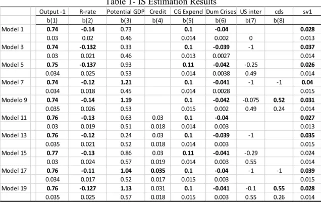
We ran 10 different version of our augmented IS curve. The first one is the closest version to Laubach and Williams (2003). The two extension to the IS curve (credit and central government expenditures) are significant and with the expected sign in all specification as one can see in Table 1. Central government expenditures present the correct sign in all specification, whereas credit is significant at 10% in 4 models and highly significant in Model 17. However, regarding the terms that form the real equilibrium rate (r*) the coefficients that are significant in all the specification is the average of potential output growth and the risk premium. The US interest rates are not significant in any of the specification and the Brazilian risk premium has the correct sign and is statistically significant in the both equation (9 and 19). The state space variable sv1(equation 2) is significant in most of the estimations with coefficient value slightly below the end-point equilibrium real interest rate calculated by equation 3.
Table 1- IS Estimation Results
Source: Centro Macro-Brasil:
Output -1 R-rate Potential GDP Credit CG Expend Dum Crises US inter cds sv1 b(1) b(2) b(3) b(4) b(5) b(6) b(7) b(8) Model 1 0.74 -0.14 0.73 0.1 -0.04 0.028 0.03 0.02 0.46 0.014 0.002 0 0.013 Model 3 0.74 -0.132 0.33 0.1 -0.039 -1 0.037 0.03 0.021 0.46 0.013 0.0027 0.014 Model 5 0.75 -0.137 0.93 0.11 -0.042 -0.25 0.026 0.034 0.025 0.53 0.014 0.0038 0.49 0.014 Model 7 0.74 -0.12 1.21 0.1 -0.041 -1 -1 0.04 0.034 0.018 0.45 0.014 0.0028 0.015 Modelo 9 0.74 -0.14 1.19 0.1 -0.042 -0.075 0.52 0.031 0.035 0.026 0.53 0.015 0.002 0.49 0.24 0.014 Model 11 0.76 -0.13 0.63 0.03 0.1 -0.04 0.027 0.03 0.019 0.51 0.018 0.014 0.003 0.013 Model 13 0.76 -0.12 0.24 0.03 0.1 -0.039 -1 0.035 0.035 0.021 0.52 0.018 0.014 0.003 0.015 Model 15 0.77 -0.13 0.86 0.03 0.11 -0.041 -0.29 0.024 0.03 0.024 0.57 0.019 0.014 0.003 0.55 0.014 Model 17 0.76 -0.11 1.04 0.035 0.1 -0.04 -1 -1 0.039 0.034 0.017 0.52 0.017 0.015 0.003 0.015 Model 19 0.76 -0.127 1.13 0.031 0.1 -0.041 -0.1 0.55 0.028 0.035 0.025 0.57 0.018 0.015 0.003 0.55 0.26 0.014
4.2 - Sensitivity Analysis
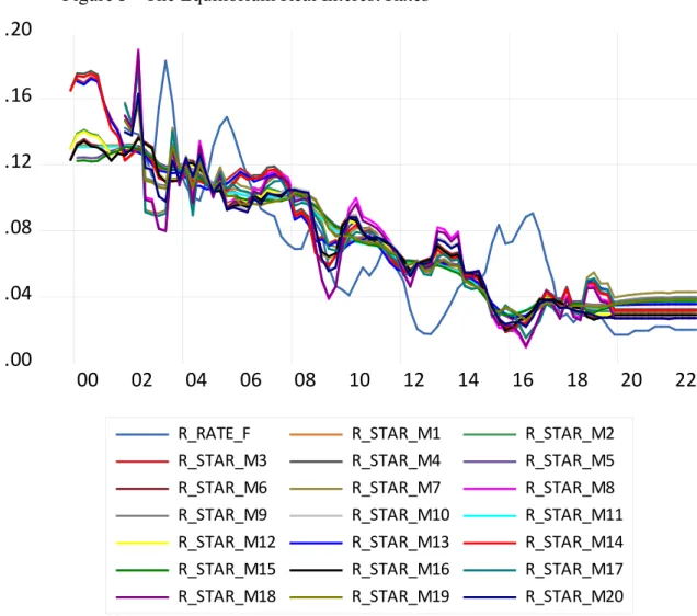
As one can see in Figure 2, our simulations of the real equilibrium rate converges to an average of 3.3% in the last quarter of 2022. The graphical representation is distributed in a close range from 2.7% in Model 8 up to 4.1% in Model 5. It is worth noticing that 2018 average about 3.4% is similar to the average in 2022. Hence, according to our estimation Brazil is running nowadays an expansionary monetary policy but only about 200 bps below neutral.
Figure 3 - The Equilibrium Real Interest Rates
.00 .04 .08 .12 .16 .20 00 02 04 06 08 10 12 14 16 18 20 22
R_RATE_F R_STAR_M1 R_STAR_M2
R_STAR_M3 R_STAR_M4 R_STAR_M5
R_STAR_M6 R_STAR_M7 R_STAR_M8
R_STAR_M9 R_STAR_M10 R_STAR_M11
R_STAR_M12 R_STAR_M13 R_STAR_M14
R_STAR_M15 R_STAR_M16 R_STAR_M17
R_STAR_M18 R_STAR_M19 R_STAR_M20
The terminal conditions matter regarding the variables that we consider exogenous in our simulation. Hence, in the situation that we called normal condition, we considered CDS at 170 bps and GDP growth at 1.3%.
Table 2
Based on that, we consider some sensitivity analysis in our simulation. In the case of a worsening of the international condition our hypotheses is that CDS moves gradually to 300 in the end of the horizon. In this case, the real equilibrium rate will reach 3.8% in average and 4.4% in Model 19. On the other hand, in case of CDS getting lower reaching 100 in 2021; real equilibrium rate also decreases to 3% in average and 3.2% in the model 19.
The sensitivity analysis for GDP growth is more puzzling, and it potential GDP. Considering another measure of output gap, the equilibrium interest rates are significantly smaller. Our alternative GDP measure has a negative level of 0% in average in 2019 in comparison to 3% on the default output gap. The equilibrium real rate is 0.7% when we used the alternative output gap. Another problem using this alternative rate is only the autoregressive and real rate (b2) coefficients are significantly different from zero.
Equilibrium Real Interest Rate
Average Model 19
2019Q3 2022Q4 2019Q3 2022Q4
Normal 3.5 3.3 3.4 3.8
High CDS 3.9 3.8 3.8 4.4
Low CDS 3.3 3 3.1 3.2
Hiato IPEA 0 0.5 neg neg
Hiato Pnad 0.7 0.7 0.3 0.6
Hiato_gui 3.5 3.6 2.9 3.8
7- Conclusions
Real interest rates in Brazil are still high in any international comparison, even considered that they have declined significantly in the last few years. The main purpose of this paper was not only to update but also extend the Laubach and Williams (2003) using fiscal and credit variables. Indeed the effective rate around 3% is below the equilibrium rate and the monetary policy is slightly accommodative, given we found equilibrium rate in 2018 at 3.3% in average.
Regarding IS estimation, results presented in Table 1 shows most of the coefficients estimated for Brazil are significant and with the expected sign with the only exception of the US interest rates, which is not different from zero in any estimation.
Our long run equilibrium rate is slightly above 3%, with is in line with the results for Laubach and Williams (2003), however, we use real interest rate in our estimation and they used nominal interest rate. Hence supposing long-term inflation expectation in US is 2%, real rates there are half what we found for Brazil.
Our sensitivity analysis have shown that our results changed slightly for different scenarios for Brazil risk premium but deeply in regards to potential GDP growth. Considering the alternative scenario for output gap, real rate values are much lower, because in this case output gap is much wider.
Two possible extensions of this paper are: (i) to include in our estimation other Latin American countries that use inflation targeting as the monetary policy framework such as Peru, Chile, Colombia and Mexico. (ii) to use the output gap as a state variable as well, so the system would be a multivariate Kalman filter with two state space equation: real interest rate and output gap.
7- References
Araújo, Rafael C. and Silva, Cleomar G. da (2014): “The Neutral Interest Rate and the Stance of Monetary Policy in Brazil”. Procedings of the 41st Brazilian
Economics Meeting 051, ANPEC.
Barcelos Netto and Portugal (2008) “The Natural Rate of Interest in Brazil between 1999 and 2005, Revista Brasileira de Economia 63(2) p103-118
Goldfajn, Ilan, and Aurelio Bicalho. (2011) “A longa travessia para a normalidade: os juros reais no Brasil.” Texto para discussão Itau Unibanco 2.
Laubach, T and Williams, J. C.(2003): “Measuring the Natural Rate of Interest”, The Review of Economics and Statistics, Vol. 85, No. 4, pp. 1063-1070.
Miranda, Pedro and Muinhos, M. K. (2003): “A taxa de juros de equilíbrio: uma abordagem múltipla”, BCB Working Paper Series 66.
Muinhos, Marcelo and Nakane Marcio (2006): Comparing equilibrium interest rates: stylized facts about Brazilian figures BCB Working Paper Series 101
Muinhos, Marcelo and Alves Sergio “Medium-Size Macroeconomic Model for the Brazilian Economy" Economia Aplicada, Vol. 7, n. 1, (Jan-Mar 2003).
Perrelli, Roberto and Shaun K. Roache. (2014) “Time-Varying Neutral Interest Rate-the Case of Brazil.” IMF Working Papers 14/84
Stock, J. and Watson, M. (1998): “Median Unbiased Estimation of Coefficient Variance in a Time Varying Parameter Model”, Journal of the American Statistical Association, Vol 93, pp. 349-358.