Comparing equilibrium real interest rates: different
approaches to measure Brazilian rates
*Marcelo
Kfoury Muinhos
**Márcio I. Nakane
***Abstract
Despite the difficulties involved in the precise determination of equilibrium real interest rates, it seems clear that nominal interest rates has been higher in Brazil than in similar emerging economies. This paper aims to shed light on the possible reasons for this feature of the Brazilian economy. We extend Miranda and Muinhos (2003) one-country study to a sample of 20 countries, using many methods to compare measures of the real interest: (i) extracting equilibrium interest rates from IS curves; (ii) extracting steady state interest rates from marginal product of capital; (iii) capturing relevant variables and the fixed effects having real interest rates as dependent variable in a panel for emerging countries; and (iv) extracting inflation expectation from the spread between fixed rate and inflation-indexed treasure notes.
Keywords: real interest rate, marginal product of capital, IS curve. JEL Classification: E43, F34.
*
We wish to thank Afonso Sant'Ana Bevilaqua, José Pedro R. Fachada Martins da Silva and Carlos Hamilton Vasconcelos Araújo for useful comments and suggestions. Marcelo Yoshio Takami helped to extract inflation risk from fixed and inflation-indexed treasure notes. We are also indebted with Erica Diniz Oliveira and Ibitisan Borges Santos as research assistants. The views expressed are those of the authors and not necessarily those of the Central Bank of Brazil.
**
Research Department, Banco Central do Brasil. E-mail: [email protected]
***
1- Introduction
After taming inflation with the launching of the Real plan in 1994, Brazil is still in the process of converging real interest rates to a level comparable to other countries. After the Real plan, an exchange rate anchor was implemented, and in consequence high real interest rates were required to adjust the balance of payments in face of external shocks. After 1999, an inflation targeting cum flexible exchange rate enabled a reduction in real interest rates. Nevertheless, as one can see in Table 1 where all developed countries and even most of emerging countries have been able to reduce real interest rates to levels around 3%, Brazil rates in the 2000-2004 period is still close to two digits but it also show significant reduction since the previous period.
Some experts blame the fiscal consolidation with high debt service costs, the memories of the near hyperinflation period or even more fundamental reasons like the inter-temporal rate of substitution or the marginal product of capital for the high real interest rates. The reasons have not been exhaustively studied, though.
In particular, Favero and Giavazzi (2002) appointed the macroeconomic fundamentals and the perverse debt dynamics as the reasons for the high level of the yield curve. Arida, Bacha and Lara-Resende (2004) created a vague term, jurisdictional uncertainty, which enhances the original sin hypothesis1 as the main culprit. For the authors, currency inconvertibility, artificial lengthening of public debt maturities, compulsory saving funds and distorting taxation are public interventions that disturbed even more the jurisdiction uncertainty.
Gonçalves et al. (2005) tested Arida, Bacha and Lara-Resende conjecture in a panel data of 50 countries and found no support for it. They included proxies for jurisdictional uncertainty as well as for currency inconvertibility alongside inflation and public debt-to-GDP ratio in a regression for short-term real interest rates. While the last set of control variables proved to be significant in their estimations, the same could not be found for the jurisdictional uncertainty and currency inconvertibility measures.
Another possible explanation is related to the existence of some path-dependence due to the fact that Brazil has a past history of serial sovereign defaults in the sense of Reinhart et al. (2003) [see also Reinhart and Rogoff (2004)]. The authors identify country clusters (clubs) according to both a proxy for default risk (the Institutional Investor ratings) and to total external debt-to-GNP ratios. One interesting finding is that the debt-to-GNP thresholds for serial defaulters are much lower than for non-defaulters. In other terms, despite high debt-to-GNP ratios, non-defaulters have low default risk. As for the serial defaulters, debt-to-GNP ratios have lower trigger defaults. Brazil is included in the club of ‘debt intolerant’ countries and, although Brazil last external debt servicing difficulties occurred in 1983, the effects on the country’s Institutional Investor rating have been long lasting. Previous to the 1983 default, Brazil had ratings close to the ‘non-defaulter’ group. Brazilian ratings after 1983 have not yet been back to such levels.
1
The purpose of this paper is to extend Miranda and Muinhos (2003) analysis for Brazil in terms of regional comparisons. The goal is not only measuring equilibrium real interest rates with different approaches for emerging markets, but also to explore possible reasons for the apparent Brazilian puzzle.
Periods Total Range 1960-64 1965-69 1970-74 1975-79 1980-84 1985-89 1990-94 1995-99 2000-04
Developed
Countries 1.8363 1.18 1.49 -1.23 -1.68 2.22 4.78 5.09 2.84
G7 1.84 1.61 1.70 -1.04 -1.85 2.98 4.68 4.13 2.53
German 2.05 0.88 1.61 1.91 -1.45 3.28 3.51 4.34 2.09 2.27
Canadá 3.04 ND ND ND -0.18 3.29 5.25 4.14 2.92 2.80
USA 2.28 1.64 1.98 0.91 -0.87 4.49 4.38 2.56 2.95 2.52
France 1.83 0.03 1.96 0.56 -3.37 1.88 4.71 6.12 2.73(98-)
Italy 2.41 ND 2.98(69) -0.97 -2.39 2.10 6.23 5.87 3.72 1.75
Japan 1.47 3.91 1.62 -2.43 -0.66 3.52 3.47 2.84 0.11 0.88
United Kingdown 0.48 ND =-1.43(69) -6.24 -7.56 2.31 5.64 4.36 3.24 3.52
Others
Australia 2.04 ND ND -2.23 -2.82 2.03 6.14 5.18 3.96
Austria 1.84 ND 1.15(67-) -0.56 0.26 2.56 3.31 4.26 1.93
Belgium 1.61 0.82 0.15 -1.24 -1.08 2.75 4.04 5.20 2.21
Dinamark 3.74 ND ND .1.02(72-) 1.80 4.75 5.03 7.74 2.11
Spain 1.15 ND ND -4.66(74) -5.27 2.23 5.72 6.29 2.88 0.88
Holand 1.98 -0.20 0.69 -1.12 -0.58 2.85 5.04 4.79 1.30
Ireland 2.01 ND ND -1.44(71-) -1.74 0.61 6.50 7.70 2.80 -0.33
New Zeland 5.95 ND ND ND ND 6.72(78-) 5.76 5.88 5.45
Portugal -0.58 ND ND ND -5.29(78-) -6.96 1.95 4.56 2.83
--Sweden 2.50 ND 3.21(66-) -1.44 -1.37 2.05 5.05 6.00 4.47 2.02
Period Averages 1960-64 1965-69 1970-74 1975-79 1980-84 1985-89 1990-94 1995-99 2000-04 Emerging
Countries 0.33 0.17 -4.32 0.89 3.23 4.44 4.72 3.78 Southeast Asia 2.60 ND 3.76(68-) -5.87 0.66 3.41 4.89 2.40 4.12
South Korea 4.75 ND ND ND 3.98(77-) 3.50 5.73 6.52 6.88 1.33
Honk Kong -3.29 ND ND -6.89(74) ND ND ND -4.38(91-) 1.50
--Indonesia 1.69 ND 3.76(68-) -3.19 -3.26 2.99 5.59** 3.01 6.99 1.54
Malasya 1.71 ND ND -0.37 0.61 3.20 2.86 2.46 1.50
Singapure 1.48 ND ND -5.39(72-) 2.80 4.00 3.92 1.11 2.39 1.52
Thailand 3.88 ND ND ND 2.00(77-) 5.96 5.98 3.91 4.53 0.90
Latin American 8.99 ND ND ND ND 6.50 9.12 15.80 4.54
Argentina 19.59 ND ND ND ND 18.66 21.10 31.56 7.04 9.54
Brazil 11.38 ND ND ND ND 7.54(81-) 5.72 13.06 20.55 9.25
Colombia 6.23 ND ND ND ND ND ND ND 6.23 0.84
Mexico 0.84 ND ND ND ND -15.15(82-) -0.45 6.62 5.46 4.51
Uruguay -0.12 ND ND ND ND ND ND -3.40(94) 3.17
--Venezuela -20.17 ND ND ND ND ND ND ND -20.17(96-) 3.56
Others
South Africa 0.74 1.25 1.18 -2.15 -4.03 -0.28 -1.19 1.66 7.05 3.66
India 1.44 1.51 -5.18 0.67 8.87 -2.75 2.10 4.65 1.67
--Poland 8.25 ND ND ND ND ND ND -7.87(91-) 5.50 7.44
Russia 0.16 ND ND ND ND ND ND ND 23.80 3.30
Source: International Finance Statistics -IMF
Real Interest Rates for Selected Countries
2- The natural rate of interest in Emerging Countries: concepts and measures
Wicksell described the natural rate of interest in at least three dimensions: -(1) the rate of interest that equates savings with investment;
-(2) the marginal productivity of capital;
-(3) the rate of interest that is consistent with aggregate price stability.
A more recent definition that is common in the New-Keynesian models with stick prices defines the natural rate as the one that balances a rational expectation dynamic model with flexible prices.
A direct and simple way to calculate equilibrium rates is to filter ex-post real interest rates of high frequency movements to avoid transitory shocks to the economy. Borio et al (2000) suggested the use of a Hodrick-Prescott filter with a very high parameter λ to smooth the trend series.
Our results for a sample of 18 countries from 1992 to 2002 are displayed in Figure 1. We calculate ex-post real interest rates using again data from the International Finance Statistics from IMF to obtain nominal interest rates, and deflating with the 12 month accumulated inflation rate. Table 2 presents the averages of equilibrium real interest rates for the whole period and three sub periods for the emerging countries divided in three regions. Latin American country averages are the greatest for all the periods. Brazil's numbers are the second highest in the whole sample with only Peru displaying higher figures. However, the trend is downward during the analyzed period. Chile, Colombia and Mexico have a pattern similar to East Asia countries. East Europe is the only region where the averages show increases in the most recent period.
A second measure of natural real interest rates is potential output growth. Many central banks use this measure as a rule of thumb. Our measure of the potential output is a linear trend on the GDP series for all the countries. The output for each country is regressed against individual coefficients for the time trend and for seasonal dummies, and potential output growth is the annualized time trend for each country.
Figure 1 Actual and Filtered Real Interest Rates -.3 -.2 -.1 .0 .1 .2 .3 .4 .5
95 96 97 98 99 00 01 02 03 04 LREALINT__ARG LREALINTHP_ARG_ .05 .10 .15 .20 .25 .30
96 97 98 99 00 01 02 03 04 LREALINT__BRA LREALINT9504_BRA_ -.04 .00 .04 .08 .12 .16
93 94 95 96 97 98 99 00 01 02 03 04 LREALINT__CHI LREALINTHP_CHI_ -.04 .00 .04 .08 .12 .16
96 97 98 99 00 01 02 03 04 LREALINT__COL LREALINTHP_COL_ -.05 .00 .05 .10 .15 .20 .25
95 96 97 98 99 00 01 02 03 04 LREALINT__CRO LREALINTHP_CRO_ .00 .04 .08 .12 .16 .20
95 96 97 98 99 00 01 02 03 LREALINT__CZE LREALINTHP_CZE -.6 -.5 -.4 -.3 -.2 -.1 .0 .1 .2 .3
94 95 96 97 98 99 00 01 02 03 LREALINT__ECU LREALINTHP_ECU_ -.4 -.3 -.2 -.1 .0 .1
94 95 96 97 98 99 00 01 02 03 LREALINT__EST LREALINTHP_EST_ -.02 .00 .02 .04 .06 .08 .10
94 95 96 97 98 99 00 01 02 LREALINT__HUN LREALINTHP_HUN_ -.2 -.1 .0 .1 .2 .3
94 95 96 97 98 99 00 01 02 03 LREALINT__IND LREALINTHP_IND -.02 .00 .02 .04 .06 .08 .10 .12 .14
92 93 94 95 96 97 98 99 00 01 02 03 LREALINT__KOR LREALINTHP_KOR_ -.08 -.04 .00 .04 .08 .12
93 94 95 96 97 98 99 00 01 02 03 LREALINT__LAT LREALINTHP_LAT -.3 -.2 -.1 .0 .1 .2
94 95 96 97 98 99 00 01 02 03 LREALINT__LIT LREALINTHP_LIT_ -.1 .0 .1 .2 .3 .4 .5 .6
93 94 95 96 97 98 99 00 01 02 03 LREALINT__MEX LREALINTHP_MEX_ .10 .15 .20 .25 .30 .35
93 94 95 96 97 98 99 00 01 02 03 LREALINT__PER LREALINTHP_PER_ -.02 .00 .02 .04 .06 .08 .10 .12 .14
92 93 94 95 96 97 98 99 00 01 02 03 LREALINT__PHI LREALINTHP_PHI_ -.02 .00 .02 .04 .06 .08 .10 .12
92 93 94 95 96 97 98 99 00 01 02 03 LREALINT__THA LREALINTHP_THA -.4 -.2 .0 .2 .4 .6 .8
Period Average Total 1990-94 1995-99 2000-04 Emerging
Countries 4.27 5.70 4.60 4.70
Southeast Asia 4.00 4.65 5.10 2.25
Korea 4.80 7.10 6.00 1.60
Indonesia 4.00 2.50 5.70 2.90 Philippines 4.80 5.90 4.90 4.00 Thailand 2.50 3.10 3.80 0.50
Latin America 8.40 12.85 9.00 7.50 Argentina* 4.40 3.24 6.20 7.60 Brazil 12.40 22.00 15.20 10.00
Chile 4.10 3.40 5.70 2.70
Colombia 3.80 ND 5.40 1.80 Mexico 5.70 6.60 6.20 4.10
Ecuador 6.00 -18.00
Peru 20.00 29.00 18.30 16.70
East Europe 0.40 -0.38 -0.20 2.47
Croatia 4.90 na 8.30 0.60
Czech 2.40 1.00 3.00 1.90
Estonia -6.50 na -8.00 2.10 Latvia 0.00 0.40 -1.00 1.00 Lithuania -0.30 -2.11 -1.50 2.90 Turkey 1.90 -0.80 -2.00 6.30 * Data until 2002
Equilibrium Real Interest Rate Table 2
Period Average Total 1992-98 1999-02 Emerging
Countries 2.95 4.24 4.50
Southeast Asia 2.53 5.50 4.24* 5.67
Korea 5.20 6.60 8.30
Indonesia -0.50 na -0.05 Philippines 3.70 4.40 4.90 Thailand 1.70 5.50 3.80
Latin America 2.60 3.93 2.2* 3.23 Argentina 0.75 4.00 -4.00
Brazil 3.04 4.00 2.90
Chile 4.80 6.70 3.80
Colombia 1.20 2.70 1.90
Mexico 3.00 2.00 4.40
Ecuador 1.20 2.40 3.80
Peru 3.90 5.70 2.60
East Europe 3.73 3.29 4.60 Croatia 3.20 3.57 3.40
Czech 1.60 3.10 2.50
Estonia 5.10 4.10 5.80
Latvia 5.40 2.70 7.90
Lithuania 3.20 1.99 4.14
Turkey 2.94 4.30 3.95
* Including Indonesia and Argentina
3- Results from IS equations
Another possibility to obtain equilibrium real interest rate measures is to compute the interest rate that eliminates the output gap. This computation can be obtained from an IS equation.
g = f(g-t, r, x)
From which, we find: 0 = f(0, r*, x)
where g is the output gap and x represents a set of other explanatory variables.
The IS equations were estimated for the 17 countries in our sample. The estimated equation is:
gt =γ0 + γ1gt-1 + γ2(it-1-πt-1) + γ3(Expt-1) + γ4(logcapt-1) + γ5D1t + γ6D2t + γ7D3t + ηt (1) where g is the output gap, i is the nominal money rate, π is the accumulated 12 months inflation, exp is the log of exports and, logcap is the log of capital inflow to the country, and D1, D2 e D3 are seasonal dummies.
One can calculate the equilibrium real interest rate by the equation:
2 6 5
0 exp log
*
γ γ γ
γ D t capt
r =− + + + (2)
where D is the average of the seasonal coefficients.
Period Average Total 1998-02
Emerging Countries
Southeast Asia
Korea 9.02 7.20
Indonesia -8.36 -70.00
Philippines -97.00 0.36
Thailand 2.93 -48.00
Latin America 7.58 10.91
Argentina 4.80 -100.00
Brazil 11.11 13.04
Chile 0.72 5.88
Colombia 2.36 0.14
Mexico 7.49 5.64
Ecuador 138.00 21.71
Peru 19.00 19.03
East Europe -4.60 3.43
Croatia -14.17 3.40
Czech 1.17 2.50
Estonia -11.17 5.50
Hungary 8.24 6.24
Latvia -1.80 2.02
Lithuania -9.67 0.94
Real Interest Coefficient in the IS Curve Table 4
4- Marginal Product of Capital
Another way to gather information on real interest rates for particular countries is to have a measure of the marginal productivity of capital. Different economic models suggest that the equilibrium real interest rate should be close to the real return on capital, a measure of which is the marginal productivity of capital.
In this section, we report two measures of marginal product of capital for Brazil. The first measure is the gross marginal product of capital while the second one is a net measure after taking into account any wedge created by inefficiencies.
The gross marginal product of capital comes from Ferreira, Pessôa and Veloso (2005). The starting point for the calculation is a Cobb-Douglas production function of the form
(
)
−αα
= 1
it it it it
it K A L H
Y
where Yit is the output of country i at time t, K is physical capital, H is human capital per worker, L is raw labor and A is labor-augmenting productivity and α is the capital share in output. In this economy, gross marginal product of capital is given by:
it it MgPK Gross
κ α =
In order to calculate the capital-output ratio, Ferreira, Pessôa and Veloso (2004) use data on output per worker and investment rates obtained from the Penn-World Tables, version 6.1 for a sample of 83 countries for the period 1960-2000. We only report the results for the year 2000. The physical capital series is constructed using the Perpetual Inventory Method. Depreciation rate is assumed to be the same for all economies, and obtained from US data, being equivalent to 3.5% per year. The parameter α is also the same for all economies, and it is taken to be equal to 0.4, a figure close to the capital income share of the US economy according to the National Income and Product Accounts (NIPA).
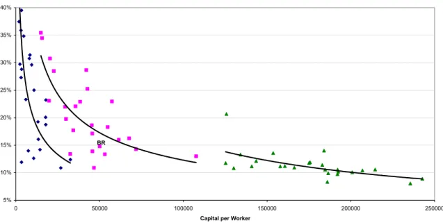
Figure 2 shows the results of the calculation for a sample of 75 countries with available data. The sample is split in three groups according to the level of income per worker. For each income group, countries are ranked according to the level of capital per worker.
Figure 2
Gross Marginal Product of Capital (%)
5% 10% 15% 20% 25% 30% 35% 40%
0 50000 100000 150000 200000 250000
Capital per Worker BR
Brazil is included in the intermediate income group. Within this group, the gross marginal product of capital for Brazil (15%) is below a fitted polynomial for the sub-sample of intermediate-income countries.
The gross marginal product of capital may not give a precise account of the return to capital because countries may differ in the efficiency with which the capital stock is employed. We then adjust the gross measures by taking into account any wedge created due to inefficiencies arising from rent-seeking activities. We borrow from Barelli and Pessôa (2002)’s two-sector framework where rent-seeking activities are modeled as diverted output from the productive sector. Under the assumption that both sectors operate with the same Cobb-Douglas technology, net marginal product of capital is given by:
( )
θ R βit it
it it
l 1
MgPK Gross
MgPK Net
where θ is part of the argument of a function g describing the share of the output of the productive sector that is extracted by the unproductive sector; this function has (θyR) as its argument where yR is the ratio of output of the unproductive sector to the output of the productive sector. The term θ has the interpretation of describing the quality of the institutional set. A high (low) θ represents a bad (good) institutional background. lR is the ratio of workers employed in the rent-seeking sector to workers employed in the productive sector, and β is a parameter that appears in the specific functional form used for the g function, which is the following:
β β
+ =
x x x g
1 ) (
Barelli and Pessôa (2002) use a measure of institutional quality created by Hall and Jones (1999) to calibrate θ for each country. We adopt the same procedure but replace the measure of institutional quality of Hall and Jones by the Corruptions Perception Index compiled by International Transparency. We took the country scores for 2000. For β, which is assumed to be the same for all countries, we take the value calibrated by Barelli and Pessôa (2002), setting it to 0.506.
The relative allocation of workers between the unproductive and productive sectors (lR) is calibrated in two steps. First, from the World Bank Investment Climate Surveys, we take the answers to the question “Percent of management time dealing with officials” as our measure of labor share allocated to rent-seeking activities. World Bank reports the mean answers for 46 developing countries. The intersection of countries in the World Bank survey and in the Penn World Tables is very small, with only 16 countries but, luckily, Brazil is one of them.2
For the other countries we take the World Bank’s Doing Business Project. In special, we use the answers to the following items: “days and number of procedures to start up a business”, “days and number of procedures to enforce a contract”, and “time and number of procedures to register property”. We then run a regression for the 43 countries for which there is data on both sets of World Bank surveys. The dependent variable is (log of) “percent of management time dealing with officials”. The explanatory variables are the levels of the six variables in the Doing Business Survey, plus their squares and cross products. The coefficient of determination (R2) for this regression is 57.4%. What we want to do is to use the fitted regression to “forecast” the “percent of management time dealing with officials” for the countries in the Penn World Tables for which we cannot directly observe this variable. The forecasted variable is then taken to be our measure of labor share allocated to rent-seeking activities for these countries.
Figure 3 shows the estimates for the net marginal product of capital for a sample of 64 countries with available data. The sample is split in three groups according to the level of income per worker. For each income group, countries are ranked according to the level of capital per worker.
2
Figure 3
Net Marginal Product of Capital (%)
5% 7% 9% 11% 13% 15% 17% 19% 21% 23% 25%
0 50000 100000 150000 200000 250000
Capital per worker BR
The net marginal product of capital for Brazil is estimated to be 10%. Such value is consistent with real interest rate measures observed for Brazil according to the alternative methodologies described in the other sections of this paper. However one cannot observe any remarkable difference between Brazil and the other countries using this methodology, as it was possible to notice in the previous sections of this paper. The net marginal productivity of capital seems to go some way towards explaining the level of Brazilian rates but not the difference in relative terms for other countries.
Table 5 shows the estimates for the both the gross and net marginal product of capital for some selected countries alongside the values for capital and income per worker.
Gross Marg Prod of Capital
Net Marg Prod of Capital
Capital per Worker
Income per Worker
Emerging Countries
Southeast Asia
Korea 11.77% 7.62% 125,261 36,850
Indonesia 20.10% 9.67% 17,803 8,944 Malaysia 16.26% 12.26% 67,674 27,507 Philippines 18.74% 11.28% 17,874 8,374 Thailand 10.90% 7.28% 46,629 12,702
Latin America
Argentina 14.30% 8.58% 71,798 25,670
Brazil 14.79% 10.06% 50,078 19,220
Chile 18.30% 15.12% 54,826 25,084
Colombia 23.10% 13.15% 19,876 11,477
Ecuador 13.41% 6.98% 32,524 10,903
Mexico 16.01% 9.99% 61,450 24,588
Peru 12.39% 7.98% 32,583 10,095
Venezuela 13.36% 6.95% 53,146 17,754 Table 5
5- Real Interest Rates, Fiscal Debt and Risk Premium.
Favero and Giavazzi (2002) argued that interest rates are high in Brasil due to the level of debt service, among other reasons. In this section our goal is to compare real interest rates in emerging countries with debt/GDP ratio and also with risk premium.
We could not find a clear connection between debt/GDP ratio with our HP filtered real interest rates. One could expect that countries with high debt/GDP ratio would have to pay higher interest rates to roll over their debts. But only for Argentina, Brazil, Philippines and Turkey, as one can note in Table 6, there is a positive correlation between these variables for the whole period, which weakens the proposed relationship. Table 6 also shows that for shorter samples it was also possible to obtain positive correlation for Colombia, Czech Republic and Indonesia. But for the case of Brazil, a Granger causality test does not show that debt “causes” real interest rates (Table 8). In almost all other cases even when the correlation is negative, one can reject the null of no Granger causality in both directions (Tables 7 and 8).
Full Sample 1995-2004
Correlation Correlation Period Southeast Asia
Korea -78.17%
Indonesia -77.35% 12.97% 1995:1 - 1999:3 Philippines 56.96%
Thailand -97.65%
Latin America
Argentina 71.79% 90.47% 1995:1 - 2001:2 Brazil 70.40%
Chile -91.01%
Colombia -90.28% 94.84% 1995:1 - 1998:2 Mexico -93.89%
Peru -73.22%
Europe
Czech -68.57% 46.45% 1995:1 - 1998:4 Turkey 93.03%
Table 6
Filtered Real Interest Rate and Debt-GDP Ratio: Correlation Coefficients
Obs F-Statistic Probability
Southeast Asia
Korea 36 3.44 4.49% Indonesia 28 2.31 12.16% Philippines 31 2.68 8.76% Thailand 36 8.12 0.15%
Latin America
Argentina 26 2.15 14.09% Brazil 34 8.36 0.14% Chile 28 4.65 2.02% Colombia 34 3.29 5.16% Mexico 36 2.09 14.13% Peru 32 1.80 18.43%
Europe
Czech 36 5.47 0.92% Turkey 36 5.98 0.64%
Table 7
Filtered Real Interest Rate and Debt-GDP Ratio: Granger Causality Tests
Null Hypothesis: Interest Rate does not Granger cause Debt-GDP
Obs F-Statistic Probability
Southeast Asia
Korea 36 5.49 0.91% Indonesia 28 5.73 0.96% Philippines 31 29.30 2.20E-07 Thailand 36 0.14 87.28%
Latin America
Argentina 26 11.92 0.04% Brazil 34 0.89 42.13% Chile 28 2.76 8.43% Colombia 34 5.37 1.04% Mexico 36 26.22 2.20E-07 Peru 32 269.64 1.40E-18
Europe
Czech 36 9.15 0.08% Turkey 36 15.55 2.10E-05
Table 8
Filtered Real Interest Rate and Debt-GDP Ratio: Granger Causality Tests
Null Hypothesis: Debt-GDP does not Granger cause Interest Rate
effects are significant for almost all countries and the point estimate coefficient for Brazil is consistent with other estimations of equilibrium real interest rates, being the second highest in the sample.
Table 9
Dependent Variable: Log Real Interest Rate
Estimation Method: Seemingly Unrelated Regression Sample: 1995Q1 2003Q4
Included observations: 36
Linear estimation after one-step weighting matrix
Coefficients t statistic p value
Lrealint(-1) 0.518751 21.50193 0
D(Debtpib) -0.05718 -3.22417 0.0014
Res 1.34E-18 0.298514 0.7655
Excr -2.56E-07 -1.35198 0.1771
Fixed effects
Arg – c 0.032955 2.320683 0.0208
Bra – c 0.072822 4.664381 0
Chi – c 0.019079 4.562541 0
Col – c 0.02988 4.527892 0
Cze – c 0.013992 3.121617 0.0019
Ind – c 0.028204 2.601458 0.0096
Kor – c 0.020101 5.808784 0
Mex – c 0.026046 1.984372 0.0479
Per – c 0.081557 13.78672 0
Phi – c 0.021262 6.434374 0
Tha – c 0.01274 3.479943 0.006
Tur – c 0.011723 0.380456 0.7038
Favero and Giavazzi (2002) concluded that macroeconomic fundamentals and debt dynamics are the main determinants of the term spread of Brazilian rates during the period of 1999 to 2002. In our panel, we related the debt/GDP ratio with a proxy of the equilibrium real interest rate for various emerging markets and the relationship was not the one obtained by Favero and Giavazzi. A better variable to explain the debt dynamics is the Embi risk premium, which takes into account not only the path of the debt/GDP ratio but also other considerations about debt sustainability. A similar panel with the first difference of the Embi spreads replacing debt/GDP ratio found a positive and significant relationship, as we would expect (Table 10). The fixed effect term is lower than before but it is still the second highest in the sample.
Table 10
Dependent Variable: Log Real Interest Rate
Sample: 1996Q1 2004Q1 Included observations: 33
Total system (unbalanced) observations 326 Linear estimation after one-step weighting matrix
Coefficients t statistic p value
Lrealint(-1) 0.796019 25.70261 0
D(embi) 0.300547 3.085892 0.0022
Excr -0.000052 -1.88119 0.0609
Fixed effects
Arg – c 0.946522 0.601231 0.5481
Bra – c 2.475459 3.16881 0.0017
Bul – c -6.01381 -0.84008 0.4015
Col – c 0.023901 0.06377 0.9492
Ecu – c -2.15593 -1.19683 0.2323
Kor – c 0.146685 0.285856 0.7752
Mex – c 0.931182 2.41139 0.0165
Phi – c 1.008595 2.83168 0.0049
Pol – c 1.333755 4.515269 0
Tur – c 4.51907 1.014414 0.3112
Ven – c -2.73606 -1.64445 0.1011
The correlation between real interest rates and country risk can also be observed in Figure 4 where country ratings from Moody’s are displayed against real interest rates. One can observe a (weak) negative correlation between the rating and interest rates.
Figure 4 – Real Interest Rates and Moody’s Ratings
Cro
Tha Kor
Lat Arg Ind
Bra Per
Cze Chi
Lit
Est Tur
Mex
-8 0 8 16 24
SD Ca Caa3 Caa2 Caa1 B4 B2 B1 Ba3 Ba2 Ba2 Baa3 Baa3 Baa1 A3 A2 A1 Aa3 Aa2 Aa1 Aaaa
Moody's Rating
R
eal
I
n
te
rest
R
a
te
Col Phi
6- Inflation risk and inflation expectation from the Government Bonds
Comparing ex-ante interest rates and ex-post interest rates can give us a measure of inflation risk. Figure 5 shows this data for Brazil, Mexico, Chile and Colombia.3 Only for these four countries we were able to obtain a time-series of inflation expectations, so we restricted the comparison among them. One can see that for Brazil there was a significant difference between the two rates in 2002. The average ex-ante rate in 2002 was 16.20% while the ex-post rate was 7.8%, less than half. For the whole analyzed period the average ex-ante rate was 14.11% and the ex-post was 10.85%, being the average inflation surprise of around 2.9%. This difference shrinks considerably in the more recent period, with the ex-ante rate being higher than the ex-post rate in the first semester of 2004 (i.e, expected inflation was above actual inflation in the period). In
3
Mexico, the ex-post rate was around 1% smaller than the ex-ante in the second half of 2003 and in Chile the ex-post rate is greater than the ex-ante during the sample (that is, there was a “disinflation surprise”). In Colombia from 2003 onwards the ex-ante rate is 3.51% and the ex-post a little higher (4.45%)
Figure 5 - Ex ante and Ex-post Interest rates in Brazil, Mexico and Chile
BRAZIL: real interest rate (% a.a.) - November/01 to May/05
1.00% 6.00% 11.00% 16.00% 21.00%
Nov-01 Jun-02 Jan-03 Jul-03 Feb-04 Aug-04 Mar-05
ex ante ex post
MEXICO: real interest rate (% a.a.) - November/01 to May/05
0.00% 1.00% 2.00% 3.00% 4.00% 5.00% 6.00%
Nov-01 Jun-02 Jan-03 Jul-03 Feb-04 Aug-04 Mar-05
CHILE:real interest rate (% a.a.) - November/01 to April/05
-1.50% -0.50% 0.50% 1.50% 2.50% 3.50%
Nov-01 Jun-02 Jan-03 Jul-03 Feb-04 Aug-04 Mar-05
ex ante ex post
COLOMBIA: real interest rate (%a.a.) -November/03 to July/04
2.00% 2.50% 3.00% 3.50% 4.00% 4.50% 5.00% 5.50% 6.00%
01-09-03 21-10-03 10-12-03 29-01-04 19-03-04 08-05-04 27-06-04
ex ante ex post
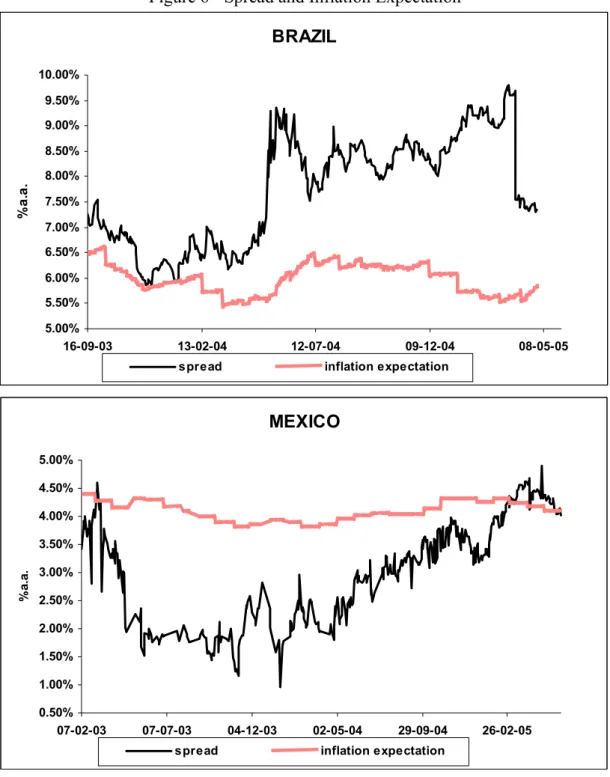
Another way to capture the inflation risk is through the difference between fixed and inflation-indexed government bonds for similar maturities. The spread between the two rates contains an inflation expectation term and a risk premium term.
Fixed rate note= real interest rate + inflation expectation + inflation premium Inflation-indexed rate note = real interest rate + liquidity premium
spread = inflation expectation + premium
premium = inflation premium – liquidity premium
It is possible to estimate the premium by using market consensus inflation expectations. But it is not possible to disentangle inflation and liquidity premiums. Figure 6 shows the spread and inflation expectation one year ahead for Brazil, Mexico, Chile and Colombia.4 From May 2004 to March 2005, the premium was around 2.5% in Brazil
4
while it was close to zero in Mexico in 2003 and around –3.0% in Chile in the whole sample. In Colombia there is no large difference between these two series. Only for Brazil the inflation premium is higher than the liquidity premium. It may suggest that investors are still ensuring themselves against inflation surprises in Brazil, despite the recent fall in inflation
Figure 6 - Spread and Inflation Expectation
BRAZIL
5.00% 5.50% 6.00% 6.50% 7.00% 7.50% 8.00% 8.50% 9.00% 9.50% 10.00%
16-09-03 13-02-04 12-07-04 09-12-04 08-05-05
%a
.a
.
spread inflation expectation
MEXICO
0.50% 1.00% 1.50% 2.00% 2.50% 3.00% 3.50% 4.00% 4.50% 5.00%
07-02-03 07-07-03 04-12-03 02-05-04 29-09-04 26-02-05
%a
.a
.
spread inflation expectation
CHILE
-2.00% -1.00% 0.00% 1.00% 2.00% 3.00%
05-11-02 04-04-03 01-09-03 29-01-04 27-06-04 24-11-04 23-04-05
%a
.a
.
spread inflation expectation
COLOMBIA
3.00% 4.00% 5.00% 6.00% 7.00% 8.00%
02/09/2003 02/01/2004 02/05/2004 02/09/2004 02/01/2005 02/05/2005
%a
.a
.
7- Conclusions
Real interest rates in Brazil are higher than in other emerging economies. The main purpose of this paper was to document such outlying behavior for the Brazilian interest rates through the use of different methodologies.
We provide estimates for equilibrium real interest rates in Brazil and in some selected emerging countries according to the following methodologies: HP filtered series, growth of potential output, rate consistent with zero output gap (IS model), marginal product of capital, and fixed effect of panel regressions after accounting for risk premium and inflation risk through fixed and inflation indexed Treasure Bonds.
The measures are roughly consistent across the different methodologies and most of them point to the behavior of real interest rates in Brazil mentioned above. The paper does not have the purpose of providing definite answers to such stylized facts. However, some elements that emerged from our analysis and may prove useful as potential avenues to explore in future work.
The institutional quality creates a wedge between gross and net returns and may be related to the jurisdictional uncertainty as stressed by Arida et al. (2004). The net marginal productivity of capital explains the level of Brasil real interest rate but not the difference in relative terms for other countries. Such uncertainty raises the country risk premium as documented in our panel regressions. However, risk premium is not the whole story. Even after accounting for this factor, the fixed effects show that there is still some element in the Brazilian rates to be explained.
The last section sheds some light on the effect of inflation risk on real interest rates in Brazil. For 2002, ex-ante interest rates was twice higher than ex-post rates, meaning that inflation risk may have a role in explaining the level of ex-ante real interest rates in Brazil.
8- References
Arida, P., Bacha, E,. Lara-Resende A. (2004): “Credit, interest and jurisdictional uncertainty: Conjectures for the case of Brazil”, mimeo.
Barelli, P., Pessôa, S. A. (2002): “A model of capital accumulation and rent-seeking”, mimeo.
Borio, C., English W., and Filardo A. (2002): “A tale of two perspectives: old or new challenges for monetary policy”, BIS Working Paper nº 127.
Favero, C., Giavazzi F. (2002): “Why are Brazil's interest rate so high?”, Innoncenxo Gasparini Institute for Economic Research Working Paper nº 224.
Ferreira, P. C., Pessôa, S. A., Veloso, F. A. (2005): “The evolution of international output differences (1960-2000): from factors to productivity”, mimeo.
Hall, R., and Jones, C. (1999): “Why do some countries produce so much more output per worker than others?”, Quarterly Journal of Economics, 114, 83-116.
Miranda, P. and Muinhos, M. K. (2003): “A taxa de juros de equilíbrio: uma abordagem múltipla”, BCB Working Paper Series 66.
Reinhart, C. M., Rogoff, K. S., Savastano, M. A. (2003): “Debt intolerance”, Brookings Papers on Economic Activity, (1), 1-74.