Title
Estimating the age and mechanism of boulder transport related with extreme waves using lichenometry
Abbreviated short title
Linking extreme waves, coastal boulders and lichenometry
Authors
Maria A Oliveira1,2,*, Esteve Llop3, César Andrade2,4, Cristina Branquinho1, Ronald Goble5,
Sónia Queiroz2, Maria C Freitas2,4 and Pedro Pinho1
Affiliations and corresponding address
1 Centre for Ecology, Evolution and Environmental Changes, Faculdade de Ciências da
Universidade de Lisboa, Portugal
2 Instituto Dom Luiz, Faculdade de Ciências da Universidade de Lisboa, Portugal 3 Department of Evolutive Biology, Ecology and Environmental Sciences - Botany and
Mycology, Universitat de Barcelona, Faculty of Biology, Spain
4 Departamento de Geologia, Faculdade de Ciências da Universidade de Lisboa, Portugal 5 Department of Earth and Atmospheric Sciences, University of Nebraska-Lincoln, United
States of America
*corresponding author. Email: maoliveira@fc.ul.pt
Acknowledgements
The authors would like to acknowledge João Nuno Silva and Mariana Ramos for field work assistance and Paulo Henriques, geologist in the Portuguese National Authority for Civil Protection, for information and photographic record of rock-falls in the Ericeira region.
Maria A Oliveira was funded by FCT (Fundação para a Ciência e Tecnologia) through a PhD scholarship (SFRH/BD/66017/2009). The work undertaken was partially supported by IDL through UID/GEO/50019/2013 program, financed by FCT; and also partially funded by European project NitroPortugal: Strengthening Portuguese research and innovation capacities in the field of excess reactive nitrogen (EU H2020-TWINN-2015 692331). Pedro Pinho was financed by project H2020 BiodivERsA32015104.
This research is framed within the College on Polar and Extreme Environments (Polar2E) of the University of Lisbon.
For Peer Review
Estimating the age and mechanism of boulder transport related with extreme waves using lichenometry
Journal: Progress in Physical Geography Manuscript ID PPG-19-107.R2
Manuscript Type: Main Article
Keywords: rocky coastline, limestone, optically stimulated luminescence, Portugal, frequency
Abstract:
Tsunamis and storms cause considerable coastal flooding, numerous fatalities, destruction of structures, and erosion. The characterization of energy and frequency associated with each wave contributes to the risk assessment in coastal regions. Coastal boulder deposits represent a physical proof of extreme inundation and allow us to study the effects of marine floods further back in time than instrumental and historical records. Age estimation of these deposits is challenging due to lack of materials (such as sand, shells, corals, or organic matter) that retain information about the passage of time. Lichenometry, a simple age estimation method, cost-effective, quick to apply, and non-destructive, is here proposed as a solution. A lichen growth model for a
calcium-tolerant lichen species was developed and used to estimate the age of a boulder deposit related to extreme marine inundation(s) in Portugal. Estimated ages indicate several very recent events (<700 years) for most of the boulders’ stabilization and agree with results obtained with optically stimulated luminescence of marine sands found beneath boulders. Frequent and recent boulder transport implies a storm-origin for this deposit. These conclusions contrast with other works describing identical deposits and attributed to palaeotsunamis. This study presents a methodology using lichenometry as a successful alternative for age estimation in rocky coastal settings. These results offer an alternative explanation for coastal boulder deposits found on the west coast of Portugal.
For Peer Review
1 Title2
3 Estimating the age and mechanism of boulder transport related with extreme waves using 4 lichenometry
5
6 Abbreviated short title 7
8 Linking extreme waves, coastal boulders and lichenometry 9
10 Abstract 11
12 Tsunamis and storms cause considerable coastal flooding, numerous fatalities, destruction of 13 structures, and erosion. The characterization of energy and frequency associated with each wave 14 contributes to the risk assessment in coastal regions. Coastal boulder deposits represent a physical 15 proof of extreme inundation and allow us to study the effects of marine floods further back in 16 time than instrumental and historical records. Age estimation of these deposits is challenging due 17 to lack of materials (such as sand, shells, corals, or organic matter) that retain information about 18 the passage of time. Lichenometry, a simple age estimation method, cost-effective, quick to apply, 19 and non-destructive, is here proposed as a solution. A lichen growth model for a calcium-tolerant 20 lichen species was developed and used to estimate the age of a boulder deposit related to extreme 21 marine inundation(s) in Portugal. Estimated ages indicate several very recent events (<700 years) 22 for most of the boulders’ stabilization and agree with results obtained with optically stimulated 23 luminescence of marine sands found beneath boulders. Frequent and recent boulder transport 24 implies a storm-origin for this deposit. These conclusions contrast with other works describing 25 identical deposits and attributed to palaeotsunamis. This study presents a methodology using 26 lichenometry as a successful alternative for age estimation in rocky coastal settings. These results 27 offer an alternative explanation for coastal boulder deposits found on the west coast of Portugal. 28
29 Keywords: 30
31 Rocky coastline, limestone, frequency, optically stimulated luminescence, Portugal 32
33
Introduction
34
35 Age estimation of sediments is crucial in geosciences, in cases allowing validation or rejection of 36 conceptual models. In this context, age-estimation is a powerful tool for reconstructing the 37 chronology and return period of extreme marine inundations, which is relevant for coastal hazards 38 and risk assessment (Marriner et al., 2017). In what concerns coastal boulder deposits, this is a 39 challenging task due to a lack of materials that retain information about the passage of time since 3 4 5 6 7 8 9 10 11 12 13 14 15 16 17 18 19 20 21 22 23 24 25 26 27 28 29 30 31 32 33 34 35 36 37 38 39 40 41 42 43 44 45 46 47 48 49 50 51 52 53 54 55 56 57 58 59
For Peer Review
41 tsunami events in boulder accumulations is no trivial task and a highly debated issue (Marriner et 42 al., 2017; Cox et al., 2018; Vött et al., 2019). This distinction is especially relevant when 43 addressing coastal areas with a high risk of tsunami inundation, such as Portugal (cf. Muir-Wood 44 and Mignan, 2009), as both events are characterized by different return periods (decades for 45 extreme storms and centuries to millennia for tsunamis).
46
47 Chronology of onshore boulder movement by waves can be obtained with radiocarbon ages of 48 biogenic calcium carbonate attached to or beneath boulders (Jones and Hunter, 1992; Nott, 2000; 49 1997; Hall et al., 2006; Mastronuzzi et al., 2007; Susuki et al., 2008; Scheffers et al., 2009; Costa 50 et al., 2011; Rixhon et al., 2018; Schneider et al., 2019), by electron spin resonance dating of coral 51 boulders (Scheffers et a., 2014) and by uranium-series radiometric age dating (Scheffers et al., 52 2014; Terry et al., 2016; Remy et al., 2018). Moreover, optically stimulated luminesce (OSL) 53 dating of sand has been used to constrict the age of boulder deposition (Hall et al., 2006; Kennedy 54 et al., 2007). Another possibility is cosmogenic nuclide build-up applied to rock samples taken 55 from exposed horizontal surfaces. However, this method has limitations in what concerns rock 56 thickness (>0.5m for limestone rocks) and increased uncertainties in rocky coastline contexts and 57 boulder deposits (cf. Masarik and Wieler, 2003; Darvil, 2013; Hurst et al., 2017; Trenhaile, 2018). 58 Regardless, cosmogenic 3He or 36Cl age estimation was successfully applied to large boulders
59 attributed to extreme marine events (Ramalho et al., 2015; Rixhon et al., 2018). When materials 60 suitable for age estimation are not available, alternative methods must be considered. In this 61 context, lichenometry stands out as a possible dating methodology of rock surface exposure 62 (including boulder surfaces).
63
64 Lichens are a symbiosis between an algae or cyanobacteria and fungi that maintain their 65 morphology and grow very slowly. This feature has allowed its use in lichenometry, which rests 66 on the relationship between lichen size and age (Beschel, 1961; McCarthy, 1999). If the growth 67 of a lichen species is known, the time elapsed since exposure and stabilization of a rock surface 68 can be inferred from the size of lichens. Lichens with concentric growth have been widely used 69 since the 60s to estimate the age of recent glacial and periglacial deposits (e.g., Carrara and 70 Andrews, 1975; Birkeland, 1982; Proctor, 1983; O’Neal and Schoenenberger, 2003; Orwin et al., 71 2008; Hansen, 2008; Roberts et al., 2010; Trenbirth and Matthews, 2010; Roof and Werner, 2011; 72 Rosenwinkel et al., 2015; Garibotti and Villalba, 2017; Pendleton et al., 2017). Furthermore, 73 lichenometry was applied to rockfall debris (McCarrol et al., 2001; Bull, 2014), debris-flow 74 deposits (Innes, 1983; Jonasson et al., 1991), coble and boulder beaches in coastal regions 75 (Broadbent and Bergqvist, 1986) and fluvial deposits (Gob et al., 2003; Foulds et al., 2014). 76
77 Absolute age estimation using lichenometry requires control points (i.e., substrates with a known 78 age of exposure) and a function correlating the size of lichens with time, referred to as a growth 79 curve (Innes, 1985; Armstrong, 2004). This curve must be built for a given lichen species (or 80 genus) and environmental conditions in which the deposits or surfaces to be dated occur. In the 81 absence of control points, a growth-rate curve can also be built by monitoring the growth of lichen 82 thalli of different sizes, and by assuming a direct relationship between lichen size and age 83 (Armstrong, 2015). Lichenometry is mostly useful for dating the past 500 years, its upper limit of 84 applicability being determined by senescence and competition among individuals (Beschel, 1961; 85 Innes, 1985; Noller and Locke, 2000; Armstrong, 2004).
3 4 5 6 7 8 9 10 11 12 13 14 15 16 17 18 19 20 21 22 23 24 25 26 27 28 29 30 31 32 33 34 35 36 37 38 39 40 41 42 43 44 45 46 47 48 49 50 51 52 53 54 55 56 57 58
For Peer Review
87 Lichenometry has been contested by several authors due to methodological issues and sources of 88 errors (Jochimsen, 1973; Worsley, 1990; McCarthy, 1999; Jomelli et al., 2007; Osborn et al., 89 2015; Decaulne, 2016). Arguments against the technique include the unknown influence of 90 ecological variables in lichen growth; factors related with population dynamics, such as lichen 91 competition, mortality and rapid population turnover; inheritance of older lichens from previously 92 exposed rocks; sampling techniques, including between-operator variance, the use of lichen 93 diameter in elongated thalli, and the number of thalli sampled; lichen identification in the field; 94 and the lack of uncertainty or statistical validity.
95
96 Some of the drawbacks of this technique can be overcome by sampling in microhabitats showing 97 optimal lichen growth (McCarthy, 1999; Trenbirth and Matthews, 2010; Decaulne, 2016). 98 Decadal and century-scale climate change affecting lichen growth rates can be incorporated by 99 using indirectly established lichen growth curves (Innes, 1985; Armstrong, 2015). Changes in 100 growth rates due to competition can be avoided by using only isolated thalli. Highly dynamic 101 populations are not a problem if life-cycle processes are similar in sampled surfaces (Armstrong, 102 2016), which can be checked by monitoring lichen growth and mortality (Decaulne, 2016). 103 Inheritance can be detected with systematic sampling coupled with statistical analysis based on 104 the variance of lichen size (Rosenwinkel et al., 2015). Between-operator variance can be resolved 105 with all measurements being taken by the same person (Innes, 1985). Irregular thalli can be 106 measured as surface area based on photographic record (Worsley, 1990; Roof and Werner, 2011). 107 Issues related to the limited number of individuals measured by using the largest thalli or the five 108 largest thalli colonizing a surface can be resolved by using a size-frequency approach (Bradwell, 109 2004). The correct identification of lichen species is an inevitable necessity to minimize sources 110 of error, and it can be resolved by collaborating with taxonomists (Decaulne, 2016). Finally, by 111 using available statistical software (such as R), statistical uncertainty can be included in 112 predictions.
113
114 Regardless of all the uncontrolled factors, the large number of successful and reproducible results, 115 indicates that lichen size is a reasonable measure of the age of a geological deposit (Innes, 1985). 116 Although rare, studies of lichen growth in calcareous substrates exist (Trudgill et al., 1979; Maas 117 and Macklin, 2002). However, applications to rocky substrates exposed to the harsh coastal 118 environment are few, and comprise the use of this technique as a relative age estimator (cf. 119 Williams and Hall, 2004).
120
121 In this work, we show an innovative approach to the chronology of coastal boulder emplacement 122 by extreme marine events in rocky limestone coastal contexts, by using lichenometry, combined 123 with OSL. A calibration curve, including uncertainty, was developed using lichens in control 124 points with known age, including man-made masonry structures in coastal forts and rock-scars 125 from slope mass movements. The growth curve was used to constrain the age of emplacement of 126 limestone boulders in a coastal deposit. The lichen species Opegrapha durieui Mont. (Roux and 127 Egea, 1992) was used for this purpose. By estimating the age of boulder deposition, we aim to 128 clarify the origin (tsunami vs. storm) of the boulder accumulation in a region with a high risk of 129 tsunami inundation. The approach presented herein can be applied to other coastal contexts 130 elsewhere, provided that local control points are used for model calibration, and that sampling 131 strategies take into consideration lichen species ecology.
132 3 4 5 6 7 8 9 10 11 12 13 14 15 16 17 18 19 20 21 22 23 24 25 26 27 28 29 30 31 32 33 34 35 36 37 38 39 40 41 42 43 44 45 46 47 48 49 50 51 52 53 54 55 56 57 58 59
For Peer Review
133Study area
134
135 Boulder deposit 136
137 The boulder deposit is located on the west coast of Portugal, approximately 40km NW of Lisbon 138 (Figure 1a). Tides are semidiurnal, and considering one Saros cycle, the highest astronomical 139 spring tide reaches 1.8m amsl (above mean sea level); the mean spring tidal range is 2.8m 140 (Instituto Hidrográfico, 1985-2003). Layers outcropping in the study area comprise uplifted 141 marine transgressive-regressive sequences deposited during the lower Cretaceous (Rey, 2007). 142 The sequence is slightly dipping to SW (6-10°) and formed by alternating crystalline limestone 143 to sandy limestone layers at the base (Units A-D), followed by claystone, sandstone, and marl 144 (Unit E) (Figure 1b-c). The basal sequence (Units B-D) forms wide ramps, benches with 145 protruding limestone layers, and low vertical cliffs (<20m). These evolve by rock-fall due to 146 breakdown along bench and cliff edges, forming boulders with varying sizes reflecting bed 147 thickness and joint spacing. Wide structural platforms develop between each unit, forming 148 benches up to 3 m high. Marl, sandstone, and mudstone layers outcropping at the top of the 149 sequence (Unit E) form low-sloping cliffs that evolve by gullying and mass movement, generating 150 colluvium. Limestone layers from units C and D differ from each other in their composition 151 (ranging from crystalline to sandy limestone), in fossil content, surface morphology, thickness, 152 and joint frequency and direction (Oliveira, 2017).
153
154 [insert Figure 1.]
155 Figure 1: a) Location of the study area in Europe and Portugal; (b) geological units (A-E), 156 location of cross-sections (CS1-3) represented in Figure S1 in SM (Supplementary Materials), 157 and insets represented in Figure 2a and b; (c) schematic log of the units
158
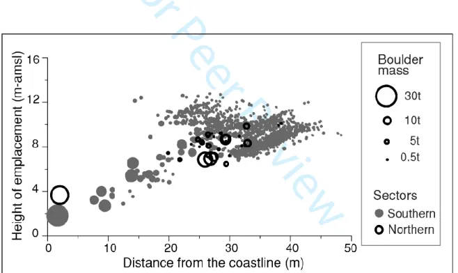
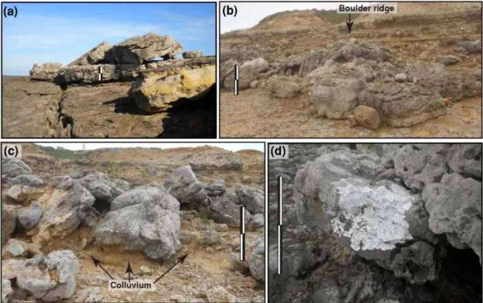
159 The deposit comprises 1500 supratidal limestone boulders up to 30 tons at 2-13 m amsl, both 160 north and south of Coxos beach, on top of the structural surfaces formed by Units C and D (Figure 161 2a-b). Only boulders showing evidence of transport against gravity were addressed in this study. 162 Boulders sitting on top of Unit C were sourced in layers 17-19, and boulders sitting on top of unit 163 D were sourced in layers 20-28 (Figure 1c). Transported particles originated in overhanging or 164 notched limestone layers exposed to storm wave swash, some of them having been overturned 165 and broken during transport. Boulders show a landward and northward size-grading trend, 166 decreasing in size as the elevation increases, in agreement with the general slope of the structural 167 surface (Figure 2a-b and Figure S2 in SM). Larger boulders (>10ton) are generally located inland 168 of natural indentations in the lower structural platform, and either lean against bench edges or sit 169 horizontally and isolated, close to the edge of the benches (Figure 2a-b and Figure S3a in SM). 170 Further inland, closer to the inner edge of the structural platforms, boulders are smaller (<2.5ton). 171 They are organized in ridges and clusters of imbricated boulders (Figure 2a-b and Figure S3b in 172 SM). In the southern sector, the development of colluvium deposits partially buries some of the 173 boulders (Figure S3c in SM). Isolated boulders found near the edge of the cliffs/benches, are 174 sometimes close to sockets matching their size, and interpreted has their original location. 3 4 5 6 7 8 9 10 11 12 13 14 15 16 17 18 19 20 21 22 23 24 25 26 27 28 29 30 31 32 33 34 35 36 37 38 39 40 41 42 43 44 45 46 47 48 49 50 51 52 53 54 55 56 57 58
For Peer Review
176177 [insert Figure 2.]
178 Figure 2: (a) and (b) boulders’ mass north and south of Coxos beach; (c), (d), (e) boulders 179 colonized by the lichen species Opegrapha durieui.
180
181 The lichen species Opegrapha durieui colonized 32 boulders forming ridges and imbricated 182 clusters and in an isolated boulder on top of a cliff at 12 m amsl (Figure 2c-e and Figure S3d in 183 SM). Boulders colonized by lichens within clusters were surrounded by many other large clasts 184 but lacking colonization by this lichen species.
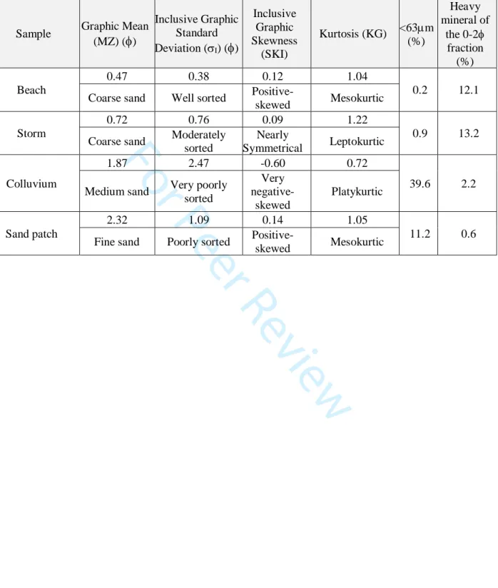
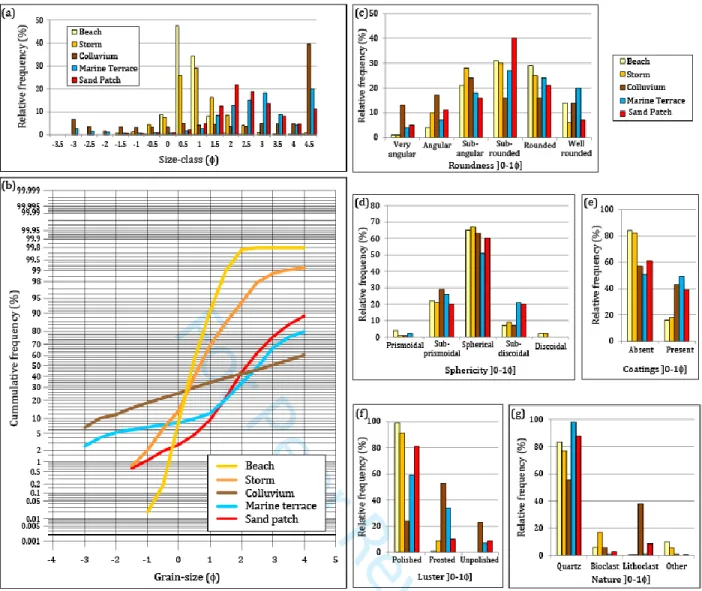
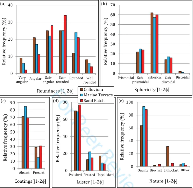
185 Boulder movement up to 12m amsl was observed in the study area in January and February of 186 2014. However, the inner part of the ridges with boulders colonized by lichens remained generally 187 untouched. A patch of marine sand was found beneath boulders within a ridge, at 9m amsl (Figure 188 3). Before the storms, this material was covered by boulders and colluvium. The marine sand 189 patch comprised a poorly sorted fine sand with a bimodal distribution, containing sub-rounded 190 coated, clean and polished quartz grains, lithoclast, and bioclasts (Oliveira, 2017). Grain size, 191 morphology, composition, and morphoscopic surface features of the quartz grains contrast with 192 material from the beach, the colluvium deposit and from sand collected in the lower rocky 193 platform after storms (cf. Oliveira, 2017) (data shown in Table S1 and Figures S4-S5 in SM). 194
195 [insert Figure 3.]
196 Figure 3: a) Front view of the bolder ridge and exposed sand patch beneath the boulders (1m 197 scale); b) Sampling for OSL age estimation
198
199 Lichen Species on boulders at Coxos deposit 200
201 Opegrapha durieui is a slow-growing and circular species, and therefore an excellent candidate 202 to be used in geochronology (Innes, 1985; Noller and Locke, 2000). Lichen species with 203 Trentepohliam as photobiont, such as Opegrapha durieui, are more abundant in humid and warm 204 conditions, common in tropical and subtropical regions (Sipman and Harris, 1989; Nimis and 205 Tretiach, 1995). There is a positive relationship between Trentepohlia lichen richness and 206 temperature (van Herk et al., 2002; Aptroot and van Herk, 2007; Marini et al., 2011). Moreover, 207 lichens with Trenrepohlia are most frost susceptible than species containing other photobionts, 208 such as Trebouxia or Nostoc (Nash et al., 1987). The development of lichens with Trentepohlia 209 is linked to high levels of moisture and precipitation, being more abundant in rainy and oceanic 210 areas (Rindi and Guiry, 2002; Marini et al., 2011).
211
212 Opegrapha durieui colonizes calcareous rocks in the supra-littoral fringe subject to sea spray, in 213 the Mediterranean and adjacent Atlantic coasts of Morocco and Portugal, where humid-warm 214 climates dominate (Roux and Egea, 1992; Sipman and Raus, 1999; Nimis, 2016). Lichen thalli 215 are generally found in very steep to vertical, and overhanging humid cliff faces looking North, 216 (Nimis, 2016), and are absent in near-horizontal dry surfaces with high exposure to sunlight (Roux 3 4 5 6 7 8 9 10 11 12 13 14 15 16 17 18 19 20 21 22 23 24 25 26 27 28 29 30 31 32 33 34 35 36 37 38 39 40 41 42 43 44 45 46 47 48 49 50 51 52 53 54 55 56 57 58 59
For Peer Review
218 its distribution to a thin strip in the coastal area (<50-75m inland from the sea). On the one hand, 219 this species does not tolerate frequent and direct seawater and is not found close to the direct 220 effect of sea spray, this niche being occupied by other lichen species. On the other hand, it is 221 rarely found away from the coastline. These taxa bound to maritime-coastal situations (Nimis, 222 2016). The restricted ecology of this lichen species assures that sites where it is found share 223 similar ecological/climatic conditions.
224
225 Opegrapha durieui forms white, thin, continuous to cracked and areolate epilithic thalli, with a 226 white prothallus. Apothecia are lirellated, almost immersed in the thallus, black with a whitish 227 pruina, simple to irregularly branched and 1-2mm-long (Figure 4). When two thalli coalesce, one 228 of two things occurs: the more competitive thallus overgrows the weakest, which eventually dies, 229 or they form a contact boundary and keep colonizing surrounding areas. These boundaries form 230 perceptible, thick, linear, and segmented features (Figure 4).
231
232 [insert Figure 4.]
233 Figure 4: Coalescing thalli of Opegrapha durieui 234
235
Methods
236
237 Selection of control points 238
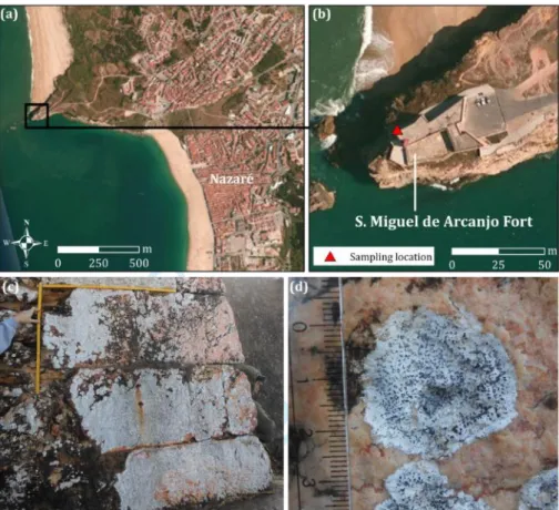
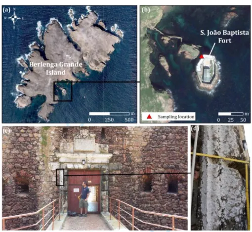
239 The calibration curve was based on data from 14 control points located along the Portuguese coast 240 (detailed description in SM) (Figure 5). Surfaces include shelly, clastic to crystalline limestone, 241 and concrete. Although these materials show different physical, mineralogical, textural, and 242 chemical characteristics, they all contain calcium carbonate in high proportions, which controls 243 the pH of the substrate. Control points include selected man-made masonry structures found in 244 coastal forts and other artificial structures, and recent (<70 years) scars from slope mass 245 movements.
246
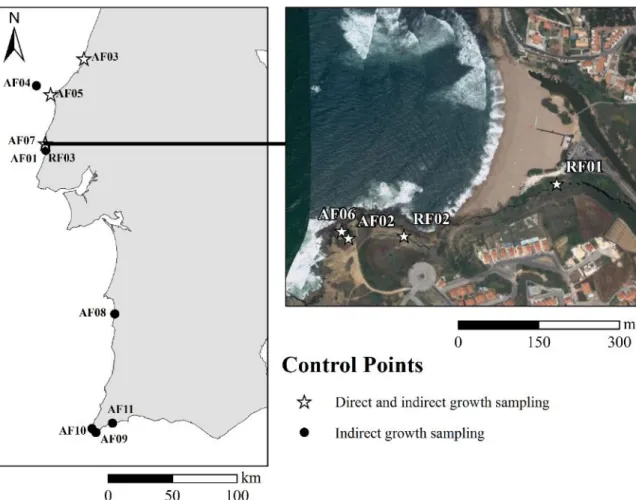
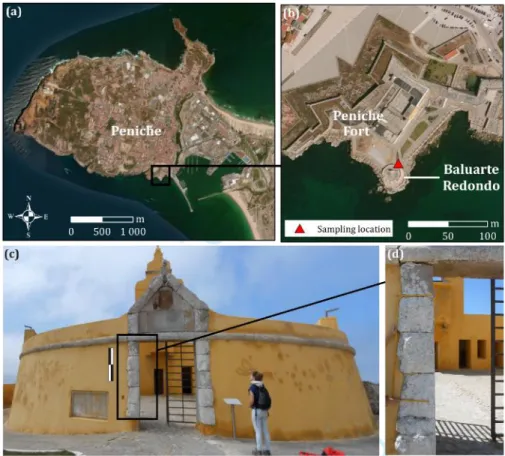
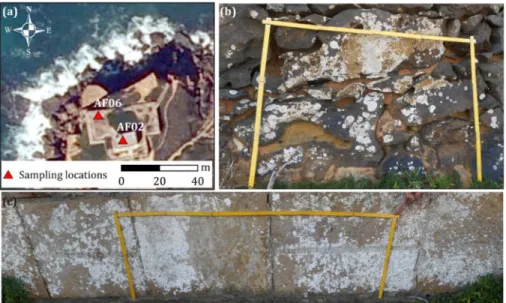
247 [insert Figure 5.]
248 Figure 5: (a), (b), (c) and (d) location of the boulder deposit and control points along the 249 coastline (Maps built with Esri© ArcMapTM 10.5.1.7333, source of satellite images: Esri,
250 DigitalGlobe, GeoEye, Earthstar Geographics, CNES/Airbus DS, USDA, USGS, AeroGRID,
251 IGN, and the GIS User Community)
252
253 Identification of lichen species 254 3 4 5 6 7 8 9 10 11 12 13 14 15 16 17 18 19 20 21 22 23 24 25 26 27 28 29 30 31 32 33 34 35 36 37 38 39 40 41 42 43 44 45 46 47 48 49 50 51 52 53 54 55 56 57 58
For Peer Review
255 Identification of voucher samples of lichens was based on macroscopical and microscopical 256 characters, and chemical features, following Clauzade and Roux (2002) and Smith et al. (2009). 257 In the field, lichen species was identified by scratching the areola and finding the color orange 258 due to the presence of carotenoids in the Trentepohlia photobiont (Friedl and Büdel, 2008). 259
260 Indirect measurements: Lichen size and cover 261
262 Three lichen age variables were tested: the average diameter of the largest inscribed circle 263 observed in the five largest thalli, as suggested by Innes (1985), hereafter named Ø (Figure 6a-b); 264 the area of the circle represented by Ø, herein represented as A, and obtained from the 265 mathematical expression relating the diameter and the area of a circle: 𝐴 = 𝜋
(
∅ 2)
2; and lichen 266 cover percentage over standard control-areas (Figure 6c-d). Control surfaces are steep (72° to 267 vertical), face North, and are near the coastline (<150m). The selection of the largest thalli was 268 based on visual inspection, and their measurement was performed to the closest millimeter using 269 a ruler. Measurements were made by the same operator to minimize errors associated with 270 between-operator variance (cf. Innes, 1985). Irregularities in growth rates due to coalescence were 271 avoided by sampling isolated thalli with clear margins and circular growth. Cover measurements 272 were performed in areas presenting the highest lichen cover. The sampling location was registered 273 using a Real-Time Kinematic Global Positioning System, and the azimuth and slope of each 274 surface was obtained with a compass and clinometer.275
276 [insert Figure 6.]
277 Figure 6: a) Opegrapha durieui thallus; (b) same extent as (a) showing the diameter of the 278 largest inscribed circle; (c) Mosaic of a surface colonized by Opegrapha durieui; (d) Same 279 extent as (c) after image processing and overlapping a 10mm10mm grid
280
281 Age determination of man-made control surfaces AF02- AF08, AF10, and AF11 were based on 282 the compilation of historical information of Portuguese monuments by Almeida (1946), Costa 283 (1997), Coutinho (1997), Mateus (1999), Mesquita (2000), Quaresma (2007), Machado (2009), 284 Silva (2013), Severino (2014), and by official government-issued bulletins describing the general 285 state and reconstruction of national monuments (Direção Geral dos Edifícios e Monumentos 286 Nacionais, 1953; 1960). For the man-made control surface AF01 and the rock-scar RF03, age 287 determination was based on the comparison of aerial photographs from 1980, 1989, and 2000. 288 For the rock-scars RF01 and RF02, age determination was based on field surveys and further 289 constricted by public photographic records of the area and by eye-witness accounts. In many 290 control points, it was only possible to attribute an age range, rather than a number. In these cases, 291 a middle date was assumed. Further details on age determination for all control surfaces are 292 available in SM.
293
294 Growth rates were determined by dividing the lichen age variable (diameter, area, or lichen cover) 295 with the age of the control surfaces. Local climatic variables (temperature, water vapor pressure, 296 solar radiation, and precipitation) with a resolution of ~1km, averaged for the years 1970-2000, 297 were extracted for each control point from the WorldClim Version2 climate dataset (Fick and 3 4 5 6 7 8 9 10 11 12 13 14 15 16 17 18 19 20 21 22 23 24 25 26 27 28 29 30 31 32 33 34 35 36 37 38 39 40 41 42 43 44 45 46 47 48 49 50 51 52 53 54 55 56 57 58 59
For Peer Review
298 Hijmans, 2017). Altitude, distance from the coastline, and average climatic variables were 299 compared with growth rates to assess the influence of environmental variables on lichen growth. 300 Although climatic changes associated with local factors cannot be assessed using a 1-km grid, it 301 allows us to assess climatic changes within control points related to coastline exposure (N versus 302 S-facing coastline) and along the W coast of Portugal.
303
304 The same lichen size sampling methodology was used in the control points and boulder deposit. 305 Opegrapha durieui was always found colonizing shaded surfaces, such as N-facing boulder faces, 306 faces shadowed by larger boulders, or undersides of tilted boulders. In four boulders, smaller 307 living lichen thalli were found persistently covering larger dead lichen thalli. In these cases, both 308 larger and smaller populations presented consistent sizes between them, indicating the generalized 309 death of the largest population. Given that lichens grew in the same boulder surface, lichen death 310 must have been caused by changes in environmental conditions (e.g., boulder burial by finer 311 sediments that washed out from sedimentary layers outcropping above, or temporary changes in 312 temperature/moisture) and not by boulder movement. Once optimal ecological conditions 313 resumed, so did lichen regrowth, here represented by the smaller population. In these cases, age 314 will be under-estimated and can only be attributed to the event that killed the largest population. 315 In the northern sector, cliffs located seaward of the boulder deposit were found colonized by the 316 lichen species. In this sector, and to avoid inheritance, only lichens colonizing undersides of 317 overturned boulders (surface initially facing upwards) were considered.
318
319 Quantification of lichen cover was based on photographs following the method of McCarthy and 320 Zaniewski (2001). A folding ruler was placed in front of the rock surface for scaling. Photographs 321 were taken with the camera parallel to the rock surface. Selected surfaces were photographed at 322 close range in small and partly overlapping sections to maintain the best resolution for mosaic 323 construction. Mosaics were built using photo stitching software (Adobe® Photoshop® or Hugin 324 version: 2013.0.0.0d404a7088e6) and scaled in geographical information system (GIS) software 325 (Esri® ArcMapTM). The lichen cover area was extracted using photo editing software (Adobe®
326 Photoshop®). Scaled mosaics containing the extracted areas were classified and converted into 327 polygons using automatic image classification tools from GIS software (Figure 6c). Areas clear 328 of lichen colonization were quantified and used to determine the percentage of lichen cover. The 329 polygons representing colonized surfaces were split into 100mm100mm grid cells (Figure 6d). 330 The grid cell showing the highest value of lichen cover was selected as an initial control surface 331 (minimum area considered). The surrounding grid cells were then successively summed in 332 100mm increments (200mm200mm, 300mm300mm, and so on), and the total area covered by 333 lichens was determined for each increment. Area covered, percentage and standard deviation were 334 plotted for each control point to determine the area better representing lichen age.
335
336 Lichen growth model 337
338 Assumptions of linear regression (normality of error distribution and homoscedasticity) were 339 verified in the dataset comprising % lichen cover, Ø, A, and age of control-surfaces. The error 340 distribution was tested for normality using a Shapiro-Wilk normality test, and the data were tested 341 for homoscedasticity using a t-score test for non-constant error variance (Fox and Weisberg, 3 4 5 6 7 8 9 10 11 12 13 14 15 16 17 18 19 20 21 22 23 24 25 26 27 28 29 30 31 32 33 34 35 36 37 38 39 40 41 42 43 44 45 46 47 48 49 50 51 52 53 54 55 56 57 58
For Peer Review
343 Team, 2017). In both tests, the p-values obtained were higher than 0.05, indicating that residuals 344 were normally distributed, and that the variance was constant. The growth model was based on 345 the best fit to lichen age variables vs. time using the lm function (stats package) in R software. 346 Moreover, age estimations were obtained with the function relating lichen size and age. Prediction 347 intervals, which provide an estimate of individual observations, were determined using the predict 348 function (stats package) also in R software, based on the following set of equations (Freund et al., 349 2006; Moore et al., 2009): 350 𝑝𝑟𝑒𝑑𝑖𝑐𝑡𝑖𝑜𝑛 𝑖𝑛𝑡𝑒𝑟𝑣𝑎𝑙𝑠 = 𝜇𝑦|𝑥± 𝑡∗𝑆𝐸𝑒𝑠𝑡𝑖𝑚𝑎𝑡𝑒 351 𝑆𝐸𝑒𝑠𝑡𝑖𝑚𝑎𝑡𝑒= 𝑀𝑆𝐸
(
1 +1 𝑛+(
𝑥∗ ― 𝑥)
2 𝑆𝑥𝑥)
352 𝑀𝑆𝐸 =Σ(𝑦 ― 𝜇𝑦|𝑥)
2 𝑛 ― 2 353 𝑆𝑥𝑥= Σ(𝑥 ― 𝑥)2354 Predicted values are denoted by 𝜇𝑦|𝑥, represents the critical point of the t distribution for the 𝑡∗ 355 desired significant level with (𝑛 ― 2) degrees of freedom, n being the number of observations. 356 Observed values of the dependent variable are represented by , 𝑦 𝑥∗ represents the specific value 357 of for which the intervals are determined and the mean of observed values of the independent 𝑥 𝑥 358 variable. Prediction intervals were determined considering a 0.95 confidence interval (2-sigma), 359 for which 𝑡(12) equals 2.179.
360
361 Direct measurements of lichen growth 362
363 Direct measurements were based on the comparison of photographic record taken on different 364 dates, inspired by the methodology described in Brabyn et al. (2005) and Roof and Werner (2010). 365 Photographs taken between 2013 and 2016 showed enough quality to differentiate and outline 366 thalli, and in some cases, to detect lichen coalescence. Surfaces included man-made and rock-scar 367 control surfaces north of the study area, namely AF02, AF03, AF05, AF06, RF01, and RF02 368 (Figure S6 in SM). These locations were revisited in January of 2020 to photograph isolated 369 lichens identified in the initial photographs. The 2020 photographs were georeferenced using 370 ESRI® ArcGIS™ version 10.4.0 based on an overlapping ruler. The older photograph was 371 overlapped to the more recent and georeferenced using at least ten features of the rock, such as 372 minerals and cracks, around the borders of each thallus (Brabyn et al., 2005; Roof and Werner, 373 2010). Image transformation due to georeferencing followed a polynomial equation that provided 374 a root mean square error (RMSE), used as an accuracy measure of the georeferencing process 375 (Brabyn et al., 2005). Lichen outlines were hand-traced over both photographs by the same 376 operator, thus creating polygons for each thallus (Roof and Werner, 2010). The maximum 377 inscribed circle for each polygon was automatically extracted using ET GeoWizards version 11.3 378 software, and the area was automatically determined in ArcGIS. The diameter of each circle was 379 computed from the area. When the sum of RMSE obtained from georeferencing was higher than 380 the difference between the diameters from different dates, the data were eliminated from further 381 analyses. 382 3 4 5 6 7 8 9 10 11 12 13 14 15 16 17 18 19 20 21 22 23 24 25 26 27 28 29 30 31 32 33 34 35 36 37 38 39 40 41 42 43 44 45 46 47 48 49 50 51 52 53 54 55 56 57 58 59
For Peer Review
383 Optically stimulated luminescence384
385 Two samples of the sand patch found beneath boulders were collected for age determination by 386 OSL (Figure 3b). Sample preparation was carried out under amber-light conditions. Samples were 387 wet sieved to extract the 90–150 m fraction, and then treated with HCl to remove carbonates 388 and with hydrogen peroxide to remove organics. Quartz and feldspar grains were extracted by 389 flotation using a 2.7 gm/cm3 sodium polytungstate solution, then treated for 60 minutes in 48%
390 HF, followed by 30 minutes in 47% HCl. The sample was then re-sieved, and the <90 m fraction 391 discarded to remove residual feldspar grains. The etched quartz grains were mounted on the 392 innermost 2 mm or 5 mm of 1 cm aluminum disks using Silkospray. Chemical analyses were 393 carried out using a high-resolution gamma spectrometer. Dose-rates were calculated using the 394 method of Aitken (1998) and Adamiec and Aitken (1998) and the updated dose-rate conversion 395 factors of Guerin et al. (2011). The cosmic contribution to the dose-rate was determined using the 396 techniques of Prescott and Hutton (1994).
397
398 OSL analyses were carried out on Riso Automated OSL Dating System Models TL/OSL-DA-399 15B/C and TL/OSL-DA-20, equipped with blue and infrared diodes, using the Single Aliquot 400 Regenerative Dose (SAR) technique (Murray and Wintle, 2000). Early background subtraction 401 was used (Ballarini et al., 2007; Cunningham and Wallinga, 2010). Preheat (240ºC/10 s) and 402 cutheat (220ºC/0 s) temperatures were based upon preheat plateau tests between 180º and 280ºC. 403 Dose-recovery was within 2-sigma of 100% and thermal transfer within 2-sigma of 0 Gy (Murray 404 and Wintle, 2003). Sample growth curves were below saturation (D/Do < 2; Wintle and Murray, 405 2006). Optical ages are based upon a minimum of 50 aliquots (Rodnight, 2008). Individual 406 aliquots were monitored for insufficient count-rate, poor quality fits (i.e., higher error in the 407 equivalent dose, De), poor recycling ratio, strong medium vs fast component (Durcan and Duller, 408 2011), and detectable feldspar. Aliquots deemed unacceptable based upon these criteria were 409 discarded from the data set before averaging.
410
411
Results
412
413 Lichen age variables (lichen cover, Ø and A) 414
415 Increments in the control area generated an increase in total area covered by lichens, accompanied 416 by a decrease in lichen cover percentage and by an increase in the standard deviation (Figure S19 417 in SM). In many cases, these changes were abrupt, rapidly stabilizing after the first 1-3 grid cell 418 increments. As the control area increased, a higher proportion of rock surface was added in 419 detriment of the area covered by lichens, due to measurements being centered in grid cells with 420 maximum lichen cover. Given that our objective was to find the region of the surface that was 421 primarily colonized, we focused on these first area increments (100mm100mm to 422 300mm300mm), where lichen cover was less diluted, and control surfaces showed a more 423 significant contrast. Also, area increments were limited by smaller control surfaces, such as the 424 cornerstone in the AF07 control point (Figure S13 in SM). The increase in control-area generates 3 4 5 6 7 8 9 10 11 12 13 14 15 16 17 18 19 20 21 22 23 24 25 26 27 28 29 30 31 32 33 34 35 36 37 38 39 40 41 42 43 44 45 46 47 48 49 50 51 52 53 54 55 56 57 58
For Peer Review
426 cover (Figure 7a) (detailed results in SM). To minimize the dilution, the 100mm100mm area 427 was considered as the most representative of surface age.
428
429 Opegrapha durieui reaches a cover of ~70% after 70 years of exposure (Table 1 and Figure 7a). 430 Abnormally high values were observed in two young sampling locations (67 and 157 years old), 431 indicating that this age variable is not strictly controlled by surface age. For example, control 432 surfaces AF02 and AF06 are in the same location with contrasting values in lichen cover (AF02 433 is lower in ~11% despite being 229 years older). We hypothesize that differences are related to 434 either rock slope (vertical in AF02 and 72° in AF06), rock-texture (AF02 is coarser), or surface 435 roughness (AF02 surface is more irregular) (Figures S24-26 and S29 in SM). These results 436 suggest that lichen cover is not a good age estimator, and this variable was excluded from further 437 analysis.
438
439 Table 1: Surface age, time since exposure, lichen cover, and size in the control surfaces. 440 441 Control Surface Surface age (calendar age) Time
(years) Lichen cover (%) Ø (mm) A (mm2)
RF01 2011-2012 1.7 0 0 0 RF02 2005-2006 7.6 3 5 20 AF01 1980-2000 23.9 2 13.2 137 RF03 1980-1989 29 6 11 95 AF02 1944-1949 67 94 24.4 468 AF10 1793 157 90 29.6 688 AF06 1657-1777 296 82 31.4 774 297 - 34.8 951 AF07 1657-1777 356 94 - -324 73 - -AF08 1588-1690 326 - 31.6 784 AF04 1678 338 95 33.0 855 AF03 1645 370 100 38.8 1182 382 71 - -AF09 1632 384 - 34.0 908 382 97 - -AF11 1632 384 - 37.2 1087 457 98 - -AF05 1558 458 - 37.6 1110 3 4 5 6 7 8 9 10 11 12 13 14 15 16 17 18 19 20 21 22 23 24 25 26 27 28 29 30 31 32 33 34 35 36 37 38 39 40 41 42 43 44 45 46 47 48 49 50 51 52 53 54 55 56 57 58 59
For Peer Review
443 Figure 7: Opegrapha durieui age variables plotted against time: (a) lichen cover considering 444 different control areas (b) Ø; and (c) A
445
446 Opegrapha durieui thalli become visible eight years after surface exposure. Lichen diameter, Ø, 447 increased at a linear rate of 0.36-0.66 mm/year (averaging 0.49 mm/year) up to ~70 years after 448 exposure. Growth rates based on Ø decreased pronouncedly afterward to 0.08-0.19 mm/year 449 (averaging 0.11 mm/year) (Table 1 and Figure 7b). Lichen diameter does not increase linearly 450 with time and is better described by a logarithmic function. Lichen area, A, shows a more steady 451 and constant increase with age, the growth rates averaging 3.18 mm2/year (Figure 7c). No
452 relationship was detected between lichen growth rates and ecological variables (altitude, distance 453 from the coastline, and climatic variables) (Figures S20-S21 in SM).
454
455 Growth models 456
457 Growth models for Ø and A, are represented in Figure 8a-b, showing an R2 of 0.96 and 0.91 (P<
458 0.0001), respectively, which indicates the high goodness of fit of both models. The high 459 correlation and the absence of a relationship with ecological variables suggest that the latter plays 460 a minor role in lichen growth and that Ø and A can be used as age estimators.
461
462 [insert Figure 8.]
463 Figure 8: (a) Ø and (b) A best fit and 95% prediction intervals. (c) Prediction bands for the Ø
464 and A models
465
466 R2 values obtained for the Ø-based model may suggest that it performs better and is the best age
467 estimator. Furthermore, prediction bands for lower Ø are much narrower than those for the A 468 model (Figure 8c). However, due to the exponential relationship between time and Ø, the 469 amplitude of prediction intervals becomes increasingly high for larger sizes, in cases doubling the 470 magnitude of predicted ages (Figure 8c). On the contrary, at ages of about 200 years and higher, 471 amplitudes of prediction intervals based on A remain around 235 years, while those based on Ø 472 continue to increase.
473
474 Direct measurement of lichen growth 475
476 Thalli monitored for lichen growth are shown in Figures S22 to S30 in SM (data in Appendix). 477 Manny lichens, especially the largest, were coalescing and were excluded to avoid competitive 478 restrictions in lichen growth. As a result, there is a higher frequency of measurements in smaller 479 thalli (<10mm). Only three thalli were measured in the oldest control point, AF05, all of them 480 missing apothecia and showing evidences of being affected by fungi, having also decreased in 481 size from 2016 to 2020. We believe that most thalli covering this surface are dead, possibly due 3 4 5 6 7 8 9 10 11 12 13 14 15 16 17 18 19 20 21 22 23 24 25 26 27 28 29 30 31 32 33 34 35 36 37 38 39 40 41 42 43 44 45 46 47 48 49 50 51 52 53 54 55 56 57 58
For Peer Review
483 lichens were already detected in 2013, but their frequency significantly increase since then. The 484 growth rates measured in the A05 control surface are not representative of active thalli and were 485 excluded from the dataset. Overall, 64 thalli were measured, from which 18 presented a 486 georeferencing RMSE higher than changes in lichen diameter, having also been excluded. This 487 exclusion affected all lichen sizes, but eliminated most of the largest monitored thalli, only one 488 remaining (Figure S31 in SM).
489
490 Growth rates show an increasing trend with thalli size for smaller lichen thalli (<10mm), ranging 491 from 0.03mm/year (0.10mm2/year) to 0.74mm/year (14.18mm2/year) (Figure 9a-b). The largest
492 thalli, measuring 26.12mm (535.95mm2), presented a meager growth rate of 0.09mm/year
493 (3.64mm2/year). The best fit function is a second-order polynomial, with an R2 of 0.71 for A and
494 of 0.19 for Ø. By removing the larger thallus, the best fit function becomes linear for both 495 variables (Ø and A), again more evident for A (Figure 9c).
496
497 [insert Figure 9.]
498 Figure 9: Growth rates plotted against lichen size. Direct growth rates and best fit 2nd
499 polynomial based on (a) Ø and (b) A. (b) Direct growth rates and best linear fit with the 500 exclusion of the largest thallus based on (c) Ø and (d) A. (e) Direct and inferred growth rates
501 based on (e) Ø and (f) A
502
503 The comparison of direct and inferred growth rates confirms the distinct behavior between smaller 504 and larger thalli (Figure 9e-f). Indirect growth rates of larger thalli (Ø>30mm or A>700mm2)
505 reach a constant value of ~0.09mm/year and ~4mm2/year for Ø and A, respectively. However,
506 indirect growth rates of younger thalli are slightly lower than for direct measurements, especially 507 for A. Further validation of the growth models was based on the identification of lichens in an 508 originally uncolonized rock-fall surface (RF01: 2011-2012) (Figure S22 in SM) indicating an 509 establishment period under eight years, contained within prediction intervals of both Ø and A 510 model
511
512 Age estimation of the boulder deposit 513
514 OSL age estimation of the marine sand fond beneath boulders is presented in Table 2. 515 Determination of average De values was carried out using the Minimum Age Model (Galbraith 516 et al., 1999) because the De distribution (asymmetric distribution; decision table of Bailey and 517 Arnold, 2006), indicated that it was more appropriate than the Central Age Model (Galbraith et 518 al., 1999). Results for both the Minimum and Central Age Models are further presented in SM. 519 Samples have an estimated age of 23020 and 290 50 years, the marine sand having been 520 deposited between 1674 and 1804.
521
522 Table 2: OSL dating results when applying the Minimum Age Model (Galbraith et al., 1999) 523 (OSL ages in years before 2014). Error on De is 1 standard error. Age error includes random 3 4 5 6 7 8 9 10 11 12 13 14 15 16 17 18 19 20 21 22 23 24 25 26 27 28 29 30 31 32 33 34 35 36 37 38 39 40 41 42 43 44 45 46 47 48 49 50 51 52 53 54 55 56 57 58 59
For Peer Review
Sample ID Lab ID Burial depth (m) Dose Rate (Gy/ka) De (Gy) Number of aliquotsAge (a) Cal. Age (CE-Current Era) Q20CxS UNL4003 0.35 2.660.10 0.600.06 75 23020 1784 Q21CxS UNL4004 0.35 2.630.10 0.770.13 72 29050 1724 525
526 Information regarding boulder mass, lichen parameters, and estimated ages using the lichen 527 growth models are shown in Table S3 (SM) and depicted in Figure 10. Extrapolated ages of older 528 boulder stabilization are quite different between models, reaching 25 BCE (Before current era) 529 (3165 BCE-1211 CE) with the Ø-based model and 1348 CE (1201-1494 CE) with the A-based 530 model. However, interpolated ages roughly overlap between models, the significant difference 531 being the amplitude of prediction intervals. Results from both models indicate that only 6-9 532 boulders were stabilized before 1755 (19% with the Ø-based model to 28% with the A-based 533 model) and even less overlap the 1755 tsunami (12% versus 19%). These include the largest 534 boulders colonized by lichens in the study area, forming a boulder cluster located in the northern 535 sector of the study area (Figure S3a in SM). Results obtained with both models show that most 536 boulders have only recently stabilized, and their final movement cannot be attributed to the 1755 537 Lisbon tsunami. Furthermore, boulders that have been emplaced far back in time are generally 538 larger than those recently stabilized.
539
540 [insert Figure 10.]
541 Figure 10: Estimated ages plotted against boulder mass. Lighter dots representboulders with 542 two overlapping populations. Horizontal error bars represent 95% prediction intervals. The grey 543 line corresponds to 1755 (date of the Lisbon tsunami). The dashed grey line represents the
544 interpolation limit
545 546
547
Discussion
548
549 Lichen growth model 550
551 Preliminary results of lichen cover showed abnormally high values in two young control surfaces 552 (67 and 157 years), contrasting with similar or even lower cover obtained for older surfaces (>290 553 years). Thus, lichen cover as shown to be dependent on other variables apart from time. The 554 comparison of ecological variables from a 67-year old fort (AF02) (94% lichen cover) with an 555 older nearby control surface of 296 years (AF06) (82% lichen cover) revealed differences in 556 surface slope, rock texture, and surface roughness. We hypothesize that Opegrapha durieui favors 557 colonization in coarse-grained limestone rocks forming vertical and rough surfaces. A higher 558 affinity to steeper slopes has been reported for lichen species that preferably colonize north-facing 559 rock surfaces (Armstrong, 1974a). Furthermore, higher surface roughness provides a higher 3 4 5 6 7 8 9 10 11 12 13 14 15 16 17 18 19 20 21 22 23 24 25 26 27 28 29 30 31 32 33 34 35 36 37 38 39 40 41 42 43 44 45 46 47 48 49 50 51 52 53 54 55 56 57 58
For Peer Review
561 smoother surface (Armstrong, 1974a). Finally, rocks with coarser textures also retain more 562 moisture than fine-textured rocks (Benedict, 1967). Altogether, the rock-type available for 563 colonization in AF02 offers a broader spectrum of microhabitats and higher water retention 564 capability, which could explain differences in the rate of lichen colonization and, consequently, 565 lichen cover percentages. Similar results have been obtained in other regions and with different 566 species, leading to the conclusion that lichen cover is more sensitive to environmental variations 567 than lichen size (Innes, 1986; McCarthy and Zaniewski, 2001).
568
569 The logarithmic correlation between Ø and time is in line with results described worldwide by 570 Bradwell (2001), Gob et al. (2003), Benedict (2009), and Armstrong (2015), among others. The 571 logarithmic correlation is attributed to changes in growth rate and is interpreted by Armstrong 572 (1974b) as distinct stages in lichen development. However, the contrast in growth rate between 573 smaller and larger thalli is less apparent when indirectly measured A is considered (red data series 574 in Figure 9f). The discrepancy of changes in growth rate within lichen age variables partly results 575 from the quadratic relationship between A and Ø (further explained in SM). This geometrical 576 relationship generates an inflated decrease in lichen growth as it becomes larger/older, further 577 increasing the contrast between growth rates obtained with both age variables.
578
579 The choice of the variable that better represents lichen growth must be based on biology. In this 580 regard, increases in the size of crustose lichens occur along an area due to marginal growth and 581 in thickness, volume, or mass (cf. Armstrong, 1974b; Hill, 1981; Máguas and Brugnoli, 1996; 582 Clark et al., 2000; Seminara et al., 2018). So in what concerns growth in two dimensions, the area 583 is a more realistic representation of lichen growth when compared to diameter. In fact, area 584 measurements have been considered has more precise than single-axis measurements, as they 585 include growth around the entire perimeter of the thallus (Roof and Werner, 2011). Different radii 586 contribute to growth at different times, especially when thalli are not perfectly circular (Matthews 587 and Trenbirth, 2011). Consequently, irregular, but significant changes occurring along the 588 perimeter of a thallus are not incorporated in lichen growth measurements when changes in 589 diameter are considered (Roof and Werner, 2011).
590
591 Our observations show that lichen growth-rates change with lichen size, linearly increasing up to 592 a point, and then decreasing until reaching a constant value. However, evidence of decreasing 593 growth rates based on our dataset of direct measurements are weak, involving only one thallus, 594 the relationship being perfectly linear if the larger thallus is excluded (Figure 9c-d). Similar 595 observations were reported by Roof and Werner (2011) and attributed to the scarcity of isolated 596 larger thalli and consequent poor constrain of growth rates. Regardless, the polynomial behavior 597 of directly measured lichen growth against size has been reported in several works on crustose 598 lichens (e.g., Bradwell and Armstrong, 2007; Matthews and Trenbirth, 2011). These changes in 599 growth rate are attributed to different phases of growth in the juvenile phase (increasing growth 600 rates), maturation (constant high growth rates), and maturity/senescence (declining to constant 601 low growth rates) (Armstrong, 1974a; Bradwell and Armstrong, 2007).
602
603 The linear increase in the size of smaller thalli is more evident for directly measured lichen growth 604 (increase in factor of 150) than for interpolated lichen growth (increase in factor of 3) (Figure 9f). 605 The mismatch between direct and indirect-derived lichen growth rates has been a highly debated 606 issue and attributed to population dynamics. According to Loso and Doak (2006), older lichens 3 4 5 6 7 8 9 10 11 12 13 14 15 16 17 18 19 20 21 22 23 24 25 26 27 28 29 30 31 32 33 34 35 36 37 38 39 40 41 42 43 44 45 46 47 48 49 50 51 52 53 54 55 56 57 58 59
For Peer Review
607 are progressively harder to find on older surfaces, the probability of finding original cohorts 608 decreasing in time. In agreement, interpolated growth rates based on lichen size on a surface of 609 known age would be under-estimated. Lichen death was frequently observed in control surfaces 610 when comparing photographs 3-6 years apart, attesting a high lichen turnover. Another factor 611 contributing to lower values for the indirectly measured dataset is that it results from averaging 612 five individuals, which inevitably leads to underestimated growth rates. However, this method 613 equally affects control and boulder surfaces, so age estimations based on the models are not 614 compromised.
615
616 Age estimation of the boulder deposit 617
618 The marine sand found beneath the boulders comprises fine, well-sorted sand, mostly consisting 619 of quartz grains. The Coxos beach sand and sand deposited during storms in the rocky platform 620 comprises moderately to well-sorted coarse sand with bioclasts, and the colluvium consists of 621 very poorly sorted medium sand with lithoclasts (Oliveira, 2017). The composition, textural, and 622 morphoscopic characteristics of the sand patch contrast with present-day sediments. Furthermore, 623 grain size characteristics of the sand patch are compatible with sediments found in the nearshore, 624 mostly comprising patches of moderately sorted and negatively skewed sand within rocky 625 outcrops (cf. Balsinha, 2008). We hypothesize that the sand fraction from the sand patch was 626 sourced offshore the closure depth of storms reaching the study area. Ultimately, present-day 627 transport inland and deposition of sediments located offshore the closure depth could be 628 associated with a tsunami inundation. Since OSL ages perfectly overlap the 1755 Lisbon tsunami 629 and historical records indicate that this event reached a minimum inundation height of 5m in this 630 region (cf. Oliveira, 2017), the marine sands may be tsunami-related. The asymmetric shape of 631 the dose distributions in OSL age estimation of onshore sand deposits is frequently interpreted as 632 insufficient light exposure for complete bleaching during the rapid transport and deposition during 633 these events (e.g., Cunha et al., 2010; Sawakuchi et al., 2012; Fruergaard et al., 2013). Although 634 this occurs for both storm and tsunami-related deposits, for the former, they are described in 635 progradational shorelines, in which the amount of sediment available for transport facilitates 636 incomplete bleaching (Sawakuchi et al., 2012; Fruergaard et al., 2013). This is not the case for 637 the sand-starved rocky shoreline under analysis. It is more likely that the sand patch was deposited 638 by the 1755 tsunami, which raises the possibility that this inundation has reached the study area. 639 Consequently, the deposition of the boulders over the sand patch must be either coeval or 640 subsequent to the 1755 tsunami.
641
642 Age estimation using lichenometry provides a minimum age of boulder emplacement and/or 643 reworking. The distinction between both cases can only be tentatively made when there is 644 evidence of lichen death and regrowth (e.g., the existence of overlapping distinct populations). 645 Over 72% of dated boulders have reached a stable position long after the 1755 tsunami. No other 646 tsunami reaching the western Portuguese coastline in the past 1000 years could generate the 647 movement of supratidal boulders (cf. Andrade et al., 2016). There is no guarantee that 91% of 648 these rock boulders (9% were emplaced before 1755) were not placed in the rocky platform by 649 the 1755 tsunami inundation and have been moving since then due to inundations related with 650 storm events. However, the remaining 9% must have been transported by storms.
651 3 4 5 6 7 8 9 10 11 12 13 14 15 16 17 18 19 20 21 22 23 24 25 26 27 28 29 30 31 32 33 34 35 36 37 38 39 40 41 42 43 44 45 46 47 48 49 50 51 52 53 54 55 56 57 58
For Peer Review
652 Furthermore, boulder detachment from the edges of the platforms occurred along the study area 653 during the storms of 2013/2014. In several locations, boulders up to 13t could be traced back to 654 their original location in the platform and cliff edges (Oliveira, 2017). These observations are 655 meager when compared to the maximum boulder size of 620t moved by the same storms in Ireland 656 (Cox et al., 2018). Boulder dislodgement from the edge of cliffs and rocky platforms is facilitated 657 by the presence of embayments and overhanging configurations of impacted cliffs (Canelas et al., 658 2014). The joint-bounded protruding limestone layers in the upper geological units, together with 659 the natural indentations in the lower rocky platform, provide the optimal morphological 660 conditions for boulder detachment and emplacement over the structural surface. This 661 interpretation agrees with the spatial pattern in boulder size observed in the study area, showing 662 larger boulders preferably located inland of indentations.
663
664 The dynamic character of this coastline probably contributes to the low number of colonized 665 boulders in this deposit. Colonization of boulders by Opegrapha durieui was mostly found in the 666 middle of more developed and stable boulder ridges. Closer to the platform edge, the absence of 667 Opegrapha durieui could be associated with the frequency in boulder movement together with 668 the direct and frequent effect of sea spray, where other lichen species grow. Closer to the inner 669 edge of the platform, stabilization is compromised by the cover of sediments from the colluvium 670 transported by gravity and surface run-off.
671
672 Ultimately, boulder movement by storms in this rocky coastline must have been persistent since 673 at least 6000 calendar years BP, after the sea level stabilized close to its present position (Cearreta 674 et al., 2007). Larger boulder size, together with the higher elevation and distance from the 675 coastline, makes removal by lower-energy waves less probable, the largest/least accessible 676 boulders remaining immobile over the structural platforms. In agreement, the existence of only a 677 few boulders older/coeval to 1755, which are also generally larger, strongly suggests that erosion 678 has played an essential role in this location. Given the presence of both tsunami and storm events, 679 the movement of rock particles can be associated with both events been reshaping this coast since 680 sea-level stabilization. However, the high frequency in recent boulder stabilization strongly 681 suggests a storm origin for most of the deposit. The highest energy events, which include storms 682 and tsunamis, bear the potential to emplace the largest boulders (>10t). All other smaller rock 683 particles having been entrained and deposited by more common storm waves, only to be later 684 moved by subsequent events, remaining unaltered over the structural platforms during a residence 685 period rarely exceeding 200 years. An alternative explanation to the scarcity of boulders older 686 than the 1755 event, is that the tsunami inundation imparted an erosive signature in this location 687 and that boulders previously placed by storms were removed by the tsunami continuous and 688 persistent flow over the structural platforms.
689
690 The location and complex organization of boulder accumulation described herein show striking 691 similarities with known storm boulder deposits along the rocky western coast of Europe (e.g., 692 Etienne and Paris, 2010; Hall et al., 2006; Hansom and Hall, 2009; Cox et al., 2012). Similarities 693 include the organization of the boulders in ridges and clusters with imbricated boulders, location 694 on top of rocky cliffs, and size-grading inland. In contrast, boulder deposits related to 695 contemporary tsunamis mostly comprise boulder fields showing no organization or grading inland 696 (Etienne et al., 2011). These similarities further support the storm origin hypothesis and contrast 697 with the attribution of other boulder deposits in Portugal to palaeotsunamis, solely based on their 698 size (10-20t) and height above the reach of storm waves (~12m amsl) (Scheffers and Kelletat, 3 4 5 6 7 8 9 10 11 12 13 14 15 16 17 18 19 20 21 22 23 24 25 26 27 28 29 30 31 32 33 34 35 36 37 38 39 40 41 42 43 44 45 46 47 48 49 50 51 52 53 54 55 56 57 58 59
For Peer Review
699 2005). The re-assessment of these and other deposits could have important implications in risk 700 assessment and for coastal management.
701 702
703
Conclusions
704
705 By using control points with similar climatic variables, near-vertical surfaces facing North, 706 isolated thalli, measurements by a single operator, and by avoiding inheritance, we have 707 successfully constructed a lichen growth model validated by direct measurements. The model 708 provides a measure of uncertainty that incorporates fluctuations in growth rates resulting from 709 several possible factors, such as uncertainties in age determinations, environmental changes, and 710 the period of lichen colonization. Wide prediction intervals are related to the low number of 711 control points. However, given that our main objective was to estimate the age of boulder 712 stabilization to clarify the origin of the Coxos boulder deposit (tsunami vs. storm), uncertainties 713 of ~235 years for the A-based model are sufficiently low to provide an answer.
714
715 The model allowed estimating the age of exposure, including uncertainty intervals, of carbonate-716 based rocks, near the coastline, where other techniques could not be applied. Ultimately, it 717 demonstrates that many problems associated with lichenometry mentioned in the bibliography 718 arise from misuses of the technique, rather than lack of scientific grounds for its use. It further 719 demonstrates that many source errors associated with lichenometry can be minimized with 720 adequate sampling designs. Finally, the proposed model retains the well-appreciated 721 characteristics associated with lichenometry, such as simplicity, cost-effective, quick to apply, 722 and non-destructive.
723
724 Transference of this model to other locations in not advised without model validation with local 725 measurements, preferably based on indirect measurements, as they incorporate regional 726 ecological changes, e.g., temperature, precipitation, and pollution. An additional limitation to the 727 use of indirect lichen growth curves is that they represent the size of lichens before measurement 728 and, if applied to later studies, will not include changes in the interim period (Innes, 1985). 729 Furthermore, the application of this model is limited to limestone surfaces that have been exposed 730 in the past 500 years.
731
732 We demonstrate that the significant decrease observed in lichen growth rates based on diameter 733 is, in part, an inheritance of the quadratic relationship between the diameter of a circle and its 734 area. Changes in growth rates based on lichen diameter described by several authors and attributed 735 to different growth stages are only slightly observed in the indirect dataset based on the area of 736 the thalli. The area presents a linear relationship with time and changes attributed to senescence, 737 and competitive restrictions are not detected using this parameter. This suggests that the use of 738 Opegrapha durieui in lichenometric studies can be further extended in time, given that additional 739 and older control points are added to the model.
740 3 4 5 6 7 8 9 10 11 12 13 14 15 16 17 18 19 20 21 22 23 24 25 26 27 28 29 30 31 32 33 34 35 36 37 38 39 40 41 42 43 44 45 46 47 48 49 50 51 52 53 54 55 56 57 58
For Peer Review
741 The high frequency in boulder stabilization at the study site strongly suggests a storm origin for 742 this accumulation. These results show that storms can generate these deposits and challenge the 743 interpretation that they were formed during tsunamis. Consequently, the frequency of tsunami 744 events inferred from boulder deposits in the W coast of Portugal, and elsewhere, may be lower 745 than expected. The findings reported in this work agree with recent studies showing that storms 746 reaching the W coast of Europe generate frequent and significant boulder transport. Finally, the 747 presence of marine sand with ages compatible with the 1755 tsunami inundation, strongly 748 suggests that this event has reached this location at the height of 9m amsl (4m higher than the 749 assumed value for this region). Finally, the scarcity of boulders older than 1755 could indicate an 750 erosive signature for tsunamis in rocky coastline contexts.
751
752
References
753 Adamiec G and Aitken M (1998) Dose-rate conversion factors: update. Ancient TL, 16 (2): 37-754 50.
755 Aitken MJ (1998) An introduction to Optical Dating - The Dating of Quaternary Sediments by 756 the use of photon-stimulated Luminescence. New York. Oxford University Press.
757 Almeida J (1946) Roteiro dos monumentos militares portugueses, Vol II Distritos de Aveiro, 758 Coimbra, Leiria e Santarém. Almeida J (in Portuguese).
759 Andrade C, Freitas MC, Oliveira MA and Costa PJM. (2016) On the sedimentological and 760 historical evidences of seismic-triggered tsunamis in the Algarve coast of Portugal. In: Duarte J 761 and Schellart W (eds) Plate Boundaries and Natural Hazards - Geophysical Monograph 219, New 762 Jersey, American Geophysical Union and John Wiley and Sons, Inc, pp. 219-238.
763 Aptroot A and van Herk CM (2007) Further evidence of the effect of global warming on 764 lichens, particularly those with Trentepohlia phycobionts. Environmental Pollution, 146: 293-765 298.
766 Armstrong AR (1974a) The Descriptive Ecology of Saxicolous Lichens in an Area of South 767 Merionethshire, Wales. Journal of Ecology, 62(1): 33-45.
768 Armstrong RA (1974b) Growth phases in the life of a lichen thallus. New Phytologist, 73: 913-769 918.
770 Armstrong RA (2004) Lichens, lichenometry and global warming. Microbiologist, 5: 32-35. 771 Armstrong RA (2015) The influence of environmental factors on the growth of lichens in the 772 field. In: Upreti DK, Divakar PK, Shukla V and Bajpai R (eds) Recent Advances in Lichenology. 773 Springer, pp.1-18.
774 Armstrong RA (2016) Lichenometric dating (lichenometry) and the biology of the lichen genus 775 Rhizocarpon: Challenges and future directions. Geografiska Annaler: Seria A, Physical 776 Geography, 98(3): 183-206.
777 Bailey RM and Arnold LJ (2006) Statistical modeling of single grain quartz De distributions and 778 an assessment of procedures for estimating burial dose. Quaternary Science Reviews, 25: 2475-779 2502.
780 Ballarini M, Wallinga J, Wintle AG and Bos AJJ (2007) A modified SAR protocol for optical 781 dating of individual grains from young quartz samples. Radiation Measurements, 42(3): 360-369. 3 4 5 6 7 8 9 10 11 12 13 14 15 16 17 18 19 20 21 22 23 24 25 26 27 28 29 30 31 32 33 34 35 36 37 38 39 40 41 42 43 44 45 46 47 48 49 50 51 52 53 54 55 56 57 58 59