Buffer allocation in general single-server queueing networks

www.elsevier.com/locate/cor

Buffer allocation in general single-server queueing networks

F.R.B. Cruz

_{, A.R. Duarte}

_{, T. van Woensel}

a_{Department of Statistics, Federal University of Minas Gerais, 31270-901 Belo Horizonte, MG, Brazil}

b_{Department of Operations, Planning Accounting and Control, Eindhoven University of Technology, Eindhoven, The Netherlands}

Available online 12 March 2007

Abstract

The optimal buffer allocation in queueing network systems is a difficult stochastic, non-linear, integer mathematical programming problem. Moreover, the objective function, the constraints or both are usually not available in closed form, making the problem even harder. A good approximation for the performance measures is thus essential for a successful buffer allocation algorithm. A recently published two-moment approximation formula to obtain the optimal buffer allocation in general service time single queues is examined in detail, based on which a new algorithm is proposed for the buffer allocation in single-server general service time queueing networks. Computational results and simulation results are shown to evaluate the efficacy of the approach in generating optimal buffer allocation patterns.

䉷_{2007 Elsevier Ltd. All rights reserved.}

Keywords:Buffer allocation; Queues; Networks

1. Introduction

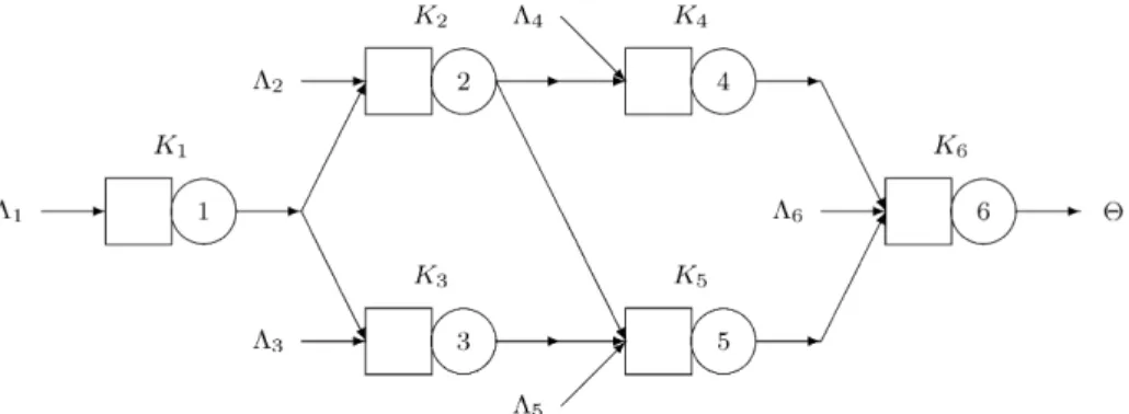
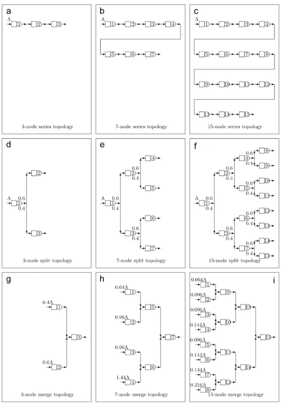
Manufacturing, telecommunication, and material handling systems are just few examples of practical interest that may be represented by finite buffer queueing networks. Because of the critical costs for buffer space, it is crucial to optimally determine the buffer spaces in order to ensure maximum performance at the lowest possible cost. The buffer allocation problem (BAP) is computationally hard to solve as the BAP is usually formulated as a stochastic, non-linear, integer mathematical programming problem. The BAP is to find optimal values for the buffer sizesKsuch that the blocking probabilitypKis below some pre-specified thresholdεfor all queues in the network. In this article, the BAP will focus on networks ofM/G/1/K queues, which in Kendall’s notation considers Markovian arrivals, generally distributed service times, one single server, and the total capacity ofKitems, including the item in service. In this case, the BAP is a complicated problem as it involves general service time queues configured in arbitrary networks[1]as seen inFig. 1. No closed-form objective functions are available for these types of networks. Thus, one needs to rely on approximations.

One of the objectives of this article is to extensively compare approximations for the blocking probability,pK, the probability that an arriving entity finds the queueing system at its capacity, in general single-server queues. One of the most regarded performance measures of queueing systems, the blocking probability is a building block for buffer allocation formulations. Another objective is to assess the accuracy of a novel implementation[2]for the generalized

∗Corresponding author. Tel.: +55 31 3499 5929; fax: +55 31 3499 5924.

E-mail addresses:fcruz@ufmg.br,fcruz@est.ufmg.br(F.R.B. Cruz),andersonrd@ufmg.br(A.R. Duarte),T.v.Woensel@tm.tue.nl (T. van Woensel).

Fig. 1. Queueing network in an arbitrary topology.

expansion method (GEM), a well-known method for performance evaluation of finite queueing networks, applied to networks ofM/G/1/Kqueues. Finally, the third objective is to propose a simple algorithm for the BAP in arbitrarily configured, finite buffer, single-server queueing networks. This will then result in insights into this challenging network design problem.

This article is organized as follows. In Section 2, the BAP is defined as a non-linear mathematical programming formulation and a short literature review is presented on the different algorithms developed in the past for similar problems. Some of the most effective approximations forpK are extensively compared in Section 3. In Section 4, the performance evaluation algorithm for finite queueing networks is described and its accuracy is tested. Then, Section 5 describes the proposed algorithm to solve the BAP. Computational results evaluating the efficacy of the new buffer allocation algorithm are discussed in Section 6. Finally, Section 7 closes the article with final comments and topics for future research in the area.

2. Buffer allocation problem

2.1. Problem formulation

The BAP is concerned with how much space needs to be allocated in order to guarantee that the probability of loosing clients (or delaying them) is below a certain threshold. In its simplest definition the BAP seeks the lowest integerK >0 such thatpKεfor some acceptable thresholdε∈(0,1). It is assumed that the system utilization(that is, the ratio between the arrival rate and the service rate,₌/) is below 1.0, because an optimum may not exist forKif1.0 (see Kimura[3]).

The BAP may be defined by a multi-objective non-linear mathematical programming formulation with integer decision variables xi ≡ K, for the ith M/G/1/K queue. However, in this article the following single objective formulation will be considered:

Z₌min i

xi (1)

s.t.

(x)min, (2)

xi ∈N, ∀i, (3)

2.2. Literature overview

The BAP literature can roughly be divided into four methodological approaches: simulation methods, metaheuristics, dynamic programming, and search methods. In the following paragraphs, a short overview of these approaches will be presented.

Thesimulationmethods aim to represent the actual systems by means of robust assumptions. In other words, general probability distributions are used to model the various aspects of the system, such as inter-arrival times, batch size of the arrivals, service times, among others. Simulation methods are usually very general and efficient but the price paid is a great computational effort that may reduce the size of treatable instances. However, successful uses of simulation methods have been reported by researchers, such as, for instance, Soyster et al.[4], for series queueing networks, and Baker et al.[5], for general topologies.

Metaheuristicsare very popular methods nowadays, mainly because of the increasing computational capacity avail-able. Typical techniques that fall into this area include simulated annealing, tabu search, and more recently, generic algorithms. The advantages of metaheuristics are the absence of all those restrictive assumptions usually required by the traditional methods and the ability of avoiding local optima traps in the seek of the global optimum. The disadvantage is that usually the metaheuristics must be tailored to the special structure of the problem. Among others, a successful case of use was reported by Spinellis et al.[6], for buffer allocation in tandem networks ofM/M/c/Kqueues.

Dynamic programmingis another powerful and reasonable approach for the BAP. Usually the exponential space complexity of dynamic programming methods reduces their applicability to very small size instances. However, the approach has been proved successful in many cases. For instance, Kubat and Sumita[7]and Yamashita and Altiok[8] reported results for networks ofM/M/1 queues in series and Yamashita and Onvural[9], for general topologies.

Finally, there are thesearch methods, which try to solve the problems avoiding the combinatorial explosion of possible solutions by choosing those solutions that are close to the optimum results. Their main disadvantage is their restrictive assumptions, such as concavity and convexity, that may limit the applicability. In the past, search methods were also successful in solving the BAP. In series topologies, the BAP was solved by search methods by Altiok and Stidham[10], for networks ofM/M/1/K queues, and by Hillier and So [11], forM/Ek/1/K queues. In general topologies, for instance, there are results reported by MacGregor Smith and Chikhale[12]and MacGregor Smith and Daskalaki[13], forM/M/1/Kqueues.

For networks of single-server general service time queues configured in general topologies, which is the main object of this article, there are not many results besides those reported by MacGregor Smith and Cruz[1]with a methodology based on Powell’s algorithm. The algorithm proposed in this article also falls into this category of search methods but is considerably simpler and easier to implement, compared e.g. to MacGregor Smith and Cruz[1].

3. Blocking probability

Accurate approximations for the blocking probability forM/G/1/Ksystems,pK, will be presented in the following paragraphs. They are based on finite Markovian systems,M/M/1/K, but approximations based on infinite queueing systems are also common. The relevance of accurate approximations for the BAP is apparent when we take into account that the throughput in a single queue is the following function of the arrival rate and the blocking probability:

=(1−pK).

3.1. Markovian systems

The blocking probability expression for a finite Markovian system is well known[14]

pK=

(1₋)K

1₋K+1 (4)

for = 1, being possible then to expressKin terms of, the system utilization, andpK, the blocking probability, as follows:

K₌

ln(pk/(1−+pk)) ln()

in which_⌈x_⌉is the lowest integer not inferior tox, and the blocking probability may be expressed in terms of the threshold throughput,min, and the arrival rate,, as

pK1− min

.

Expression (5) is not only useful for the optimal buffer allocation for individual Markovian queues but it is also useful for networks of general service time queueing systems, as shortly it will be apparent.

3.2. Gelenbe’s approximation

Generally speaking, approximations developed in the past for the blocking probability are based on infinite queues. Actually, many of them could be adapted forM/G/1/Kqueues. A survey by Makens[15], for instance, analyzed five different approximations and concluded that Gelenbe’s formula[16]was efficient for the majority of the cases tested. Gelenbe’s approximation is based on an approximation of the discrete queueing process by a continuous diffusion process. The blocking probability is given by

pk=

(₋)e−2((−)(k−1))/(c2a+c2s)

(2₋2_e−2((−)(k−1))/(c2 a+c2s)₎

, (6)

in whichis the arrival rate,, the service rate,c_a2₌Var(Ta)/E(Ta)2 is the squared coefficient of variation of the inter-arrival time, Ta, andcs2=Var(Ts)/E(Ts)2 is the squared coefficient of variation of the service time,Ts. From Eq. (6), it is possible to explicitly get the optimal buffer allocation

K₌2−2+ln((pK 2_)/((

−₊₊pK)))c2_a+ln((pK2)/((₋₊₊pK)))c_s2

2(₋) . (7)

Taking both the squared coefficients of variation of the inter-arrival time and the service time equal to 1,c_a2₌c2_s=1, Eq. (7) results in the optimal buffer allocation of Markovian single queues,M/M/1/K. Notice that the resulting expression will not be exactly theM/M/1/K formula, Eq. (5), because Gelenbe’s expression is an approximation. However, as noticed by Makens[15]and by MacGregor Smith and Cruz [1], Gelenbe’s expression is accurate for Markovian system, while is not accurate for deterministic service time systems,M/D/1/K.

3.3. Two-moment approximation

The two-moment approximation scheme is based on a weighted combination of some approximation for the optimal buffer expressions for Markovian systems,M/M/1/K, denoted byKM, and for deterministic service time systems,

M/D/1/K, denoted byKD. Tijms’ formula[17]is one two-moment approximation that has been shown to be very good in practice. It is given by

KTijms(c2s)=c2sKM+(1−c2s)KD (8)

forc_s20. Clearly, Tijms’ formula is exact for the extreme cases, i.e.,c2_s=0 andc2_s=1, if exact expressions are known forKMandKD.

Kimura’s formula[18]is another good two-moment approximation, which is a little simpler as it uses as a basis only an approximation for the optimal pure buffer expression of Markovian systems

BKimura(c2_s)₌BM₊NINT

(c_s2₋1) 2

√

BM

, (9)

rho

pK

0.0 0.5 1.0 1.5 2.0

s^2=1.0; K=2

rho

pK

0.0 0.5 1.0 1.5 2.0

s^2=1.0; K=4

rho

pK

0.0 0.5 1.0 1.5 2.0

s^2=1.0; K=8

rho

pK

0.0 0.5 1.0 1.5 2.0

s^2=1.0; K=16 0.6 0.5 0.4 0.3 0.2 0.1 0.0 0.6 0.5 0.4 0.3 0.2 0.1 0.0 0.6 0.5 0.4 0.3 0.2 0.1 0.0 0.6 0.5 0.4 0.3 0.2 0.1 0.0

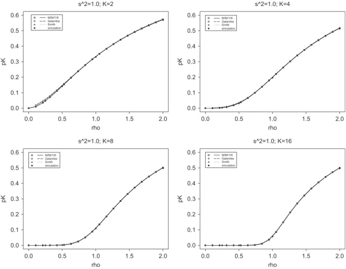
Fig. 2. Comparisons forpKfor Markovian systems.

Recently, MacGregor Smith[19]proposed the following two-moment approximation forM/G/1/Kqueues, based on Kimura’s formula

BSmith(c2_s)₌ ⎡ ⎢ ⎢ ⎢ ⎢ ⎣

ln(pK/(1−+pK))

ln() −1

BM

=KM−1

⎤ ⎥ ⎥ ⎥ ⎥ ⎦ +(c 2 s −1)

2 √ ⎡ ⎢ ⎢ ⎢ ⎢ ⎣

ln(pK/(1−+pK))

ln() −1

BM

=KM−1

⎤ ⎥ ⎥ ⎥ ⎥ ⎦ , (10)

in which expression (5), subtracted by the space for the single server, is used as the estimate for the optimal pure buffer allocation of Markovian systems,BM. Now, factoring the terms of the approximation, the following simplified expression for the optimal buffer size inM/G/1/Kis given:

BSmith(c2_s)₌[ln(pK/(1−+pK))−ln()](2+

√_c2 s −√)

2 ln() . (11)

rho

pK

0.0 0.5 1.0 1.5 2.0

s^2=0.5; K=2

rho

pK

0.0 0.5 1.0 1.5 2.0

s^2=0.5; K=4

rho

pK

0.0 0.5 1.0 1.5 2.0

s^2=0.5; K=8

rho

pK

0.0 0.5 1.0 1.5 2.0

s^2=0.5; K=16 0.6

0.5

0.4

0.3

0.2

0.1

0.0

0.6

0.5

0.4

0.3

0.2

0.1

0.0

0.6

0.5

0.4

0.3

0.2

0.1

0.0

0.6

0.5

0.4

0.3

0.2

0.1

0.0

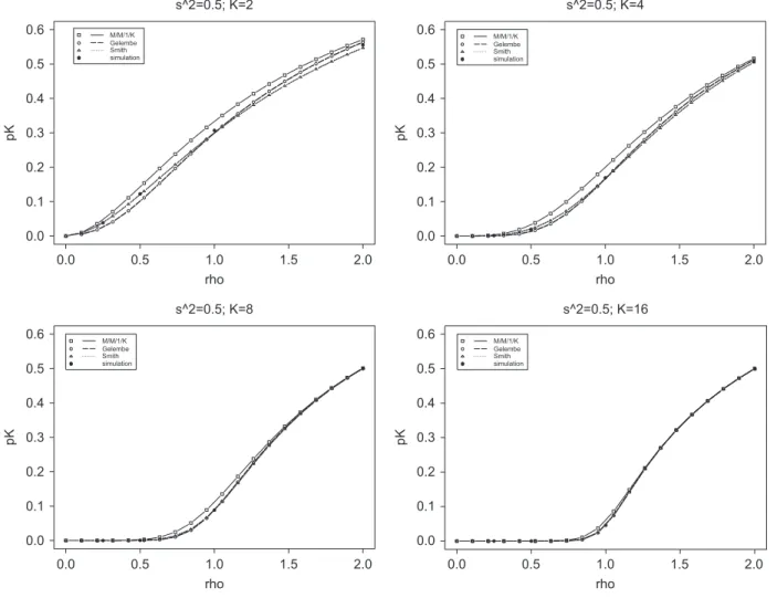
Fig. 3. Comparisons forpKfor hypoexponential systems withc2s=0.5.

probability of singleM/G/1/Kqueues

pK₌

((2+√c2s−√+2(K−1))/(2+√c2s−√))₍₋₁₊₎

(2(2+√c2

s−√+(K−1))/(2+√c2s−√))₋₁

. (12)

As it will be seen in the following sections, Eq. (12) will be useful for computing performance measures of queueing networks ofM/G/1/Ksystems.

3.4. Computational experiments

rho

pK

0.0 0.5 1.0 1.5 2.0

s^2=2.0; K=2

rho

pK

0.0 0.5 1.0 1.5 2.0

s^2=2.0; K=4

rho

pK

0.0 0.5 1.0 1.5 2.0

s^2=2.0; K=8

rho

pK

0.0 0.5 1.0 1.5 2.0

s^2=2.0; K=16 0.6

0.5

0.4

0.3

0.2

0.1

0.0

0.6

0.5

0.4

0.3

0.2

0.1

0.0

0.6

0.5

0.4

0.3

0.2

0.1

0.0

0.6

0.5

0.4

0.3

0.2

0.1

0.0

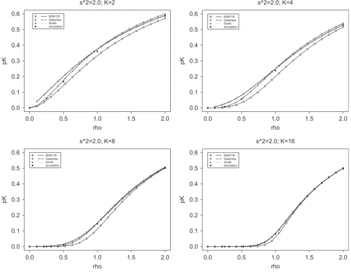
Fig. 4. Comparisons forpKfor hyperexponential systems withc2s=2.0.

3.4.1. Markovian systems

Results for the first set of experiments, done for Markovian systems, that is,c2_s=1.0, are presented inFig. 2. These experiments were performed to validate the implementations as all of them should yield the same results, which they indeed do in most of the cases. Actually, only forK₌2 and<1.0 divergences were noticed involving Gelenbe’s formula. Notice that asKincreases the blocking probabilities get close to zero when<1.0, which is a logical and expected behavior.

3.4.2. Hypoexponential systems

The results for hypoexponential systems, withc2_{s =}0.5, are available inFig. 3. For hypoexponential systems the Markovian approximation is an upper bound for the blocking probabilities, as it always overestimates the simulation results, assumed here as reference. Thus, it is clear that by simply using Markovian approximations for hypoexponential systems one will tend to allocate larger buffer spaces than necessary.

3.4.3. Hyperexponential systems

Results for hyperexponential systems, withc_s2₌2.0, are presented inFig. 4. The Markovian approximations may be seen as a lower bound for the blocking probabilities, as their values always underestimate the simulation results, taken here as references. The inadequacy of Markovian approximations for hyperexponential systems for optimal buffer allocation purposes is confirmed. In this case, one will allocate less buffer space than necessary.

In comparison with the simulations results, Gelenbe’s approximations overestimate the blocking probabilities just in the most appropriate range of(for system utilization less than unity,<1.0). By its side, MacGregor Smith’s approximation presents estimates close to the simulation results independent of. As observed for hypoexponential systems, the blocking probabilities tend to be close to zero for system utilization below unity as the buffer size increases. Also similarly to hypoexponential systems, all approximations tend to agree for larger buffer size systems.

4. Performance evaluation algorithm

4.1. Generalized expansion method

Notice that, in order to solve the optimization problem given by Eqs. (1)–(3), one will need an estimate for the throughput,(x). An algorithm available is the GEM, successfully used in the past to estimate performance measures for arbitrarily configured finite queueing networks.

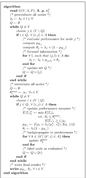
Well described in many articles, in particular in the recently published article by Kerbache and MacGregor Smith [21], the GEM is basically a combination of node-by-node decomposition and repeated trials, in which each queue is analyzed separately and then corrections are made in order to take into account the interrelation between the queues in the network. The GEM uses type I blocking, that is, the upstream node gets blocked if the service on a customer is completed but it cannot move downstream due to the queue at the downstream node being full. This is sometimes referred to as blocking after service, which is prevalent in most production and manufacturing, transportation, and similar systems. The implementation used here in this work is based on a recently proposed implementation of the GEM by Cruz and MacGregor Smith[2], suitable for light to moderate traffic, and, for the first time, used in networks ofM/G/1/Kqueues. The algorithm may be seen inFig. 5.

The GEM starts by reading all relevant information from the network under analysis, including the set of vertexes in the networks,V, the set of arcs,A, and the routing matrix,P _{≡ [}p(i,j )], which defines the probabilities of an entity to choose one or another path. Following Kerbache and MacGregor Smith[21], the GEM consists of creating for each finite queue following another finite queue (seeFig. 6), represented by vertexj, an auxiliary vertexhj, modeled as an

M/G/_∞queue. When an entity arrives at the system, vertexjmay be blocked with probabilitypKj, or unblocked, with probability(1−pKj). Under blocking, the entities are rerouted to vertexhjfor a delay while nodejis busy. Vertex

hjhelps to accumulate the time an entity has to wait before entering vertexjand to compute the effective arrival rate to vertexj.

Thus, the algorithm chooses an arbitrary node,j, from setVbut not from setQ(in whichQis the set of nodes already evaluated), such that for all arc(i, j )_∈A, vertexihas been evaluated already. Then, vertexjhas computed its blocking probabilitypKj, from Eq. (12), and its arrival rate, fromj=j×(1−pKj),j=j+

iij. These service rates are then forwarded as arrival rates to the downstream nodes (if they exist), and vertexjis included into setQ. For instance, in the network illustrated inFig. 1, a possible valid sequence to perform pre-evaluations is 1_→2_→4_→3_→5_→6. Notice that the GEM also includes a re-evaluation step, designed to guarantee flow conservation, that is,jj +

∀i|(i,j )∈Aipij, for allj ∈ V. The re-evaluation step is a labeling algorithm working in reverse. For the network presented inFig. 1, a possible valid sequence to perform the re-evaluations is 6_→5_→4_→3_→2_→1, because a node can only be re-evaluated if all of its successors were re-evaluated already. The re-evaluation algorithm corrects the estimates by means of adjustments in the expected service time of each nodei,E_[Ts]i. Further details will not be given in this article. The interested reader is referred to Cruz and MacGregor Smith[2].

4.2. Computational experiments

Fig. 5. Algorithm for performance evaluation.

Table 1

Results for the generalized expansion method

c2_s Node #1 Node #2 Node #3

Analytical Simulation % Analytical Simulation % Analytical Simulation % CPUa

Series topology:

0.1 0.5 0.9783 0.9928 0.0011 1.5 0.9783 0.9928 0.0011 1.5 0.9783 0.9928 0.0011 1.5 1.63 1.0 0.9737 0.9910 0.0008 1.7 0.9737 0.9910 0.0008 1.7 0.9737 0.9910 0.0008 1.7 1.68 2.0 0.9643 0.9873 0.0008 2.3 0.9643 0.9873 0.0008 2.3 0.9643 0.9873 0.0008 2.3 1.68 0.2 0.5 1.8530 1.9477 0.0018 4.9 1.8530 1.9477 0.0018 4.9 1.8530 1.9477 0.0018 4.9 3.38 1.0 1.8225 1.9348 0.0013 5.8 1.8225 1.9348 0.0013 5.8 1.8225 1.9348 0.0013 5.8 3.42 2.0 1.7675 1.9072 0.0011 7.3 1.7675 1.9072 0.0011 7.3 1.7675 1.9072 0.0011 7.3 3.38 0.4 0.5 3.1667 3.6389 0.0014 13.0 3.1667 3.6389 0.0014 13.0 3.1667 3.6389 0.0014 13.0 6.75 1.0 3.0333 3.5522 0.0014 14.6 3.0333 3.5522 0.0014 14.6 3.0333 3.5522 0.0014 14.6 6.62 2.0 2.8324 3.3890 0.0019 16.4 2.8324 3.3890 0.0019 16.4 2.8324 3.3890 0.0019 16.4 6.42

Split topology:

1.0 0.5 0.9904 0.9930 0.0010 0.3 0.5939 0.5959 0.0008 0.3 0.3965 0.3970 0.0006 0.1 1.37 1.0 0.9884 0.9912 0.0010 0.3 0.5926 0.5946 0.0008 0.3 0.3958 0.3966 0.0007 0.2 1.43 2.0 0.9842 0.9873 0.0009 0.3 0.5899 0.5925 0.0008 0.4 0.3943 0.3948 0.0007 0.1 1.40 2.0 0.5 1.9322 1.9479 0.0017 0.8 1.1569 1.1682 0.0011 1.0 0.7754 0.7797 0.0010 0.6 3.17 1.0 1.9173 1.9352 0.0014 0.9 1.1474 1.1608 0.0009 1.2 0.7699 0.7744 0.0009 0.6 2.85 2.0 1.8892 1.9121 0.0012 1.2 1.1296 1.1469 0.0009 1.5 0.7596 0.7653 0.0009 0.7 2.83 4.0 0.5 3.5683 3.6475 0.0020 2.2 2.1269 2.1884 0.0013 2.8 1.4414 1.4591 0.0010 1.2 5.90 1.0 3.4851 3.5778 0.0016 2.6 2.0747 2.1467 0.0011 3.4 1.4105 1.4310 0.0011 1.4 5.50 2.0 3.3506 3.4542 0.0017 3.0 1.9904 2.0725 0.0012 4.0 1.3602 1.3817 0.0009 1.6 5.48

Mere topology:

1.0 0.5 0.3995 0.3990 0.0007 ₋0.1 0.5910 0.5986 0.0011 1.3 0.9904 0.9976 0.0015 0.7 1.05 1.0 0.3994 0.3995 0.0008 0.0 0.5890 0.5977 0.0009 1.4 0.9884 0.9972 0.0011 0.9 1.07 2.0 0.3992 0.3991 0.0006 0.0 0.5850 0.5966 0.0011 1.9 0.9842 0.9957 0.0012 1.2 1.08 2.0 0.5 0.7961 0.7956 0.0010 ₋0.1 1.1361 1.1875 0.0010 4.3 1.9322 1.9831 0.0014 2.6 2.28 1.0 0.7953 0.7948 0.0013 ₋0.1 1.1220 1.1843 0.0012 5.3 1.9173 1.9792 0.0021 3.1 2.25 2.0 0.7936 0.7920 0.0010 −0.2 1.0955 1.1763 0.0013 6.9 1.8891 1.9683 0.0016 4.0 2.23 4.0 0.5 1.5718 1.5682 0.0012 −0.2 1.9962 2.3034 0.0014 13.3 3.5681 3.8716 0.0019 7.8 4.68 1.0 1.5655 1.5575 0.0010 −0.5 1.9191 2.2737 0.0013 15.6 3.4845 3.8312 0.0017 9.0 4.60 2.0 1.5530 1.5334 0.0012 −1.3 1.7960 2.2165 0.0012 19.0 3.3490 3.7499 0.0012 10.7 4.52

a_{Simulation CPU time in minutes.}

units were used as the simulation times with a warm-up period of 2000 time units. The simulation results presented are the averages over 20 replications, to get reduced mean standard errors. Slightly longer and shorter simulations and replications were tested but the results (not shown) did not change significantly.

Table 1presents the results for the experiments, obtained from a PC Pentium(R) 4 CPU 3.00 GHz, 960 MB RAM running the Microsoft(R) Windows XP. In the column labeled ‘analytical’, we give the throughput result from the GEM for each of the cases. We then compare this analytical result with the average result obtained via the simulation. The column refers to the half-width of the 95% confidence interval. Notice that the Monte Carlo errors were quite small. Also included in these tables is the % deviation for the analytical results on the throughput, column%, from which we can see that the analytical results may be quite far away from the simulation (exact) results (see results in boldface inTable 1). Mainly the results from this GEM implementation get worse as the system gets overloaded. Notice that for the split topology the results are quite good, because the flow in excess is rejected right away in the first node being then divided into two nodes with equal service rate. It appears that the quality of the approximations is mainly dependent on the squared coefficient of variation of the service time. In fact, the % deviation finds its highest values with the highestc_s2.

Concluding, from the simulation CPU times reported for a single evaluation of the performance measures for the queueing networks, it is apparent that simulation-based techniques may not be quite effective for optimization purposes of these queueing networks, unless the system is very small, because typically hundreds or thousands of performance evaluations may be required for the optimization algorithms. On the other hand, the analytical results are shown to be quite reliable and satisfactory. Additionally, as this new implementation of the GEM is primarily for optimization purposes, we should not worry too much about high deviations under overloaded traffic.

5. Buffer allocation algorithm

5.1. A Lagrangian relaxation approach

The optimization problem that will be examined here is given by Eqs. (1)–(3). In the formulation,xi becomes the decision variable under optimization control, that is,xi ≡K, for theith queue.

A possible way to solve the problem is through Lagrangian relaxation, a technique that consists in relaxing the complicating constraints and including then in the objective function as a penalty. Among the classical references to the Lagrangian relaxation, the article by Fisher[22]should be cited. A recently published tutorial about the Lagrangian relaxation by Lemaréchal[23]is another reference for the technique. One way to incorporate the throughput constraint is then through a penalty function. Defining a dual variableand relaxing the constraint (2), the following penalized problem is given:

L()=min ⎡

⎢ ⎣

N

i=1

xi+(min−(x))

0 ⎤

⎥

⎦ (13)

s.t.

xi ∈N, ∀i,

0.

Note that for any feasible vectorx—that is, a vectorxfor which the constraints (2) and (3) hold—the term(min−

(x))must be non-positive and will be a penalty of the objective function related to the difference between the threshold throughput,min, and the effective throughput,(x). Thus, it follows thatL()Z, that is,L()is an inferior limit forZ, the optimal solution for the BAP, since removing the constraint (2) cannot increase the optimal valueZ(for a detailed discussion on this issue, the reader is referred to the article by Fisher[22]).

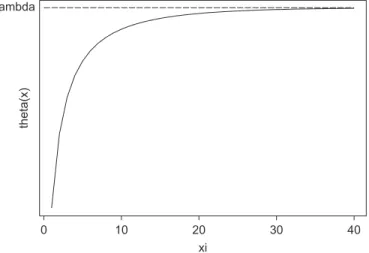
xi

theta(x)

0 10 20 30 40

lambda

Fig. 7. Throughput versus buffer size.

alpha

L(alpha)

0 100 200 300 400

40

30

20

10

0

Fig. 8. Lagrangian functionL().

Theorem 1. Ifminis exactly the total external arrival rate,then the highest inferior limit,L(∗)₌max0L(), is achieved for∗−→ ∞.

Proof. It follows from(x)being a non-decreasing function ofx, as it is seen inFig. 7, and also from the Lagrangian function,L(), which is the minimum of linear functions of,

L()₌min ⎛

⎜ ⎜ ⎜ ⎜ ⎜ ⎝

N

i=1 xi

intercept

+

slope

(min₋(x)) ⎞

⎟ ⎟ ⎟ ⎟ ⎟ ⎠ ,

with non-negative intercepts and non-negative slopes with

lim x→∞(

min

−(x))₌0,

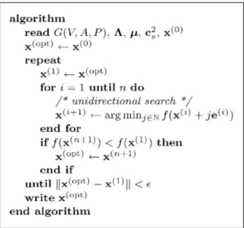
Fig. 9. Algorithm for optimal buffer allocation.

The best Lagrangian multiplier, as defined by Theorem 1, is not practical because one would need that

(min−(x))₌0,

which yieldsxi → ∞,∀i. On the other hand, if a small difference, say(min−(x))=ε, is acceptable, it must hold that

(min−(x))1,

because, otherwise, it would be better to spend one more unity of buffer space to someith queue,xi, to increase(x) (remind that(x)is a non-decreasing function ofx). Thus, it is possible to define a correspondingεas follows:

ε 1

(min₋(x)),

which, assuming(min₋(x))10−3_{, yieldsε}

=103.

5.2. Search algorithm

The Lagrangian relaxation of the BAP,L(), plus an additional relaxation of the integrality constraints forxi, is a classical unconstrained optimization problem. Among all possible algorithms to solve the BAP, a derivative free search algorithm was used, which is shown inFig. 9, for its simplicity, and also efficiency, as it will be seen.

The algorithm starts by reading the inputs, that is, the number of vertexes in the networks,V, the number of arcs,A, the routing matrixP _{≡ [}p(i,j )], which defines the probabilities of an entity to choose one or another path. Also read are the vector of external arrival rates,, service rates,µ, squared coefficient of variation of service rates,c2_s, and an

initial buffer allocation vector,x(0)_{. With these values, the algorithm takes the objective function}

f (x)₌ N

i=1

xi₊(min₋(x)),

which is optimized only in relation to the first coordinate of vectorx, keeping fixed the remaining coordinates. The process is repeated for the second coordinate and so on, until the last coordinate is reached. A completely new vector

6. Experimental results

All algorithms were implemented in FORTRAN, taking advantage of the subroutines already developed for similar problems[1,19]and are available upon request. The experiments were run for tandem, split, and merge queues, as presented inFig. 10.

The arrival rates considered were₌min_{= {}1.0,2.0,4.0_}, the service rates,_i=10.0,_∀i, resulting in a system utilization_{= {}0.1,0.2,0.4_}, combined with several values for the squared coefficient of variation,c2_{s= {}0.5,1.0,2.0_}, and number of nodes,_|V_{| = {}3,7,15_}. The results are presented inTable 2.

FromTable 2, it is seen that the pattern found in the small networks essentially becomes the pattern for the large networks. Also, the optimal allocation clearly depends on the coefficient of variation,c2_s. The results make sense, are stable, and are symmetrical for the split and merge topologies. Note that the buffer allocation is uniform across the series topology. This type of result is similar to the uniform buffer allocation results of De Kok[24]but the well-known bowl phenomenon[25]was not obtained here. It turns out that the bowl phenomenon is only present in optimal buffer allocations constrained to a maximal number of total buffer allocated, as, for instance, in the model presented in the article by Hiller and So[25].

In order to see how close to optimal the generated patterns are, it is interesting to compare these results with simulation. Experiments with ARENA with 200,000 time units, 2000 time units warm-up and 20 replications were found to yield fairly stable results and short 95% confidence intervals. For all the non-exponential service times, a two-stage gamma distribution was used to capture the general service times with non-unitc2_s. The results for some of the series queues are seen inTable 3.

The result for a three-node series topology was analyzed in more detail. Note that the best solutions correspond closely to the lowestL()(seeTable 3, in boldface). The general conclusion is that optimization algorithm tends to

Table 2

Buffer allocation results

|V| 3 7 15

c2

s K K K

Series topology

0.1 0.5 (3 3 3)a _{(3 3 3 3 3 3 3) (3 3 3 3 3 3 3 3 3 3 3 3 3 3 3)}

1.0 (3 3 3) (3 3 3 3 3 3 3) (3 3 3 3 3 3 3 3 3 3 3 3 3 3 3) 2.0 (4 4 4) (4 4 4 4 4 4 4) (4 4 4 4 4 4 4 4 4 4 4 4 4 4 4) 0.2 0.5 (5 5 5) (5 5 5 5 5 5 5) (5 5 5 5 5 5 5 5 5 5 5 5 5 5 5) 1.0 (5 5 5) (5 5 5 5 5 5 5)a (5 5 5 5 5 5 5 5 5 5 5 5 5 5 5) 2.0 (6 6 6) (6 6 6 6 6 6 6) (6 6 6 6 6 6 6 6 6 6 6 6 6 6 6) 0.4 0.5 (7 7 7) (7 7 7 7 7 7 7) (7 7 7 7 7 7 7 7 7 7 7 7 7 7 7) 1.0 (8 8 8) (8 8 8 8 8 8 8) (8 8 8 8 8 8 8 8 8 8 8 8 8 8 8)

2.0 (10 10 10) (10 10 10 10 10 10 10) (10 10 10 10 10 10 10 10 10 10 10 10 10 10 10)

Split topology

0.1 0.5 (3 3 2) (3 3 2 2 2 2 2) (3 3 2 2 2 2 2 2 2 2 1 2 1 1 1) 1.0 (3 3 2) (3 3 2 2 2 2 2) (3 3 2 2 2 2 2 2 2 2 1 2 1 1 1) 2.0 (4 3 2) (4 3 2 2 2 2 2) (4 3 2 2 2 2 2 2 2 2 1 2 1 1 1) 0.2 0.5 (5 4 3) (5 4 3 3 2 2 2) (5 4 3 3 2 2 2 2 2 2 2 2 2 2 2) 1.0 (5 4 3) (5 4 3 3 3 3 2) (5 4 3 3 2 2 2 2 2 2 2 2 2 2 2) 2.0 (6 4 3) (6 4 3 3 3 3 2) (6 4 3 3 3 3 2 2 2 2 2 2 2 2 2) 0.4 0.5 (7 5 4) (7 5 4 4 3 3 3) (7 5 4 4 3 3 3 3 3 3 2 3 2 2 2) 1.0 (8 6 4) (8 6 4 4 3 3 3) (8 6 4 4 3 3 3 3 3 3 2 3 2 2 2) 2.0 (10 6 5) (10 6 5 5 4 4 3) (10 6 5 5 4 4 3 3 3 3 2 3 2 2 2)

Merge topology

0.1 0.5 (2 3 3) (2 2 2 2 2 3 3) (1 1 1 2 1 2 2 2 2 2 2 2 2 3 3) 1.0 (2 3 3) (2 2 2 2 2 3 3) (1 1 1 2 1 2 2 2 2 2 2 2 2 3 3) 2.0 (2 3 4) (2 2 2 2 2 3 4) (1 1 1 2 1 2 2 2 2 2 2 2 2 3 4)

0.2 0.5 (3 4 5) (2 2 2 3 3 4 5) (2 2 2 2 2 2 2 2 2 2 2 3 3 4 5) 1.0 (3 4 5) (2 2 3 3 3 4 5) (2 2 2 2 2 2 2 2 2 2 2 3 3 4 5) 2.0 (3 4 6) (2 3 3 3 3 4 6) (2 2 2 2 2 2 2 2 2 3 3 3 3 4 6)

0.4 0.5 (4 5 7) (3 3 3 4 4 5 7) (2 2 2 3 2 3 3 3 3 3 3 4 4 5 7) 1.0 (4 6 8) (3 3 3 4 4 6 8) (2 2 2 3 2 3 3 3 3 3 3 4 4 6 8) 2.0 (5 6 10) (3 4 4 5 5 6 10) (2 2 2 3 2 3 3 3 3 4 4 5 5 6 10)

Table 3

Simulation results for tandem queues

c2_s |V| x (x) L() CPUa

Average

1.0 0.5 3 (2 2 2) 0.9928 0.0011 13.19 1.68

(2 2 3) 0.9928 0.0011 14.18 1.67

(2 3 3) 0.9928 0.0011 15.17 1.68

(3 3 3) 0.9994 0.0012 9.59b,c _1.47

(3 3 4) 0.9999 0.0009 10.07 1.70

(3 4 4) 1.0000 0.0009 11.00 1.70

(4 4 4) 1.0000 0.0013 12.00 1.70

2.0 1.0 7 (3 3 3 3 3 3 3) 1.9861 0.0014 34.90 7.27

(4 4 4 4 4 4 4) 1.9966 0.0010 31.40b _7.28

(5 5 5 5 5 5 5) 1.9994 0.0013 35.60c 7.28

(6 6 6 6 6 6 6) 1.9996 0.0016 42.40 7.30

(7 7 7 7 7 7) 2.0001 0.0021 48.90 7.65

a_{CPU time for simulation in ARENA in minutes.} b_{Best solution via simulation.}

c_{Best solution via optimization algorithm.}

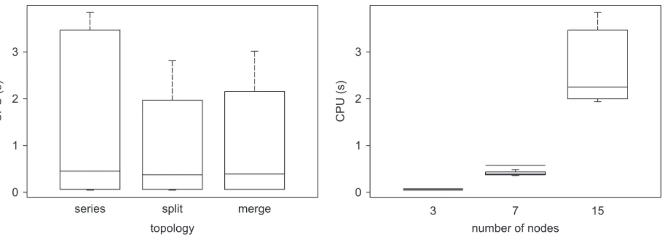
series split merge

topology

CPU (s)

3 15

number of nodes

CPU (s)

0 1 2

3 3

2

1

0

7

Fig. 11. Running times in function of the topology and number of nodes.

allocate more space than necessary to ensure the desired performance. Also noticeable is that the CPU time for the simulations grows quickly as the number of node in the network increases indicating that the simulation may not be the most efficient tool for optimizing but it is certainly useful for assessing the quality of solutions via other methods.

As a final note on the computational performance of the algorithm, it is important to know how it will behave with small changes in the input. The running times, in seconds, for the cases studied inTable 2are presented inFig. 11, reporting boxplots in function of the topology and the number of nodes in the network.

The running times seem to be independent of the topology but they certainly will increase with the number of nodes. This increase, although not too drastic, is followed by an increase in the variability, which indicates that the running times may be less predictable for large networks.

7. Summary and conclusions

when queues are configured in networks, in which blocking after service frequently occurs. In this paper, some of the most effective approximations for the blocking probability, a crucial performance measure for the BAP treated here, were extensively compared. The approximation by MacGregor Smith[19]seemed to be the most accurate for the cases tested and was used here to solve the BAP.

The algorithm proposed is based on a Lagrangian relaxation, a technique that has been proved efficient in solving optimization problems with complicated constraints. The Lagrangian relaxation enables one to avoid hard optimization formulations by relaxing complicating constraints and including then into the objective function as a penalty. Important properties of the relaxed problem were derived, which made possible the development of a search algorithm, consid-erably simpler than the algorithm previously published for the same problem by MacGregor Smith[1]. In comparison with the exact simulation results, the algorithm seemed to produce very fast and accurate solutions and can be used in the design of production systems.

Topics for future research in the area include extensions to systems that have loops, such as systems with cap-tive pallets and fixtures. Also of interest is the study of algorithms for multi-server general service time queueing networks.

Acknowledgments

The research of prof. Frederico Cruz has been partially funded by the CNPq (Conselho Nacional de Desenvolvimento Científico e Tecnológico) of the Ministry for Science and Technology of Brazil, Grants 201046/1994-6, 301809/1996-8, 307702/2004-9, 472066/2004-301809/1996-8, and 472877/2006-2, by the FAPEMIG (Fundação de Amparo à Pesquisa do

Es-tado de Minas Gerais), Grants CEX-289/98 and CEX-855/98, and PRPq-UFMG, Grant 4081-UFMG/RTR/FUNDO/

PRPq/99.

References

[1]MacGregor Smith J, Cruz FRB. The buffer allocation problem for general finite buffer queueing networks. IIE Transactions on Design & Manufacturing 2005;37(4):343–65.

[2]Cruz FRB, MacGregor Smith J. Approximate analysis ofM/G/c/cstate-dependent queueing networks. Computers & Operations Research 2007;34(8):2332–44.

[3]Kimura T. Optimal buffer design of anM/G/s queue with finite capacity. Communications in Statistics-Stochastic Models 1996;12(1): 165–80.

[4]Soyster AL, Schmidt JW, Rohrer MW. Allocation of buffer capacities for a class of fixed cycle production lines. AIIE Transactions 1979;11(2): 140–6.

[5]Baker KR, Powell S, Pyke D. Buffered and unbuffered assembly systems with variable processing times. Journal of Manufacturing and Operations Management 1990;3:200–23.

[6]Spinellis D, Papadopoulos CT, MacGregor Smith J. Large production line optimization using simulated annealing. International Journal of Production Research 2000;38(3):509–41.

[7]Kubat P, Sumita U. Buffers and backup machines in automatic transfer lines. International Journal of Production Research 1985;23(6): 1259–80.

[8]Yamashita H, Altiok T. Buffer capacity allocation for a desired throughput in production lines. IIE Transactions 1998;30(10):883–92. [9]Yamashita H, Onvural R. Allocation of buffer capacities in queueing networks with arbitrary topologies. Annals of Operations Research

1994;48:313–32.

[10]Altiok T, Stidham S. The allocation of interstage buffer capacities in production lines. IIE Transactions 1983;15:251–61.

[11]Hillier FS, So KC. The effect of the coefficient of variation of operation times on the allocation of storage space in production line systems. IIE Transactions 1991;23(2):198–206.

[12]MacGregor Smith J, Chikhale N. Buffer allocation for a class of nonlinear stochastic knapsack problems. Annals of Operations Research 1995;58:323–60.

[13]MacGregor Smith J, Daskalaki S. Buffer space allocation in automated assembly lines. Operations Research 1988;36(2):343–58. [14]Gross D, Harris CM. Fundamentals of queueing theory. 3rd ed, New York: Wiley; 1998.

[15]Springer MC, Makens PK. Queueing models for performance analysis: selection of single station models. European Journal of Operational Research 1992;58(1):123–45.

[16]Gelenbe E. On approximate computer system models. Journal of the ACM 1975;22(2):261–9. [17]Tijms HC. Stochastic modeling and analysis: a computational approach. New York: Wiley; 1986.

[18]Kimura T. A transform-free approximation for the finite capacityM/G/squeue. Operations Research 1996;44(6):984–8. [19]MacGregor Smith J.M/G/c/ kblocking probability models and system performance. Performance Evaluation 2002;52:237–67. [20]Kelton D, Sadowski RP, Sadowski DA. Simulation with ARENA. New York, NY: McGraw-Hill College Division; 2001.

[22]Fisher ML. An application oriented guide to Lagrangian relaxation. Interfaces 1985;15:10–21. [23]Lemaréchal C. The omnipresence of Lagrange. 4OR 1; 2003. p. 7–25.

[24]De Kok AG. Computationally efficient approximations for balanced flowlines with finite intermediate buffers. International Journal of Production Research 1990;28:401–19.