Pesq. agropec. bras., Brasília, v.49, n.3, p.215-224, mar. 2014 DOI: 10.1590/S0100-204X2014000300008 Daniel Fonseca de Carvalho(1),, Valdemir Lucio Durigon(2), Mauro Antonio Homem Antunes(1),
Wilk Sampaio de Almeida(1) and Paulo Tarso Sanches de Oliveira(3)
(1)Universidade Federal Rural do Rio de Janeiro (UFRRJ), Departamento de Engenharia, BR‑465, Km 7, CEP 23897‑000 Seropédica, RJ, Brazil.
E‑mail: [email protected], [email protected], [email protected] (2)UFRRJ, Colégio Técnico, BR–465, Km 8, CEP 23897‑000
Seropédica, RJ, Brazil. E‑mail: [email protected] (3)Universidade de São Paulo, Escola de Engenharia de São Carlos,
Departamento de Engenharia Hidráulica e Sanitária, Caixa Postal 359, CEP 13560‑970 São Carlos, SP, Brazil. E‑mail: [email protected]
Abstract – The objective of this work was to evaluate the seasonal variation of soil cover and rainfall erosivity, and their influences on the revised universal soil loss equation (Rusle), in order to estimate watershed soil losses in a temporal scale. Twenty‑two TM Landsat 5 images from 1986 to 2009 were used to estimate soil use and management factor (C factor). A corresponding rainfall erosivity factor (R factor) was considered for each image, and the other factors were obtained using the standard Rusle method. Estimated soil losses were grouped into classes and ranged from 0.13 Mg ha‑1 on May 24, 2009 (dry season) to 62.0 Mg ha‑1 on
March 11, 2007 (rainy season). In these dates, maximum losses in the watershed were 2.2 and 781.5 Mg ha‑1,
respectively. Mean annual soil loss in the watershed was 109.5 Mg ha‑1, but the central area, with a loss of nearly
300.0 Mg ha‑1, was characterized as a site of high water‑erosion risk. The use of C factor obtained from remote
sensing data, associated to corresponding R factor, was fundamental to evaluate the soil erosion estimated by the Rusle in different seasons, unlike of other studies which keep these factors constant throughout time. Index terms: C factor, rainfall erosivity, remote sensing, soil loss, vegetation index.
Predição da erosão do solo com uso da Rusle e séries
temporais de NDVI do Landsat 5 TM
Resumo – O objetivo deste trabalho foi avaliar a variação estacional da cobertura do solo e da erosividade da chuva e suas influências na equação universal de perda de solo revisada (Rusle), para estimar as perdas de solo em uma microbacia, em escala temporal. Vinte e duas imagens Landsat 5 TM, do período de 1986 a 2009, foram utilizadas para estimar o fator de uso e cobertura do solo (fator C). Para cada imagem, foi considerado o valor de erosividade da chuva correspondente (fator R), e os demais fatores foram obtidos utilizando‑se o método‑padrão da Rusle. As perdas de solo foram agrupadas em classes e variaram de 0,13 Mg ha‑1, em
24/5/2009 (estação seca), a 62,0 Mg ha‑1, em 11/3/2007 (estação chuvosa). Nessas datas, os valores máximos
de perda de solo na bacia foram de 2,2 e 781,5 Mg ha‑1, respectivamente. A perda de solo média anual na bacia
hidrográfica foi de 109,5 Mg ha‑1, mas a área central da bacia, com perdas de aproximadamente 300,0 Mg ha‑1, foi
considerada como de alto risco à erosão pela água. O uso do fator C obtido a partir da técnica de sensoriamento remoto, associado ao fator R correspondente, é fundamental para avaliar as perdas de solo estimadas pela Rusle em diferentes épocas do ano, diferentemente de outros estudos em que estes fatores são mantidos constantes ao longo do tempo.
Termos para indexação: fator C, erosividade, sensoriamento remoto, perda de solo, índice de vegetação.
Introduction
Water erosion is currently one of the main environmental problems for degrading soil and water resources. In addition, it poses a risk to food safety and represents a serious barrier to sustainable development (Telles et al., 2011). Studies on soil use and management in watersheds, especially predictive models, are fundamental to reduce erosive processes.
Models developed to calculate soil erosion can be divided into empirical, conceptual and those based on physical processes (Aksoy & Kavvas, 2005; Kinnell, 2010).
et al., 2011). Annual soil loss is estimated from the combination of the six factors contained in Rusle: rainfall erosivity (R); soil erodibility (K); slope length (L); slope steepness (S); soil use and management (C); and support practices (P). According to Risse et al. (1993), topography factors (LS) and the C factor exert the greatest influence on the global model efficiency.
The C factor corresponds to soil loss under specific cropping conditions, in relation to that occurring in bare soil (Wischmeier & Smith, 1978). It ranges from 0 (high plant cover) to 1 (bare soil). The Rusle uses five subfactors to calculate the C factor: residual effect of soil use (soil management); soil cover by plant canopy; soil cover by crop residues; roughness of soil surface; and soil moisture (Renard et al., 1997). The evaluation of each subfactor, however, is difficult because of the many possible combinations, and the time spent with data acquisition and analysis (Schönbrodt et al., 2010). Constant values of the Rusle C factor, produced
in earlier studies, are usually used to evaluate soil
erosion in watersheds. These values, however, do not accurately represent vegetation variation, particularly in large areas, which can result in mistaken estimates of soil loss (Asis & Omasa, 2007).To avoid this problem, some studies have attempted to estimate the C factor from remote sensing information (Asis & Omasa, 2007; Schönbrodt et al., 2010; Bargiel et al., 2013).
The normalized difference vegetation index (NDVI) is one of the main indices used for vegetation monitoring and assessment, which allows the monitoring of the surface spatial and temporal changes. Therefore, from NDVI values, some methods have been developed to estimate the Rusle C factor (Knijff et al., 1999; Asis & Omasa, 2007; Durigon et al., 2014). These methods are developed from regression models which correlate C factor values, either measured in the field or obtained
from other studies, to NDVI values generally obtained
from TM sensor on Landsat 5, or by the moderate resolution imaging spectroradiometer (Modis) data (Schönbrodt et al., 2010; Le et al., 2012; Alexandridis et al., 2013; Bargiel et al., 2013). However, under
tropical climate conditions, the C factor tends to be higher than that calculated by these methods for the same vegetation cover. Therefore, a new method for calculating the Rusle C factor, based on NDVI rescaling, was proposed by Durigon et al. (2014). This method produces realistic values for Rusle C factor and is recommended to be used in tropical regions.
The objective of this work was to evaluate the seasonal variation of soil cover and rainfall erosivity,
and their influences on the revised universal soil loss equation (Rusle), in order to estimate watershed soil losses in a temporal scale.
Materials and Methods
This work was carried out from March 2009 to February 2011, at the Palmares‑Ribeirão do Saco watershed, located in the south of the state of Rio de Janeiro, Brazil. The watershed is delimited from 22º22'53"S to 22º30'33"S, and from 43°20'50"W to 43º30'15"W, and its topography is mostly rugged. The climate corresponds to Köppen’s classification of Cw, with temperatures ranging from 12 to 30ºC, and annual rainfall from 1,100 to 1,700 mm. The area was selected because of the spatial diversity of plant cover and the variety of soil classes and slope.
Orthometric altitude digital elevation model (DEM) of the watershed was obtained from two topographic maps, at a scale of 1:50,000 produced by the Instituto Brasileiro de Geografia e Estatística (IBGE) in universal transverse mercator (UTM) projection. A soil map produced by Embrapa Solos (Centro Nacional de Pesquisa de Solos), based on a semi‑detailed survey at a 1:20,000 scale was imported to the ArcGIS, where each mapping unit was reclassified to the second categorical level (suborder), according to the Brazilian soil classification system (SiBCS).
The Rusle model (Renard et al., 1997) was applied to predict soil losses. It uses different procedures from Usle (Wischmeier & Smith, 1978), to determine some parameters: erosivity (R) is calculated in fifteen‑day periods; and slope length (L) should be discretized to better characterize steep slope, as follows: A = R K L S C P, in which: A is the annual mean soil loss (Mg ha‑1 per year); R is the rainfall erosivity
factor (MJ mm ha‑1 h‑1); K is the soil erodibility
factor (Mg ha h MJ‑1 mm‑1); L is the slope length
factor, dimensionless; S is the slope steepness factor, dimensionless; C is the soil use and management factor, dimensionless; and P means the dimensionless factor for conservation practices.
From 1986 to 2000, the erosivity index (EI30)
Pesq. agropec. bras., Brasília, v.49, n.3, p.215‑224, mar. 2014 DOI: 10.1590/S0100‑204X2014000300008
using rainfall data from a meteorological station located in the study area. From 2001 to 2009, data from a pluviograph installed in another meteorological
station located in the watershed was used to obtain the
EI30. In this case, rainfall records showed time intervals
of 10 min. Finally, the R factor was determined as the
summation of EI30 for the corresponding time period.
Chuveros’s software, according to Montebeller et al. (2007), was used to compute the kinetic energy of each rainfall segment using the equation suggested by Foster et al. (1981), and converting data to the international system of units (SI), as follows: Ke = 0.0119 + 0.0873 logI, in which: Ke is the kinetic energy per mm of rainfall (MJ ha‑1 mm‑1); and I is the
rainfall intensity (mm h‑1).
Ke was then multiplied by the rainfall depth in each segment. The values for a same rainfall event were then summed, resulting in the total kinetic energy (Ke, MJ ha‑1) of each rainfall event. The
erosivity index (EI30, MJ mm ha‑1 h‑1), calculated for
each erosive rainfall event, was the product of the total kinetic energy and maximum rainfall intensity in
30 min (I30, mm h‑1). The sum of many EI30 indices,
previously calculated for each rainfall event, allowed determining erosivity indices for every fifteen‑day period. To apply the soil loss model, the adopted R
factor corresponded to EI30 indices calculated for
four‑month periods, including two months before and two months after image acquisition. This procedure was employed to estimate soil loss in the analyzed 22 images, since soil cover did not exhibit a wide variation over the considered period.
Soil erodibility (K factor) in the watershed, expressed in Mg ha h MJ‑1 mm‑1, was estimated according to
Handbook 703 of Rusle (Renard et al., 1997). It was
calculated for each soil class in the watershed as
K = [2.1×10⁴(12 ‑ OM)M1.14 + 3.25(s ‑ 2) + 2.5(p ‑ 3)]/
7.59 × 100, in which: OM is the organic matter content
(dag kg‑1); M is the dimensionless parameter for soil
texture; s is the dimensionless soil structure class; p is the dimensionless parameter which depends on the profile permeability (Pe).
Data on soil organic matter, texture and structure were obtained from a semi‑detailed survey of soil types conducted in the study area by Embrapa. In addition, soil samples were collected in known geographical coordinates, in order to determine macroporosity using the volumetric ring method.
The M parameter was calculated using equation M = (%silt + %fine sand)(100 ‑ %clay) (Wischmeier & Smith, 1978), and profile permeability (Pe) with equation Pe = Po2 (Pizarro, 1978), in which: Po is
the macroporosity percentage. The p parameter of K factor equation, for each soil profile, was calculated after obtained data in profile permeability equation and according to Wischmeier & Smith (1978), using the permeability classification established by the soil survey division staff (1993).
Two topographic maps, with the 1:50,000 scale of Miguel Pereira (SF‑23‑Z‑B‑I‑3) and Vassouras (SF‑23‑Z‑A‑III‑4), were used in this study and included hydrological maps generated by IBGE.
All map layers were transformed from Microstation “dgn” to the ArCGIS “shp” format and imported into the ArcGIS 9.3 software. Then, the units were transformed from kilometers to meters, the layers were georeferenced, and the adjacent vectors of the two topographic maps were joined. All layers of interest, such as hydrography, contours, and land cover, obtained from the various available satellite images, were integrated in the software. Subsequently, the watershed boundaries were demarcated by identifying the drainage divide.
To obtain slope length (L) and slope steepness (S), 10 m spatial resolution DEM, which was previously analyzed to eliminate spurious data, was used. This resolution was chosen by accurately defining flow direction in the watershed, using the “flowdirection” tool of the ArcGIS software. Slope length corresponded to 10.0 m, when water flow was perpendicular to the pixel line, and to 14.14 m when it was diagonally oriented.
The procedure described in Handbook 703 (Renard et al., 1997) was adopted to calculate slope length (L). The landscape was divided into segments, according to the inclination of each slope, as shown below:
L = (λ/72.6)m, in which: m is the slope length exponent
[(m = β/(1 + β))]; and λ is the slope length, in meters; and β = (sin θ/0.0896)/[3(sin θ)0.8 + 0.56], in which: θ is
the slope angle; and β is the rill erosion rate.
Slope steepness factor (S) was also calculated according to Renard et al. (1997), as follows: S = (10.8 × sin θ) + 0.03 for s<9% and S = (16.8 × sin θ) + 0.50 for s ≥ 9%.
(TM sensor), path 217, row 076, from 1986 to 2009. Atmospheric effects on vegetation indices were avoided, by calculating surface reflectance using the 6S model (Antunes et al., 2012). Watershed average altitude (780 m), a tropical gaseous atmosphere, a continental aerosol model, and horizontal visibility (km) of each image were adopted for this atmospheric correction. The images were georeferenced with ground control points, and the NDVI was determined for all images. The NDVI was then used to obtain new images of a rescaled C factor (Cr), as per the following
equation (Durigon et al., 2014): Cr = [(‑NDVI + 1/2)].
Considering the nonexistence of conservation practices in the watershed, the unit value of 1.0 was attributed to the P factor.
Soil loss determined through the Rusle model (Renard et al., 1997), using the ArcGIS software, was classified into four groups of soil loss: 0 to >450.0 Mg ha‑1 (Group 1); 0 to >90.0 Mg ha‑1 (Group 2);
0 to >9.0 Mg ha‑1 (Group 3); 0 to >1.8 Mg ha‑1 (Group
4). Mean soil loss was also estimated using mean values of erosivity and soil cover factor for fifteen‑day periods. The latter was obtained for 24 fifteen‑day periods of each year, using the NDVI from the TM Landsat 5 images above described (Durigon et al., 2014).
Results and Discussion
The differences between the erosivity indices were
significant, with the greatest values obtained in images taken in the rainy season, from December to April (Table 1). In Brazil high values of annual precipitation do not necessarily produce higher values of erosivity because of variation in rainfall intensity (Oliveira et al., 2013b). This way, the greatest erosivity values are generally caused by intense rainfall occurring mainly in the rainy season. Further, Carvalho et al. (2012) found similar results of rainfall erosivity for the same study area.
K factor values in the watershed ranged from
0.0120 to 0.0303 Mg ha h MJ‑1 mm‑1 (Figure 1A). Soil
classes 2 (0.0120 < K < 0.0151) and 3 (0.0151 < K < 0.0154) predominate in the watershed, corresponding to 28.5 and 18.0% of the area, respectively. The highest values were observed in soil classes associated to Ultisol (Argissolo according to SiBCS), except for the Ultisol/Oxisol unit (Argissolo Vermelho‑Amarelo/
Latossolo Vermelho‑Amarelo, SiBCS). The lowest
erodibility values occurred in soil types combining Oxisols (Latossolo Vermelho and Latossolo
Vermelho‑Amarelo, SiBCS). Ultisols usually show
high erodibility values, in contrast to Oxisols. The textural gradient and abrupt texture changes of Ultisols favor erosion because the subsurface horizon exhibits low permeability, facilitating surface runoff of pluvial waters, and ultimately promoting erosion. The more clayey the B horizon, the more difficult the water infiltration and the more severe the erosion process. In an alluvial soil, which consists of complex units of mineral soils, Jebari et al. (2012) recorded erodibility
from 0.036 to 0.054 Mg ha h MJ‑1 mm‑1.
The topography factor (LS) ranged from 0 to 10.83 (Figure 1 b). Values above 6.0 in 48.5% of the watershed area were found. Areas with the highest LS factor values exhibited the highest slope steepness (44.5 to 146.5%). Some studies have concluded that slope steepness rather than slope length affects the value of the topography factor (Van Remortel et al.,
Table 1. Erosivity index values (EI30, in MJ mm ha‑1 h‑1)
corresponding to different images from 1986 to 2009, and regression equations fitted to mean monthly erosivity index (EI30) and monthly rainfall (p, in mm), obtained from the
meteorological station located in Palmares‑Ribeirão do Saco watershed, in the south of Rio de Janeiro state, Brazil.
Image date EI30 Equation for EI30 R2
January 28, 1986 5,394.04 EI30 = 7.100p ‑ 71.66 0.88
May 20, 1986 1,019.03 EI30 = 1.672p + 5.698 0.62
February 24, 1990 2,660.08 EI30 = 1.945p ‑ 5.440 0.74
June 24, 1993 15.68 EI30 = 6.887p ‑ 275.47 0.86
January 18, 1994 4,245.53 EI30 = 7.100p ‑ 71.66 0.88
May 10, 1994 1,986.55 EI30 = 1.672p + 5.698 0.62
October 1, 1994 1,385.66 EI30 = 2.915p ‑ 8.677 0.78
April 11, 1995 1,073.10 EI30 = 18.30p ‑151.2 0.89
June 16, 1996 231.78 EI30 = 6.887p ‑ 275.47 0.86
July 8, 1998 158.31 EI30 = 6.887p ‑ 275.47 0.86
May 24, 1999 41.18 EI30 = 1.672p + 5.698 0.62
July 27, 1999 23.28 EI30 = 6.887p ‑ 275.47 0.86
May 26, 2000 743.38 EI30 = 1.672p + 5.698 0.62
April 27, 2001 2,499.70 EI30 = 18.30p ‑ 151.2 0.89
May 29, 2001 164.20 EI30 = 1.672p + 5.698 0.62
August 1, 2001 37.87 EI30 = 6.887p ‑ 275.47 0.86
July 22, 2003 339.57 EI30 = 6.887p ‑ 275.47 0.86
December 31, 2004 4,345.90 EI30 = 14.30p ‑ 160.7 0.87
March 11, 2007 3,002.17 EI30 = 9.702p ‑ 82.72 0.78
June 15, 2007 21.72 EI30 = 6.887p ‑ 275.47 0.86
August 2, 2007 9.50 EI30 = 6.887p ‑ 275.47 0.86
Pesq. agropec. bras., Brasília, v.49, n.3, p.215‑224, mar. 2014 DOI: 10.1590/S0100‑204X2014000300008
2004; Oliveira et al., 2013a). In addition, several authors have found high LS values (greater than 100) in rugged relief (Yue‑Qing et al., 2009; Kouli et al., 2009).
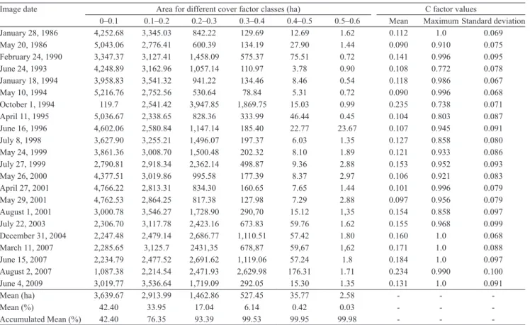
Soil cover classes of higher relevance (0 < Cr < 0.6), for each image used in the study, were
obtained (Table 2). More than 90.0% of the watershed
shows Cr values less than or equal to 0.3, confirming the
predominance of agricultural land use, with permanent plant cover and buildings and bare soil occupying
small patches. The Cr factor values contrast with the
C values of 0 to 0.8767 (Mhangara et al., 2011) and of 0 to 0.5 (Ranzi et al., 2012), which were used to estimate soil erosion in the southernmost portion of South Africa and Northern Vietnam, respectively. This difference is attributed to our approach to determine the C factor (Cr).
The images acquired on 1 October, 1994, and on 2 August, 2007, characterize the dry season in the area,
producing the lowest areas with Cr values in the first
two classes of this factor (0–0.2). The images that revealed the highest areas with plant cover factor in these classes were those obtained on 20 May, 1986, and on 10 May, 1994, both corresponding to the end of the rainy season and onset of the dry season. The highest mean Cr values were found for images
exhibiting the smallest areas in classes 0–0.1 and 0.1–0.2 (Table 2). These values were 0.235 for images taken on 1 October, 1994, and 0.234 for images from
2 August, 2007. On the other hand, a mean Cr value
of 0.090 was obtained for images from 20 May, 1986, and 10 May, 1994. It is highlighted that values of 1.0 can be identified only in specific sites of the watershed and do not reflect a relevant spatial condition, mainly on water bodies where the near infrared reflectance is nearly zero, yielding negative values of NDVI.
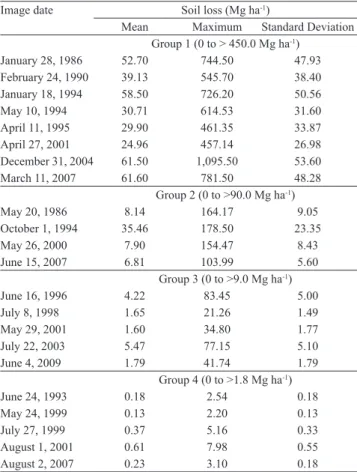
Despite the similarity between the image groups in relation to soil cover, they differ with respect to relative soil loss, primarily because of rainfall erosivity in each period. The rainfall erosivity value (Table 1), used to estimate soil loss from Figure 2 A, was
1,385.67 MJ mm ha‑1 h‑1, and from Figure 2 B, it was
9.50 MJ mm ha‑1 h‑1. These data produced respectively
mean and maximum losses of 35.46 and 178.50 Mg ha‑1
and of 0.23 and 3.10 Mg ha‑1 (Table 3). Therefore,
the difference between erosivity values produced a substantial variation in mean soil loss. However, soil loss differences between Figures 2 C and D are not as pronounced because their erosivity values are similar in comparison to those of Figures 2 A and B. For 20 May, 1986, and 10 May, 1994, mean soil loss was 8.14
and 30.71 Mg ha‑1, and maximum loss was 164.17 and
614.53 Mg ha‑1, respectively (Table 3).
Although Figures 2 A and C correspond to Group 2 (0 to >90 Mg ha‑1 soil loss), the greatest losses have been
found in the image taken on 1 October, 1994, which exhibits the largest area within the classes of higher soil loss. In these situations, rainfall erosivity and soil cover showed a combined effect on the final outcome, since both were higher in Figure 2 A, which resulted in higher losses. This shows that the initial period of rainy season is critical for erosion protection, as soil is more vulnerable, due to low vegetation density.
Images from Group 1 (0 to > 450 Mg ha‑1) were
obtained in the rainy season (December to May), the period of highest erosivity. In these months, soils usually exhibit a higher moisture content, promoting greater runoff and, consequently, soil loss (Ranzi et al., 2012). For this group, the lowest mean soil losses are associated to images from 10 May, 1994, 11 April, 1995, and 27 April, 2001, which also show the lowest rainfall erosivity in Group 1 (Table 1). Although the highest erosivity value of Group 1 was obtained in the image
from 28 January, 1986 (5,394.04 MJ mm ha‑1 h‑1), mean
soil loss in this image was lower than that found in
the other images of this group because of the good soil cover promoted by vegetation. On 28 January, 1986, the watershed area occupied by the 0–0.1 class of the C factor was 4,252.68 ha (Table 2), which is much higher than the value of 1,106.82 ha in the image from 11 March, 2007, which represents the highest mean soil loss in the group. Results shown for the other groups in relation to mean soil loss are homogeneous, except for the image from 1 October, 1994 (Group 2), whose soil loss is greater than that found for some Group 1 images. This image, however, exhibits a higher rainfall
erosivity (1,385.67 MJ mm ha‑1 h‑1) than others from
this group (Table 2). Furthermore, the Cr factors
calculated for this image represented an area of only 119.70 ha (1.4% watershed) in class 0–0.1, whereas for the other images evaluated in this group, the percent areas in class 0–0.1 are 58.7% (20 May, 1986), 51.0% (26 May, 2000) and 26.0% (15 June, 2007). These data explain the difference in soil loss between the 1 October, 1994 image and the others in this group.
Table 2. Soil cover area, and mean and maximum values (with standard deviation) of the C factor obtained from image analysis for Palmares‑Ribeirão do Saco watershed, located in the south of Rio de Janeiro state, Brazil.
Image date Area for different cover factor classes (ha) C factor values
0–0.1 0.1–0.2 0.2–0.3 0.3–0.4 0.4–0.5 0.5–0.6 Mean Maximum Standard deviation
January 28, 1986 4,252.68 3,345.03 842.22 129.69 12.69 1.62 0.112 1.0 0.069
May 20, 1986 5,043.06 2,776.41 600.39 134.19 27.90 1.44 0.090 0.910 0.075
February 24, 1990 3,347.37 3,127.41 1,458.09 575.37 75.51 0.72 0.141 0.996 0.095
June 24, 1993 4,248.89 3,162.96 1,057.14 110.97 3.78 0.90 0.108 0.772 0.078
January 18, 1994 3,958.83 3,541.32 941.22 134.46 8.46 0.54 0.118 0.986 0.067
May 10, 1994 5,216.76 2,752.56 530.64 78.84 5.31 0.72 0.090 0.996 0.068
October 1, 1994 119.7 2,541.42 3,947.85 1,869.75 15.03 0.99 0.235 0.738 0.071
April 11, 1995 5,036.67 2,338.65 828.36 333.99 46.44 0.45 0.104 0.803 0.087
June 16, 1996 4,602.06 2,580.84 1,147.14 185.40 22.77 23.67 0.107 0.945 0.091
July 8, 1998 3,627.90 3,255.21 1,496.07 197.37 6.03 1.35 0.127 0.858 0.080
May 24, 1999 3,861.36 3,008.70 1,500.48 202.32 8.10 1.89 0.121 0.933 0.086
July 27, 1999 2,790.81 2,918.34 2,362.14 498.87 9.36 2.88 0.153 0.952 0.093
May 26, 2000 4,377.51 3,019.86 995.58 177.39 8.37 2.97 0.106 0.921 0.083
April 27, 2001 4,766.22 2,813.31 834.30 160.65 7.65 1.44 0.101 0.996 0.079
May 29, 2001 4,762.53 2,864.25 817.38 127.98 7.29 2.88 0.097 0.956 0.079
August 1, 2001 3,000.78 3,546.27 1,728.90 290,70 15.12 1,35 0.154 0.858 0.097
July 22, 2003 2,306.70 3,117.78 2,423.16 673.83 59.76 1.62 0.155 0.968 0.099
December 31, 2004 2,247.48 2,479.14 2,686.77 1,110.51 57.42 1.80 0.160 1.0 0.068
March 11, 2007 2,285.65 3,125.7 2431,35 678,87 59,67 1,62 0.171 1.0 0.088
June 15, 2007 2,234.79 2,477.52 2,691.62 1,119.06 57.24 1.8 0.184 1.0 0.097
August 2, 2007 1,087.38 2,214.54 2,471.93 2,629.98 176.31 1.71 0.234 0.990 0.100
June 4, 2009 3,019.77 3,536.64 1,719.09 292.05 15.30 1.35 0.131 1.0 0.091
Mean (ha) 3,639.67 2,913.99 1,462.86 527.45 35.77 2.58 ‑ ‑ ‑
Mean (%) 42.40 33.95 17.04 6.14 0.42 0.03 ‑ ‑ ‑
Pesq. agropec. bras., Brasília, v.49, n.3, p.215‑224, mar. 2014 DOI: 10.1590/S0100‑204X2014000300008
For the soil loss class ranging from 0 to >90 Mg ha‑1 (Group 2), we used images from the end
of the rainy season (May, June) and its onset (October). Rainfall in these months usually shows lower depths and intensity, thereby causing lower erosivity. Vegetation in images representing dry season onset (May and June) still shows an adequate soil cover. The highest soil loss was obtained in images from 1 October, 1994, and the lowest on 20 May, 1986. Group 2 images exhibit more homogeneous vegetation than those of Group 1. Images that reflect soil loss in Group 3
(0 to > 9 Mg ha‑1) are also from May, June and July,
which have the lowest rainfall erosivity (154.90 MJ
to 339.57 MJ mm ha‑1 h‑1). In other words, because of
the previous rainy season, soil cover in the watershed is usually more abundant in this period, promoting a good cover, and consequently decreasing soil loss.
The soil cover has a crucial role on the soil erosion
processes in the studied watershed. Some authors have also reported that soil cover has been taken as a key
factor to understand surface runoff and soil erosion in
different management systems in agricultural lands (Panachuki et al., 2011) or in forest studies (Geißler et al., 2012).
As found in class 2, the lowest soil losses (from 0 to
>1.8 Mg ha‑1) were also obtained in images from May
to August, which correspond to the months following the end of the rainy season (Table 2). These losses ranged from 9.50 to 41.18 MJ mm ha‑1 h‑1 year‑1.
The greatest values for annual soil loss are
concentrated in the central watershed area, which holds
the greatest classes of erodibility (K) and topography (LS) factors (Figure 3). The annual soil loss reached 719.97 Mg ha‑1, with mean loss of 109.45 Mg ha‑1.
Figure 2. Soil loss based on the image acquired on October 1, 1994 (A), and on August 2, 2007 (B), on May 20, 1986 (C), and on May 10, 1994 (D), for the Palmares‑Ribeirão do Saco watershed, located in the south of Rio de Janeiro state, Brazil.
N
Soil loss (Mg ha )-1 0.0 0.2
0.4 0.6 0.8 1
1.0 1.2 1.2 1.4 1.4 1.6 1.6 1.8
>1.8
0 0.5 1 2 3 4 5
Km S N W E A B
Soil loss (Mg ha )-1 0 10 20 30 40 50 60 70 80 >90
0 0.5 1 2 3 4 5
km N W S E C
0 0.5 1 2 3 4 5
km N
W
S E Soil loss (Mg ha )-1
0 200 150 100 50 >450 450 350 300 250 D _ _ _ _ _ _ _ _ _ 10 20 30 40 50 60 70 80 90 _ _ _ _ _ _ _ _ _ 50 100 250 150 200 300 350 400 450 _ _ _ _ _ _ _ _ _ 0.6 0.8 0.4 0.2 Soil loss (Mg ha )-1
0 10 10 20 30 40 _ _ _ _ _ 50 40 30 20 50 60 70 80 >90 _ _ _ _ 60 70 80 90
0 0.5 1 2 3 4 5
km N W E
S
The soil loss values corroborate earlier studies carried
out in different regions. Kouli et al. (2009) found mean annual soil loss between 77.2 Mg ha
‑1 and
205.0 Mg ha‑1, in nine watersheds in Greece, with
specific spots exhibiting losses of 4,156 Mg ha‑1.
Yue‑Qing et al. (2009) reported mean annual soil loss of 949.3 Mg ha‑1 in the Maotiao River watershed in
Guizhou, China. These studies were developed in watersheds with some similar features, mainly the agricultural land cover (great C factor), and on rugged relief, which consequently promotes great values of the topographic factor.
In this study, the soil erodibility and rainfall erosivity factors were estimated using adapted models, and
observed soil and rainfall data, while the soil cover factor
was from satellite images. The estimates of these factors
contain unknown uncertainties, and such study would
benefit from time series of soil erosion and sediment yield, which are scarce and difficult to obtain in most cases (Oliveira et al., 2013b). However, soil loss over a long period of time (and a larger area) might be estimated correctly on the basis of the Rusle methodology because overestimations and underestimations can compensate each other, resulting in a good overall assessment of total soil loss (Gabriels et al., 2003). In addition, in the present study, focus is primarily on the evaluation of the
erosivity and soil cover factors, and on seasonality effects
in estimating soil erosion. It was also proposed a method to be applied in watersheds, aiming at evaluating soil erosion risk areas and contributing to conservation plans for water and soil resources. This way, for these aims the method proposed can be applied in other regions with similar conditions.
Conclusions
1. The mean annual soil loss in the evaluated watershed is 109.45 Mg ha‑1; it reaches nearly 300 Mg ha‑1 in the
central portion of the watershed.
2. The use of C factor from remote sensing data, associated to corresponding R factor, is fundamental to evaluate soil erosion estimates by the revised universal soil loss equation (Rusle) in different seasons.
3. It is possible to monitor land cover changes, and to evaluate the effects of seasonality on soil erosion estimates through time series of remotely sensed vegetation index.
4. Over the rainy season, rainfall becomes more intense and, thus, more erosive, but soil cover is gradually recomposed with an increase of canopy density, thereby reducing erosion.
Table 3. Soil loss for the different groups of TM Landsat 5 images analyzed for Palmares‑Ribeirão do Saco watershed, located in the south of Rio de Janeiro state, Brazil.
Image date Soil loss (Mg ha‑1)
Mean Maximum Standard Deviation
Group 1 (0 to > 450.0 Mg ha‑1)
January 28, 1986 52.70 744.50 47.93
February 24, 1990 39.13 545.70 38.40
January 18, 1994 58.50 726.20 50.56
May 10, 1994 30.71 614.53 31.60
April 11, 1995 29.90 461.35 33.87
April 27, 2001 24.96 457.14 26.98
December 31, 2004 61.50 1,095.50 53.60
March 11, 2007 61.60 781.50 48.28
Group 2 (0 to >90.0 Mg ha‑1)
May 20, 1986 8.14 164.17 9.05
October 1, 1994 35.46 178.50 23.35
May 26, 2000 7.90 154.47 8.43
June 15, 2007 6.81 103.99 5.60
Group 3 (0 to >9.0 Mg ha‑1)
June 16, 1996 4.22 83.45 5.00
July 8, 1998 1.65 21.26 1.49
May 29, 2001 1.60 34.80 1.77
July 22, 2003 5.47 77.15 5.10
June 4, 2009 1.79 41.74 1.79
Group 4 (0 to >1.8 Mg ha‑1)
June 24, 1993 0.18 2.54 0.18
May 24, 1999 0.13 2.20 0.13
July 27, 1999 0.37 5.16 0.33
August 1, 2001 0.61 7.98 0.55
August 2, 2007 0.23 3.10 0.18
Annual soil loss (Mg ha yr )-1 -1
0 50 50 100 150 200
250 300 350 400 >450
0 0.5 1 2 3 4 5
km
N
W
S E _
_
_ _
_
_ _
_ _
100 150 200 250
300 350 400 450
Pesq. agropec. bras., Brasília, v.49, n.3, p.215‑224, mar. 2014 DOI: 10.1590/S0100‑204X2014000300008
Acknowledgments
To Coordenação de Aperfeiçoamento de Pessoal de Nível Superior (Capes), for scholarship granted.
References
AKSOY, H.; KAVVAS, M.L. A review of hillslope and watershed scale erosion and sediment transport models. Catena, v.64, p.247‑271, 2005. DOI: 10.1016/j.catena.2005.08.008.
ALEXANDRIDIS, T.K.; SOTIROPOULOU, A.M.; BILAS, G.; KARAPETSAS, N.; SILLEOS, N.G. The effects of seasonality in estimating the c‑factor of soil erosion studies. Land Degradation
and Development, May 2013. DOI: 10.1002/ldr.2223.
ANTUNES, M.A.H.; GLERIANI, J.M.; DEBIASI, P. Atmospheric effects on vegetation indices of TM and ETM+ images from a tropical region using the 6S model. In: IEEE INTERNATIONAL GEOSCIENCE AND REMOTE SENSING SYMPOSIUM, Munich, 2012. Proceedings. Munich: IEEE International, 2012. p.6549‑6552. DOI: 10.1109/IGARSS.2012.6352099.
ASIS, A.M. de; OMASA, K. Estimation of vegetation parameter for modeling soil erosion using linear spectral mixture analysis of Landsat ETM data. ISPRS Journal of Photogrammetry
and Remote Sensing, v.62, p.309‑324, 2007. DOI: 10.1016/j.
isprsjprs.2007.05.013.
BARGIEL, D.; HERRMANN, S.; JADCZYSZYN, J. Using high‑resolution radar images to determine vegetation cover for soil erosion assessments. Journal of Environmental Management,
v.124, p.82‑90, 2013. DOI: 10.1016/j.jenvman.2013.03.049. CARVALHO, D.F. de; KHOURY JÚNIOR, J.K.; VARELLA, C.A.A.; GIORI, J.Z.; MACHADO, R.L. Rainfall erosivity for the state of Rio de Janeiro estimated by artificial neural network.
Engenharia Agrícola, v.32, p.197‑207, 2012. DOI: 10.1590/
S0100‑69162012000100020.
DURIGON, V.L.; CARVALHO, D.F.; ANTUNES, M.A.H.; OLIVEIRA, P.T.S.; FERNANDES, M.M. NDVI time series for monitoring RUSLE cover management factor in a tropical watershed. International Journal of Remote Sensing, v.35, p.441‑453, 2014. DOI: 10.1080/01431161.2013.871081.
FOSTER, G.R.; MCCOOL, D.K.; RENARD, K.G.; MOLDENHAUER, W.C. Conversion of the universal soil loss equation to SI metric units. Journal of Soil and Water
Conservation, v.36, p.355‑359, 1981.
GABRIELS, D.; GHEKIERE, G.; SCHIETTECATTE W.; ROTTIERS, I. Assessment of USLE cover‑management C‑factors for 40 crop rotation systems on arable farms in the Kemmelbeek watershed, Belgium. Soil and Tillage Research, v.74, p.47‑53, 2003. DOI: 10.1016/S0167‑1987(03)00092‑8.
GEIßLER, C.; KÜHN, P.; BÖHNKE, M.; BRUELHEIDE, H.; SHI, X.; SCHOLTEN, T. Splash erosion potential under tree canopies in subtropical SE China. Catena, v.91, p.85‑93, 2012. DOI: 10.1016/j.catena.2010.10.009.
JEBARI, S.; BERNDTSSON, R.; OLSSON, J.; BAHRI, A. Soil erosion estimation based on rainfall disaggregation.
Journal of Hydrology, v.436, p.102‑110, 2012. DOI: 10.1016/j.
jhydrol.2012.03.001.
KINNELL, P.I.A. Event soil loss, runoff and the Universal Soil Loss Equation family of models: a review. Journal of Hydrology,
v.385, p.384‑397, 2010. DOI: 10.1016/j.jhydrol.2010.01.024. KNIJFF, J.M. van der; JONES, R.J.A.; MONTANARELLA L. Soil
erosion risk assessment in Italy. Brussels: European Commission,
1999. 58p.
KOULI, M.; SOUPIOS, P.; VALLIANATOS, F. Soil erosion prediction using the Revised Universal Soil Loss Equation (RUSLE) in a GIS framework, Chania, Northwestern Crete, Greece. Environmental Geology, v.57, p.483‑497, 2009. DOI: 10.1007/s00254‑008‑1318‑9.
LE, Q.B.; TAMENE, L.; VLEK, P.L.G. Multi‑pronged assessment of land degradation in West Africa to assess the importance of atmospheric fertilization in masking the processes involved.
Global and Planetary Change, v.92‑93, p.71‑81, 2012. DOI:
10.1016/j.gloplacha.2012.05.003.
MHANGARA, P.; KAKEMBO, V.; LIM, K.J. Soil erosion risk assessment of the Keiskamma catchment, South Africa using GIS and remote sensing. Environmental Earth Sciences, v.65, p.2087‑2102, 2012. DOI: 10.1007/s12665‑011‑1190‑x.
MONTEBELLER, C.A.; CEDDIA, M.B.; CARVALHO, D.F. de; VIEIRA, S.R.; FRANCO, E.M. Variabilidade espacial do potencial erosivo das chuvas no Estado do Rio de Janeiro.
Engenharia Agrícola, v.27, p.426‑435, 2007. DOI: 10.1590/
S0100‑69162007000300011.
OLIVEIRA, P.T.S. de; ALVES SOBRINHO, T.; RODRIGUES, D.B.B.; PANACHUKI, E. Zoneamento ambiental aplicado à conservação do solo e da água. Revista Brasileira de
Ciência do Solo, v.35, p.1723‑1734, 2011. DOI: 10.1590/
S0100‑06832011000500027.
OLIVEIRA, P.T.S.; RODRIGUES, D.B.B.; ALVES SOBRINHO, T.; PANACHUKI, E; WENDLAND, E. Use of SRTM data to calculate the (R)USLE topographic factor. Acta Scientiarum.
Technology, v.15, p.507‑513, 2013a. DOI: 10.4025/actascitechnol.
v35i3.15792.
OLIVEIRA, P.T.S.; WENDLAND, E.; NEARING, M.A. Rainfall erosivity in Brazil: a review. Catena, v.100, p.139‑147, 2013b. DOI: 10.1016/j.catena.2012.08.006.
PANACHUKI, E.; BERTOL, I.; ALVES SOBRINHO, T.; OLIVEIRA, P.T.S.; RODRIGUES, D.B.B. Perdas de solo e de água e infiltração de água em Latossolo Vermelho sob sistemas de manejo. Revista Brasileira de Ciência do Solo, v.35, p.1777‑1785, 2011. DOI: 10.1590/S0100‑06832011000500032.
PIZARRO, F.C. Drenaje agrícola y recuperación de suelos
salinos. Madrid: Agrícola Española, 1978. 521p.
RANZI, R.; LE, T.H.; RULLI, M.C. A RUSLE approach to model suspended sediment load in the Lo River (Vietnam): effects of reservoirs and land use changes. Journal of Hydrology, v.422, p.17‑29, 2012. DOI: 10.1016/j.jhydrol.2011.12.009.
Equation (RUSLE). Washington: USDA, 1997. 384p. (USDA. Agriculture handbook, 703).
RISSE, L.M.; NEARING, M.A.; NICKS, A.D.; LAFLEN, J.M. Error assessment in the Universal Soil Loss Equation. Soil Science
Society of America Journal, v.57, p.825‑833, 1993. DOI: 10.2136/
sssaj1993.03615995005700030032x.
SCHÖNBRODT, S.; SAUMER, P.; BEHRENS, T.; SEEBER, C.; SCHOLTEN, T. Assessing the USLE crop and management factor C for soil erosion modeling in a large, mountainous watershed in Central China. Journal of Earth Science, v.21, p.835‑845, 2010. DOI: 10.1007/s12583‑010‑0135‑8.
SOIL SURVEY DIVISION STAFF. Soil survey manual. Washington: U.S. Department of Agriculture, 1993. 437p. (USDA. Handbook, 18).
TELLES, T.S.; GUIMARÃES, M. de F.; DECHEN, S.C.F. The costs of soil erosion. Revista Brasileira de Ciência do Solo, v.35, p.287‑298, 2011. DOI: 10.1590/S0100‑06832011000200001. VAN REMORTEL, R.D.; MAICHLE, R.W.; HICKEY, R. J. Computing the LS factor for the Revised Universal Soil Loss Equation through array‑based slope processing of digital elevation data using a C++ executable. Computers and Geosciences, v.30, p.1043‑1053, 2004. DOI: 10.1016/j.cageo.2004.08.001.
WISCHMEIER, W.H.; SMITH, D.D. Predicting rainfall erosion
losses: a guide to conservation planning. Washington: USDA,
1978. 58p. (USDA. Agriculture handbook, 537).
YUE‑QING, X.; JIAN, P.; XIAO‑MEI S. Assessment of soil erosion using RUSLE and GIS: a case study of the Maotiao River watershed, Guizhou Province, China. Environmental Geology,
v.56, p.1643‑1652, 2009. DOI: 10.1007/s00254‑008‑1261‑9.