doi: 10.5540/tema.2018.019.02.0347
The Influence of Velocity Field Approximations
in Tracer Injection Processes
Y.R. N ´U ˜NEZ1, C.O. FARIA2, S.M.C. MALTA3and A.F.D. LOULA3
Received on December 14, 2017 / Accepted on March 19, 2018
ABSTRACT. Although the concentration is the most important variable in tracer injection processes, an efficient and accurate velocity field approximation is crucial to obtain a good physical behaviour for the problem. In this paper we analyse a Stabilized Dual Hybrid Mixed (SDHM) method to solve the Darcy’s system in the velocity and pressure variables that involves the conservation of mass and Darcy’s law. This approach is locally conservative, free of compromise between the finite element approximation spaces and capable of dealing with heterogeneous media with discontinuous properties. The tracer concentration is solved via a combination of the Streamline Upwind Petrov-Galerkin (SUPG) method in space with an im-plicit finite difference scheme in time. We also employ a semi-analytical approach (Abbaszadeh-Dehghani analytical solution) to integrate the transport equation. A numerical comparative study using the SDHM formulation, the Galerkin method and a post-processing technique to calculate the velocity field in combi-nation with those concentration approximation methodologies are presented. In all comparisons, the SDHM formulation appears as the most efficient, accurate and almost free of spurious oscillations.
Keywords: Miscible displacements, Hybridized method, Oil reservoir simulations
1 INTRODUCTION
Information extracted from tracer breakthrough profiles at production wells plays an impor-tant role in reservoir engineering both in the characterization of reservoir heterogeneities as in the project of recovery techniques. Those profiles can be detected either experimentally or via the solution of a mathematical model, which describes the transport of substances through a porous medium. Although the concentration is the variable of most interest, approximation of the velocity field is crucial, since it is responsible for the flow displacement.
*Corresponding author: Cristiane Oliveira Faria – E-mail: [email protected]
1Instituto de Ciˆencias Exatas, UFF, Universidade Federal Fluminense, Rua Desembargador Ellis Hermydio Figueira, 783, 27213-145, Volta Redonda, RJ, Brasil. E-mail: [email protected]
2Instituto de Matem´atica e Estat´ıstica, UERJ, Universidade do Estado do Rio de Janeiro, Rua S˜ao Francisco Xavier, 524, 20550-900, Rio de Janeiro, RJ, Brasil. E-mail: [email protected]
Standard Mixed Finite Element (MFE) methods have been extensively employed during the last decades to solve Darcy’s system [27, 7, 8, 15, 13]. The main idea of these methods is simul-taneously approximate pressure and velocity by using different spaces for each variable. This leads to a compatibility condition between the approximation spaces (the LBB condition [6]), and thus restricts the choice of stable finite element spaces. However, these choices are usu-ally unstable with standard dual mixed formulation, as was illustrated in [11]. A very common example of stable mixed method is given by the Raviart-Thomas spaces [27]. To overcome the compatibility conditions, some stabilized mixed finite element methods were proposed in [16, 19, 22, 4, 10, 11, 12, 5]. In general, these stabilized formulations use continuous Lagrangian finite element spaces and can be successfully employed in simulating Darcy flows in homoge-neous porous media. However, continuous interpolations are not appropriate to heterogehomoge-neous porous media with discontinuous properties. This is due to the fact that on the interfaces of the discontinuities the normal component of Darcy velocity must be continuous (mass conservation) but the tangential component is discontinuous. Formulations based on continuous Lagrangian in-terpolation for velocity fail to represent the tangential discontinuity, producing inaccurate approx-imations and spurious oscillations. Therefore, based on hybridization techniques the Stabilized Dual Hybrid Mixed (SDHM) method that combines advantages of the Discontinuous Galerkin (DG) methods [28] with reduced computational was developed for calculating accurate velocity fields to miscible displacements in homogeneous and heterogeneous porous media [23, 24, 25]. The SDHM formulation consists of a set of local problems defined at the element level coupled to a global system for the Lagrange multipliers. Stabilization terms are added to generate a stable and adjoint consistent formulation allowing greater flexibility in the choice of the approximation spaces. The Lagrange multiplier is identified as the pressure trace on the element interface, which is a natural choice.
In [24] the authors have shown that for regular solutions the SDHM method leads to optimum rates of convergence for the velocity and pressure fields, even when same order interpolations are employed. In addition, the mixture transport in homogeneous and heterogeneous media were recently analysed [25] by studying the influence of the mobility ratio and the permeability field variation. In these cases, the SDHM method was applied in the approximation of the velocity field coupled to the SUPG method in the calculation of the concentration field. The good performance of this methodology was verified through the presented numerical simulations.
The outline of this work is as follows. Section 2 considers the mathematical model of the prob-lem. The stabilized dual hybrid mixed (SDHM) method for the Darcy’s system is presented in Section 3. Tracer concentration approximations based on the SUPG approach and on the semi-analytical methodology are discussed in Section 4, as well as its combination with the usual Galerkin method and a post-processing technique. Numerical experiments are reported in Section 5. Finally, some conclusions are given in Section 6.
2 THE MODEL PROBLEM
The equations governing tracer flows in miscible displacements [26] can be described by the first order system of partial differential equations in the Darcy velocityu=u(x,t)and the pressure
p=p(x)coming from the mass conservation of the mixture and the Darcy’s law:
divu= f in Ω ×(0,T), (2.1)
u=−K∇p in Ω ×(0,T), (2.2)
combined with a convection dominated diffusion-convection equation, which expresses the con-servation of mass of the injected fluid (the tracer concentration equation), c=c(x,t), gives by
φ∂c
∂t +u·∇c−div(D∇c) =g inΩ×(0,T), (2.3)
with the following initial and boundary conditions
c(x,0) = c0(x) in Ω, (2.4)
D∇c·n=0 on ∂Ω×(0,T), (2.5)
u·n=0 on ∂Ω×(0,T). (2.6)
In (2.1-2.6)K=K(x)is the permeability tensor andφis the porosity. Functions f andgare the source terms,nis the exterior normal to∂Ωand
D=D(u) = αmol+αt|u|
I+αl−αt
|u| u⊗u (2.7)
is the dispersion-diffusion tensor [26] whereαmol,αl andαt are the molecular diffusion, lon-gitudinal and transversal dispersion coefficients, respectively, with the domainΩ⊂Rn,∂Ωits boundary andT∈R,T >0.
3 THE HYBRID METHOD FOR DARCY FLOW PROBLEM
LetTh={K}be a regular finite element mesh on the domainΩ
Ω=S
K
K
. The set of all
edges of all elementsK isEh={e:e is an edge o f K f or allK ∈Th}withE0
set of the interior edges. To introduce the hybrid formulation we first multiply equations (2.1)-(2.2) by their respective weighting functions and integrate by parts on each elementK, getting
the following local weak form
(K−1u,v)K −(p,divv)K +
Z
∂K p(
v·nK)ds=0, ∀v∈UK, (3.1)
−(divu,q)K + (f,q)K =0, ∀q∈QK. (3.2)
UK ={v∈L2(K)2,divv∈L2(K),∀K ∈Th}andQK =q∈L2(K),∀K ∈Th are
the local function spaces on each elementK. For each elementK ∈Th,(w,v)K =R
K w vdK
denotes the usualL2(K)inner product,∂K is set of all edges of elementK andnK is the
external normal to∂K.
For a givenp=p¯on∂K, we can solve the set of local problems:
For eachK ∈Th, find{u,p} ∈UK ×QK,∀ {v,q} ∈ UK ×QK such that
(K−1u,v)K −(p,divv)K −(divu,q)K =−(f,q)K −
Z
∂K p(¯
v·nK)ds.
Following the ideas of Arnold et al. [2], an approximation for the pressure trace, ¯p, can be ob-tained by solving a global problem associated with the dual hybrid mixed formulation. Defining the function spacesM ={µ∈L2(e), ∀e∈Eh}, U =∏K UK andQ=∏K QK the dual
hybrid formulation consists in:
Findu∈U,p∈Qandλ∈M, such that
∑
K∈Th
(K−1u,v)K −(p,divv)K +
Z
∂K λ(
v·nK)ds
=0,∀v∈U, (3.3)
∑
K∈Th
−(divu,q)K + (f,q)K
=0,∀q∈Q, (3.4)
∑
K∈Th
Z
∂K µ(
u·nK)ds=0,∀µ∈M. (3.5)
The Lagrange multiplierλ is identified with trace of the pressure on the all edges of the elements
K,λ=p¯, unlike the classical primal hybrid formulation of Raviart-Thomas [27] and the
stabi-lized formulation of Ewing et al. [17], where the multiplier is identified with the flux. The third equation, (3.5), weakly imposes the continuity of the normal component of the velocity field (flux continuity) and the flux boundary conditionu·n=0 on∂Ω.
3.1 The SDHM Formulation
[10]. Furthermore, we add a stabilization term for the multiplier according to [3] obtaining the Stabilized Dual Hybrid Mixed (SDHM) formulation:
Findu∈U,p∈Qandλ∈M ∀v∈U,q∈Qandµ∈M, such that
∑
K∈Th
(K−1u,v)K −(p,divv)K +
Z
∂K λ(
v·nK)ds+
1 2(kK
−1k∞(divu−f),divv)K
−1 2(K
−1u+∇p,v)K +1
2(kKk∞(∇×K
−1u),∇×K−1v)K=0, (3.6)
∑
K∈Th
−(divu,q)K + (f,q)K −1 2(K
−1u+∇p,K∇q)K +Z ∂Kk
Kk∞β(p−λ)qds
=0,
(3.7)
∑
K∈T
h
Z
∂K µ(
u·nK)ds+
Z
∂K k
Kk∞β(λ−p)µds
=0. (3.8)
whereU =∏K(H1(K)×H1(K)),Q=∏
K H1(K),M={µ∈L2(e),∀e∈Eh0},∇×is the
curl operator andβ =β0h is the stabilization parameter associated with the Lagrange multiplier
λ, andβ0∈Ris independent ofh.
3.2 Finite Element Approximations
LetUm
h ={v∈Uδ : v|K ∈R
m×Rm ∀K ∈Th},Ql
h={q∈Qδ : q|K ∈R
l ∀K ∈Th}
and Ms
h ={µ∈M : µ|e∈Ps ∀e∈Eh0} be the discontinuous Lagrangian finite element spaces whereRr is the polynomial set with degree less than or equal tor ifK is a triangle, or less than or equal tor in each cartesian variable if K is a quadrilateral (r=l or m), and Psis the polynomial set of degree less than or equal toson each edgee. We can now present a finite element approximation for the stabilized dual hybrid mixed formulation introduced in the last section. Considering that{uh,ph}, belonging to the broken function spaces, are defined independently on each elementK ∈Th, we observe that system (3.6)-(3.8) can be split into a
set of local problems defined on each elementK coupled to the global problem defined onEh,
as follow:
Local problems:Finduh∈Um
h , ph∈Qhl, for eachK ∈Th,∀vh∈Uhmand∀qh∈Qlhsuch that
(K−1uh,vh)K −(ph,divvh)K +
Z
∂K λh(
vh·nK)ds−
1 2(K
−1u
h+∇ph,vh)K
+1
2(kK
−1k∞(divu
h−f),divvh)K +
1
2(kKk∞(∇×K −1u
h),∇×K−1vh)K =0, (3.9)
−(divuh,qh)K+(f,qh)K− 1 2(K
−1u
h+∇ph,K∇qh)K +
Z
∂Kk
Kk∞β(ph−λh)qhds=0,
(3.10)
Global Problem:Findλh∈Mhs,∀µh∈Mhssuch that
∑
K∈Th
Z
∂K µh(
uh·nK)ds+
Z
∂K k
Kk∞β(λh−ph)µhds
We observe that the SDHM method is consistent and provides optimal rates of convergence [24], ensuring flexibility in the choice of the approximation spaces and interpolation functions, unlike the classical dual formulation which the stability is restricted to appropriate choices of the finite elements spaces, such as Raviart-Thomas [27] and Brezzi-Douglas-Marini (BDM) [7] that requiring compromises between the approximation spaces. Moreover, the SDHM method is locally conservative for equal order approximations of all fields (l=m=s) and stable for any value of the edge stabilization parameterβ, including β =0 [24, 23, 25]. The choose of the multiplier as the trace of pressure is crucial to assure that the local problems (3.9)-(3.10) are solvable for the variables{uh,ph}|K ∈Uhm×Qhl as a function of the multiplierλh.
3.2.1 Solver Strategy
Here we define on each element the operators
aK([uh,ph];[vh,qh]) = (K−1uh,vh)K −(ph,divvh)K + 1 2kK
−1k∞(divu
h,divvh)K
−(divuh,qh)K −
1 2(K
−1u
h+∇ph,vh+K∇qh)K
+1
2(kKk∞∇×(K −1u
h),∇(×K−1vh))K,
bK(λh;[vh,qh]) =
Z
∂K λh(
vh·n)ds+
Z
∂Kβ k
Kk∞λhqhds,
cK(λh,µh) =
Z
∂K k
Kk∞β λhµhds,
and the functional
fK([vh,qh]) = (f,qh)K + 1 2kK
−1k∞(f,divv h)K.
Then, the SDHM method is now reformulated as
Finduh∈Uhm, ph∈Qhl, for eachK ∈Thandλh∈Mhssuch that
aK([uh,ph];[vh,qh]) +bK(λh;[vh,qh]) = fK([vh,qh]), (3.12)
∑
K∈Th
bTK([uh,ph],µh) +
∑
K∈ThcK(λh,µh) =0, (3.13)
∀[vh,qh]∈Uhm×Qlhand∀µh∈Mhs. ConsideringAK,BK andCK matrices generated respec-tively by the local operatorsaK(·,·),bK(·,·)andcK(·,·)andFK the vector given by fK(·),
we can rewrite (3.12)-(3.13) in the following matrix form,
AKU+BKΛ=FK,∀K ∈Th (3.14)
∑
K∈T
h
BTKU+
∑
K∈T
h
Using the static condensation strategy, and given that the local matrixAK is positive definite,
we have from (3.14) thatU={uh,ph}can be expressing in terms ofΛ={λh}as
U=A−1K(FK −BKΛ). (3.16)
Then, replacing (3.16) in (3.15), we obtain the global system only forΛ={λh}
∑
K∈Th
(CK −BTKA−1KBK)Λ=−
∑
K∈ThBTKA−1KFK. (3.17)
After solving (3.17), the vectorUis obtained from (3.16). A great advantage of this methodology is the size reduction of the overall system, now involving only the degrees of freedom associated with the multipliersΛΛΛ, leading to a reduced computational cost, since the time needed to solve all local problems is negligible compared to the time to solve the global system.
4 TRACER INJECTION APPROXIMATIONS
4.1 Fully discrete SUPG approximation
A common approach to transient problems is based on fully discrete formulations obtained by combining finite difference approximations in time with finite element methods in space. Accord-ing to the Rothe method (or horizontal method of lines) [18] of first discretizAccord-ing in time and then in space on each discrete time level, we choose the partitionI∆={0=t0<t1< . . . <tN=T} of the intervalI= [0,T]with∆tn=tn−tn−1and∆t=maxn∆tn. Then, using a backward finite difference scheme to approximate the time derivative in equation (2.3), we have the following sequentially implicit time-stepping algorithm: forn=0,1, . . . ,N−1, given f,gandc0(x), find
cn+1satisfying
φc n+1−cn
∆t +u
n·∇cn+1−
div(D(un)∇cn+1) =gn+1 inΩ, (4.1)
D(un)∇cn+1·n=0 on∂Ω, (4.2)
with
un=−K∇pn in Ω, (4.3)
divun=fn onΩ, (4.4)
andun·n= 0 on∂ΩandR
Ωpndx=0,t∈(0,T). The concentration is achieved at timen+1 and the velocity and pressure are given at timen. A complete numerical analysis, demonstrating existence and uniqueness of solution for the above semi-discrete system can be found in [21, 20]. Note that this sequentially implicit method can be written in predictor-corrector form and the original system becomes partially uncoupled and linearized.
obtained for all instants. Hereafter, to simplify the notation, the superscriptnin the velocity and pressure approximations are dropped out.
We combine the semi-discrete approximation (4.1)-(4.2) with a stabilized finite element method in space (the SUPG method), and introduce the following fully discrete approximation for the concentration equation [24, 23, 25]:
For time levelsn=0,1,2, . . ., givenuhandc0findcnh+1∈Xhr, such that
B(uh;cnh+1,ηh) =F(chn;ηh), ∀ηh∈Xhr, (4.5)
with(c0
h,ηh) = (c0,ηh),∀ηh∈Xhr, whereXhris a continuous Lagrangian finite element space of degreer≥1; and
B(uh;cnh+1,ηh) = (chn+1,ηh) +∆t(uh·∇cnh+1,ηh) +∆t(D(uh)∇cnh+1,∇ηh)
+
∑
K (cn+1
h +∆tuh·∇c n+1
h ,δKuh·∇ηh)K
+
∑
K
(−∆tdiv(D(uh)∇chn+1),δKuh·∇ηh)K, (4.6)
F(cn
h,ηh) = (cnh+∆tgn+1,ηh) +
∑
K(cn
h+∆tgn+1,δKuh·∇ηh)K. (4.7)
The stabilization parameterδK is defined on eachK ∈Thby [9, 21, 20] as
δK =
hK
2kuhkL∞(K)
, PeK ≥1,
0, 0<PeK <1,
(4.8)
where
PeK =
mKkuhkL∞(K)hK D2K/dK
(4.9)
is the mesh-dependent P´eclet number, dK =αmol+αt inf
x∈K|uh(x)|, mK =
2 3min(
1 2,cinv),
DK =q2(αmol+αlkuhkL∞(K))2+2(3αl−2αt)2k∇uhk2L∞(K)h2Kcinv, wherecinvis the typical inverse constant of finite element spaces. The terms in the right-hand side of (4.6)–(4.7) mul-tiplied byδK are responsible for the additional stability of this method [9]. In the numerical experiments this proposal will be identified asthe SUPG approach.
4.2 A semi-analytical methodology
Following [14], we present a semi-analytical methodology which combines an analytical solution for the concentration given by [1] with a finite element approximation for the velocity field.
According to [1], neglecting transversal flux dispersion (αmol=αt=0), the tracer concentration c(t)at the producer well is expressed by
c(t) = cVˆ tr
2qt(παl)1/2 Nsl
∑
n=11
In1/2 exp
−(tbtn−t) 2
4αlIn
whereNsl is the number of streamlines arriving at the production well, ˆcis the injection tracer concentration,Vtris the injected tracer volume,qtis the total injection rate,αlis the longitudinal
dispersion coefficient,tbtnis the breakthrough time for the streamlinengiven bytbtn=
Z xpw
xiw
ds vn
andIn=
Z xpw
xiw
ds vn2 ,
where vn is the Darcy velocity on the streamline n, with xiw and xpw the coordinates of the injection and production wells, respectively.
In [1] the Darcy’s velocityvnis also obtained analytically for particular tracer injection problems in homogeneous porous media. However, from the definitions oftbtnandIn it is clear that the semi-analytical methodology (4.10) can be naturally reformulated replacingvn by an approxi-mation of the velocity field. In Section 5 we will observe, through numerical experiments, the influence of the velocity approximations on some tracer transport simulations in homogeneous and heterogeneous porous media solving the Darcy system (2.1)-(2.2) via the SDHM method, the classical Galerkin method and a post-processing technique.
Classical Galerkin method. Substituting (2.2) into (2.1) the Galerkin approximation of the
elliptic sub-system reads: Findph∈Nrh, such that
(K−1∇ph,∇ϕ) = (f,ϕh), ∀ϕh∈Nrh, (4.11)
withNr
ha continuous Lagrangian finite element space. From the pressure approximation (4.11) and Darcy’s law (2.2), it isnaturalto calculate the velocity field giving by
uG=−K∇ph. (4.12)
This approach generates a discontinuous velocity field at the element interfaces which do not satisfy the boundary conditionuG·nand, in addition, has a sub-optimal convergence rate.
Post-processing.To approximate the velocity field with improved accuracy we employed a
post-processing technique [20] based on a variational formulation of Darcy’s law combined with the residual of the balance equation:
Forphgiven by (4.11), finduPP∈SSqh={vh∈Nhr×Nrh, vh·n=0on∂Ω}such that
(K−1uPP+∇ph,vh) +τ(divuPP−f,divvh) =0, ∀vh∈SSqh. (4.13)
5 NUMERICAL SIMULATIONS
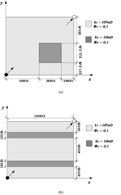
To illustrate the performance of the methodology proposed in Sections 3 and 4 we present the re-sults of tracer injection simulations in a quarter of a repeated five-spot pattern in two dimensions consisting of a square domain (unit thickness) with sideL=1000ft. The injector well is located at the lower-left corner (x=y=0) and the producer well at the upper-right corner (x=y=L). The coefficients have been chosen asαmol=0.0,αl=1.0ft,αt=0.0ftand the porosityφ=0.1. The tracer slug is 0.25% of the porous volume. These data were taken from [21].
In all simulations we use uniform meshes of 80×80 bilinear quadrilateral elements to ap-proximate concentration as well as velocity and pressure. Equal order interpolation functions (m=l=r=s=1) are employed to all variables. Discontinuous Lagrangian interpolation to the SDHM method and continuous Lagrangian interpolation to the Galerkin method and post-processing technique are used. The post-post-processing stabilization parameter is fixed asτ=1.0 and the stabilization parameter associated with the Lagrange multiplier in SDHM is β0=0. The semi-analytical methodology parameters are ˆc=1.0,Vtr=1000ft2,qt=200ft2/day and Nsl=399.
In order to compare the differents approaches described in Section 3, we take into account three scenarios: Case 1, Case 2 and Case 3. In Case 1 the porous medium is homogeneous with the permeability constant, K=1000 mDand the other scenarios consider heterogeneous porous media with subregions having different permeability values (Figure 1).
5.1 Homogeneous Porous Medium
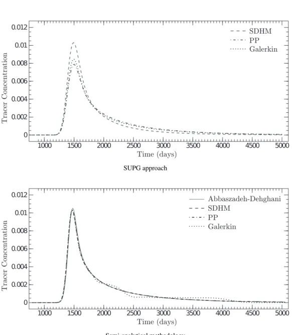
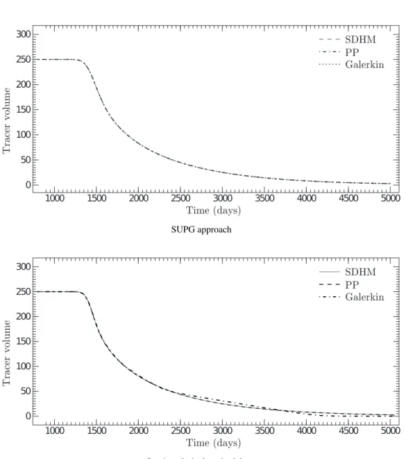
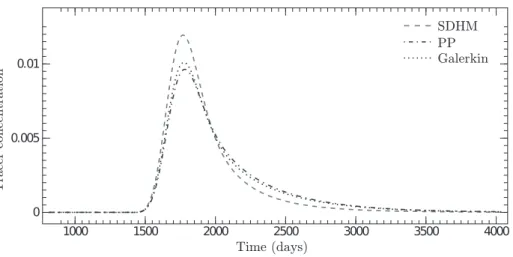
Figure 2 exhibits comparisons between the results of the SUPG approach and the semi-analytical methodology for the concentration with velocity approximations obtained by the SDHM formu-lation, the post-processing technique (PP) and the Galerkin method. For both approximations we see that the SDHM method has the closest profile to the analytical solution obtained by Abbaszadeh-Dehghani [1] (peak at 0.01) as showed in Figure 2-(b). The conservative property of the SDHM method is illustrated in Figure 3. Therefore, we can conclude that the SDHM for-mulation is the more stable and provides accurate results in all approaches considered here for the transport equation.
5.2 Heterogeneous Porous Media
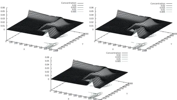
In this subsection, we consider two problems defined in the heterogeneous domains plotted in Figure 1 (Case 2 and Case 3). Figures 5 and 6 show the tracer concentration maps att=1000 days when we use the SUPG approach combined with the Galerkin method, the post-processing technique and the SDHM method to∆t=5 days. Similar transport behaviours are observed for all velocity approximations.
(a)
(b)
SUPG approach
Semi-analytical methodology
SUPG approach
Semi-analytical methodology
THE INFLUENCE OF VELOCITY FIELD APPR O XIMA TIONS IN TRA CER INJECTION PR OCESSES
500 1000 1500 2000 2500 3000 3500 4000 4500 5000
Time (d ays)
0 0.002 0.004 0.006 Tr ac e r co n ce n tr at io
1000 1050 1100 1150 1200 1250 1300 1350 1400 1450 1500 1550 1600
Time (d ays)
0 0.001 0.001 Tr ac e r co n ce n tr at io
500 1000 1500 2000 2500 3000 3500 4000 4500 5000
Time (d ays)
0 0.002 0.004 0.006 0.008 0.01 Tr ac e r co n ce n tr at io n Pe =100 Pe =50 Pe =25 Pe =12. 5
1000 1050 1100 1150 1200 1250 1300 1350 1400 1450 1500 1550 1600
Time (d ays)
0 0.001 0.001 0.002 0.002 Tr ac e r co n ce n tr at io n Pe =100 Pe =50 Pe =25 Pe =12. 5
Figure 4: Case 1 - Time history of the tracer concentration (left) and a zoom in the spurious oscillations region (right). The P´eclet influence study. Galerkin method, post-processing technique and the SDHM method (from top to bottom).
Figure 5: Case 2- Tracer concentration maps. (a) Galerkin method, (b) post-processing technique and (c) the SDHM method.
The time history of the tracer concentration in the producer well for Case 2 and Case 3 using the SUPG approach are showed in Figures 7 and 8 for the concentration with velocity approximations obtained by the SDHM formulation, the post-processing technique (PP) and the Galerkin method. Figure 7 exhibits two concentration peaks due to the influence of the lower permeability region, which act like a barrier to the flow. The SDHM formulation produces the highest peak according to the physical expected behavior. Note that the tracer concentration reaches the producer well and, the peak concentration is achieved, in an earlier time compared with that observed in Case 1 (see Figure 2). This is due to the fact that there are preferential flow paths where the velocity flow is increased as a result of the presence of a subregion of lower permeability.
Figure 7: Case 2 - Time history of the tracer concentration to different velocity field approximations.
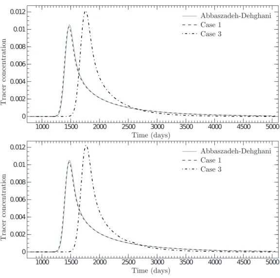
Next in Figure 8 we observe a similar behavior to the homogeneous scenario (Case 1) but with higher concentration values. This can be better understand in Case 1 and Case 3 results plot in Figure 9, where we compare the time history of the tracer concentration obtained by the semi-analytical solution combined with the post-procesing technique and the SDHM formulation. The subregions with differents permeabilities have the same domain width. Therefore, they act as a delay to the flow. Thus, the concentration reaches the producer well later than the Case 1.
SUPG approach
Semi-analytical methodology
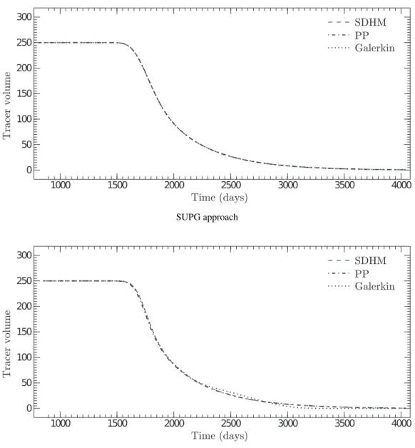
Figure 10: Case 3 - Tracer volume for the tracer concentration. Comparison among the velocity field approximations: (a) and (b) SDHM, Post-Processing (PP) and Galerkin.
6 CONCLUSION
for the concentration. This combination is able to capture the expected discontinuity proper-ties of the solution and, consequently, a proper physical solution. The numerical experiments performed, illustrated the flexibility and robustness of this formulation.
RESUMO. Embora a concentrac¸˜ao seja a vari´avel mais importante nos processos de injec¸˜ao de trac¸adores, uma eficiente e precisa aproximac¸˜ao do campo de velocidades ´e cru-cial para obter um bom comportamento f´ısico para o problema. Neste artigo, analisamos o m´etodo misto dual h´ıbrido estabilizado (SDHM) para resolver o sistema de Darcy nas vari´aveis de velocidade e de press˜ao a partir da equac¸˜ao de conservac¸˜ao de massa e da lei de Darcy. Esta abordagem ´e localmente conservativa, livre de comprometimento entre os espac¸os de aproximac¸˜ao de elementos finitos e capaz de lidar com meios heterogˆeneos com propriedades descont´ınuas. A concentrac¸˜ao do trac¸ador ´e resolvida atrav´es de uma combinac¸˜ao do m´etodoStreamline Upwind Petrov-Galeklin (SUPG) no espac¸o com um m´etodo de diferenc¸as finitas impl´ıcita no tempo. Tamb´em empregamos uma abordagem semi-anal´ıtica (soluc¸˜ao anal´ıtica de Abbaszadeh-Dehghani) para integrar a equac¸˜ao de transporte. Um estudo comparativo num´erico utilizando a formulac¸˜ao de SDHM, o m´etodo de Galerkin e uma t´ecnica de p´os-processamento para calcular o campo de velocidade em combinac¸˜ao com essas metodologias de aproximac¸˜ao da concentrac¸˜ao s˜ao apresentados. Em todas as comparac¸˜oes, a formulac¸˜ao SDHM aparece como a mais eficiente, precisa e quase sem oscilac¸˜oes esp´urias.
Palavras-chave: Deslocamentos misc´ıveis, M´etodos hibridizados, Simulac¸˜oes de reservat´orios de ´oleos
REFERENCES
[1] M. Abbaszadeh-Dehghani & W.E. Brigham. Technical report.Stanford University, (1982).
[2] D.N. Arnold & F. Brezzi. Mixed and nonconforming finite element methods: implementation, post-processing and error estimates.RAIRO MMAN,19(7)(1985), 7–32.
[3] D.N. Arnold, F. Brezzi, B. Cockburn & L.D. Marini. Unified analysis of discontinuous Galerkin methods for elliptic problems.SIAM Journal on Numerical Analysis,39(5)(2002), 1749–1779.
[4] G. Barrenechea, L.P. Franca & F. Valentin. A Petrov-Galerkin enriched method: A mass conserva-tive finite element method for the Darcy equation. Computer Methods in Applied Mechanics and Engineering,196(2007), 2449–2464.
[5] T.P. Barrios, J.M. Casc´on & M. Gonz´alez. A posteriori error analysis of an augmented mixed finite element method for Darcy flow. Computer Methods in Applied Mechanics and Engineering, 283 (2015), 909–922.
[6] F. Brezzi. On the existence, uniqueness and approximation of saddle point problems arising from Lagrange multipliers.Analyse num´erique/Numerical Analysis (RAIRO),8(R-2)(1974), 129–151.
[8] F. Brezzi & M. Fortin. “Mixed and Hybrid Finite Element Methods”. Springer-Verlag (1991).
[9] A.N. Brooks & T.J.R. Hughes. Streamline Upwind Petrov-Galerkin Formulations for Convection-Dominated flows with Particular emphasis on the Incompressible Navier-Stokes Equations.Comput. Methods Appl. Mech. Engrg.,32(1982), 199–259.
[10] M.R. Correa & A.F.D. Loula. Stabilized velocity post-processings for Darcy flow in heterogenous porous media.Communications in Numerical Methods in Engineering,23(2007), 461–489.
[11] M.R. Correa & A.F.D. Loula. Unconditionally stable mixed finite element methods for Darcy flow.
Computer Methods in Applied Mechanics and Engineering,197(2008), 1525–1540.
[12] I.H.A. da Igreja. “M´etodos de elementos finitos h´ıbridos estabilizados para escoamentos de Stokes, Darcy e Stokes-Darcy acoplados”. Ph.D. thesis, Laborat´orio Nacional de Computac¸˜ao Cient´ıfica, Petr´opolis, Brasil (2015). URLhttp://tede.lncc.br/handle/tede/225.
[13] B.L. Darlow, R.E. Ewing & M.F. Wheeler. Mixed finite element method for miscible displacement problems in porous media.SPE Journal, (1984), 391–398.
[14] A. Datta-Gupta & M.J. King. A semianalytic approach to tracer flow modeling in heterogeneous permeable media.Advances in Water Resources,18(1)(1995), 9–24.
[15] J.J. Douglas, R.E. Ewing & M.F. Wheeler. The approximation of the pressure by a Mixed-Method in the simulation of miscible displacement.R.A.I.R.O. Analyse Numerique,17(1983), 17–33.
[16] J.J. Douglas & J. Wang. An absolutely stabilized finite element method for the Stokes problem.Math. Comput.,52(186)(1989), 495–508.
[17] R.E. Ewing, J. Wang & Y. Yang. A stabilized discontinuous finite element method for elliptic problems.Numerical Linear Algebra with Applications,10(2003), 83–104.
[18] I. Harari. Stability of semidiscrete formulations for parabolic problems at small time steps.Comput. Methods Appl. Mech. Engrg.,193(2004), 1491–1516.
[19] A.F.D. Loula, F.A. Rochinha & M.A. Murad. Higher-order gradient post-processings for second-order elliptic problems.Computer Methods in Applied Mechanics and Engineering,128(1995), 361–381.
[20] S.M.C. Malta & A.F.D. Loula. Numerical analysis of finite element method for miscible dis-placements in porous media. Numerical Methods in Partial Differential Equations, 14 (1998), 519–548.
[21] S.M.C. Malta, A.F.D. Loula & E.L.M. Garcia. Numerical analysis of a stabilized finite element method for tracer injection simulations.Comput. Methods Appl. Mech. Engrg.,187(2000), 119–136.
[22] A. Masud & T.J.R. Hughes. A stabilized finite element method for Darcy flow.Computer. Methods Appl. Mech. Engrg,191(2002), 4341–4370.
[24] Y.R. N´u˜nez, C.O. Faria, A.F.D. Loula & S.M.C. Malta. A mixed-hybrid finite element method applied to tracer injection processes. International Journal of Modeling and Simulation for the Petroleum Industry,6(1)(2012), 51–59.
[25] Y.R. N´u˜nez, C.O. Faria, A.F.D. Loula & S.M.C. Malta. A hybrid finite element method applied to miscible displacements in heterogeneous porous media. Rev. Int. de M´etodos Num´er. C´alc. Dise˜no Ing.,33(1-2)(2017), 45–51.
[26] D.W. Peaceman. “Fundamental of Numerical Reservoir Simulation”. Elsevier, Amsterdam (1977).
[27] P.A. Raviart & J.M. Thomas. A Mixed Finite Element Method for Second Order Elliptic Problems. In I. Galligani & E. Magenes (editors), “Lecture Notes in Math”, volume 606. New York, Springer-Verlag (1977).