S
TOCHASTIC
M
ODEL FOR
S
IMULATING
M
AIZE
Y
IELD
E. R. Detomini, D. Dourado Neto, J. A. Frizzone, A. Doherty, H. Meinke,
K. Reichardt, C. T. S. Dias, M. G. Figueiredo
ABSTRACT. Maize is one of the most important crops in the world. The products generated from this crop are largely used in the starch industry, the animal and human nutrition sector, and biomass energy production and refineries. For these reasons, there is much interest in figuring the potential grain yield of maize genotypes in relation to the environment in which they will be grown, as the productivity directly affects agribusiness or farm profitability. Questions like these can be investigated with ecophysiological crop models, which can be organized according to different philosophies and structures. The main objective of this work is to conceptualize a stochastic model for predicting maize grain yield and productivity under different conditions of water supply while considering the uncertainties of daily climate data. Therefore, one focus is to explain the model construction in detail, and the other is to present some results in light of the philosophy adopted. A deterministic model was built as the basis for the stochastic model. The former performed well in terms of the curve shape of the above-ground dry matter over time as well as the grain yield under full and moderate water deficit conditions. Through the use of a triangular distribution for the harvest index and a bivariate normal distribution of the averaged daily solar radiation and air temperature, the stochastic model satisfactorily simulated grain productivity, i.e., it was found that 10,604 kg ha-1 is the most likely grain productivity, very similar to the productivity simulated by the deterministic model and for the real conditions based on a field experiment.
Keywords. Bivariate normal distribution, Corn, Crop modeling, Depleted productivity, Grain productivity, Triangular distribution.
he advent of crop models implemented on computers can be traced back to groundbreaking work in the 1950s, such as the study by Monsi and Saeki (1953) on light interception and de Wit’s (1958) classic “Transpiration and Crop Yields” that also draws on some of Penman’s early work (Penman, 1948). These and similar publications constructed the framework for the emerging formalism of system analysis (Zadoks and Rabbinge, 1985). Phrasing physiological processes in mathematical terms and collating them to meteorological variables led to today’s proliferation of computer simulation models that have been developed and used in agriculture.
Simulation models of agricultural plants, crops, and cropping systems are becoming commonplace. Traditionally, they have been used as knowledge depositories by scientists to describe an area of interest. Once available, interest quickly shifted from curiosity about the underlying principles to the use of models either in a predictive capacity (e.g., to develop scenarios or to support decisions) or in an explanatory capacity to investigate interactions between processes studied in an isolated manner. This manner of studying models initiated a debate about the appropriateness of mathematically describing biological relationships and the level of details needed to achieve a “good” model. Defining this goodness, by clearly stating the objectives of every modeling endeavor, could make much of that debate redundant (Meinke, 1996).
Arguments about the right way to build crop models have largely concentrated on the level of empiricism acceptable when representing such sequences mathematically. Passioura (1996) asserted that the purpose of scientific models is to improve our understanding of physiology and environmental interactions, while engineering models utilize robust, empirical relationships to obtain results. This separation would constitute a traditional reductionist paradigm because it would reinforce the disassociation of scientific and engineering modeling rather than allow for a synthesis of the different approaches. Rather than separating engineering from science and alienating many professionals in the process, it might be more useful to view this differentiation as the pragmatic end of a continuous quest for knowledge and a solution to the problems. Used constructively, this polarity should advance future model developments (Meinke, 1996). Submitted for review in August 2009 as manuscript number BE 8178;
approved for publication by the Biological Engineering Division of ASABE in May 2012.
The authors are Euro Roberto Detomini, PhD, Department of Biosystems Engineering, University of São Paulo, Brazil; Durval Dourado Neto, Full Professor, Department of Crop Sciences, University of São Paulo, Brazil; José Antonio Frizzone, Full Professor, Department of Biosystems Engineering, University of São Paulo, Brazil; Alastair Doherty, Computer Programmer, Department of Primary Industries and Fisheries, Toowoomba, Queensland, Australia; Holger Meinke, Adjunct Professor, Department of Land and Water, Wageningen Rural University, Wageningen, The Netherlands; Klaus Reichardt, Soil Physics Researcher, Centre of Nuclear Energy in Agriculture, University of São Paulo, Brazil; Carlos Tadeu dos Santos Dias, Full Professor, Department of Exact Sciences, University of São Paulo, Brazil; and Margarida Garcia de Figueiredo, Professor Adjunto, Agribusiness and Regional Development Postgraduate Program, Federal University of Mato Grosso, Brazil. Corresponding author: Euro Roberto Detomini, ESALQ/USP, Departamento de Engenharia de Biossistemas, Av. Pádua Dias 11, Piracicaba - SP, CEP 13418-900, Brazil; phone:+55-19-3429-4217; e-mail: erdetomini@hotmail.com.
Thus, models are simplified representations of a system that is a part of the real world and contains related compo nents inside predefined boundaries. This system can be af fected by the surroundings, but the surroundings cannot af fect it significantly. The definition of scale is very important to ensure that the conclusions of a system will of ten be based on the performance of the low hierarchy com ponents. The main roles of models, in our understanding, are to: (1) organize information; (2) highlight gaps in the various research areas of knowledge; (3) visualize a robust idea about the potentialities, limitations, or eventually magnitudes of a given variable of interest; and (4) simulate impossible and difficult scenarios (e.g., CO2 injection on
earth, insect biology studies). Moreover, the existence of a coincidence does not necessarily imply a cause effect rela tionship.
The applicability of crop models emerges when one needs to optimize the use of resources such as land and wa ter under given boundary conditions. For example, if an economist intends to calculate the highest possible profita bility under certain resource constraints (i.e., land and wa ter) over the course of an agricultural project, the analysis regarding how much water and land area could be available for cropping during a couple of years will depend on re fined and well established crop models. This analysis cer tainly justifies modeling research efforts meant to improve simulation outputs. It is convenient, for instance, to classify models only as deterministic and stochastic, regardless of other non straightforward distinctions. Although determin istic models can output a solution through simple mathe matical implementation, they are limited because they pro vide only a single outcome. In contrast, stochastic models, which use statistical methods or stochastic components, provide a range of results, with each result associated with its corresponding probability of occurrence.
Maize is one of the most important crops in the world. The products generated from this crop are largely used in the starch industry, the animal and human nutrition sector, and biomass energy production and refineries. For these reasons, there is frequently a significant interest in knowing the potential grain yield of maize genotypes in relation to the environment in which they will be subjected for crop ping, as productivity directly affects agribusiness or farm profitability. The main objective of this work is to concep tualize a stochastic model for predicting maize grain yield and productivity under different conditions of water supply while considering the uncertainties of daily climate data. A deterministic model and some outputs are also analyzed to evaluate the time course of the above ground dry matter growth of maize.
M
ATERIALS A D
M
ETHODS
MODEL DESCRIPTIO A D A BRIEF PARAMETERIZATIO
The proposed model includes concepts from both gener ic (i.e., the family of Dutch models) and maize specific (i.e., CERES Maize; Jones and Kiniry, 1986) approaches.
Our maize model includes assimilation processes and de pends on few empirical input parameters; it does not pre dict any crop phenology except the physiological maturity point as a function of thermal time. Dobermann et al. (2003) provided a good comparison between each family of models by pointing out a number of advantages and disad vantages of each family.
From dimensional analysis, Detomini (2008) derived the following mechanistic equation for estimating the potential above ground dry matter (DM) on a daily basis:
0.1498
IWpa
=
⋅
GP
⋅λ ⋅
RUE
(1)
where Wpa is the potential above ground dry matter (kg DM ha1 d1) estimated for a given day, GP is the gross photosynthesis rate (kg CH2O ha1 d1), λI is the fraction
of solar radiation intercepted by the canopy, and RUE is the radiation use efficiency (g above ground dry matter MJ1 intercepted photosynthetically active radiation).
The GP function was also deducted by collating Clapeyron’s law with dimensional analysis according to Detomini (2008):
36.5854
273
GAR LAI H P GP
T
⋅ ⋅ ⋅ ⋅
=
+ (2)
where GAR is the gross assimilation rate ( L CO2 cm2
leaf area h1), LAI is the leaf area index, H is the day length (h d1), P is the atmospheric pressure (atm) that re lies on altitude (Alt, m), and T is the daily average air temperature (°C). Clapeyron’s law is generally used to convert the volume of a given substance into its corre sponding mass, leading to a justification of GAR units in a volume basis. Substituting equation 2 into equation 1 yields:
5.48
273 I
GAR LAI H P
Wpa RUE
T
⋅ ⋅ ⋅
= λ
+ (3)
Bouger Lambert’s law states that photosynthetically ac tive radiation transmitted (PARt, MJ m2 d1) vertically
through a canopy can be derived from Beer’s law (Monsi and Saeki, 1953):
(
)
0 k LAI
t
PAR =PAR e− ⋅
(4)
where PAR0 refers to the incident photosynthetically ac
tive radiation flow (MJ m2 d1) on top of the canopy, and k is the light extinction coefficient. The ratio PARt/PAR0
defines transmittance (τ) so that the complementary frac tion (1 – τ) defines the intercepted fraction (λI). For prac
tical purposes, λI could also be understood as a canopy
covering fraction if canopy leaves are randomly oriented and spread (Loomis and Connor, 1992, p. 274).
light extinction coefficient rapidly decreases as LAI values increase during the initial stages of crop development, but it is likely to assume a constant value if the canopy closes fast (i.e., under irrigated field conditions). Because of this, the in itial variations of k can be neglected for crop model purposes in non limiting conditions of water (Meinke, 1996).
It is important to highlight that equation 3 explains the daily above ground dry matter as a function of plant varia bles, such as RUE, k (implicit, see eq. 4), GAR, and LAI, and as a function of seasonal and climate variables, such as day length (H), atmospheric pressure (P), temperature (T), and absorbable radiation flow. This latter variable can be explicitly stated by expressing GAR (eq. 7) as a function of equation 5, which relies on both air temperature and solar radiation flow (implicit, see eq. 6). By analyzing data from the graphs shown by Heemst (1986) for C4 plants, Detomini (2008) presented an empirical generic function for describing the potential gross assimilation rate (GARp,
L CO2 cm2 leaf area h1) under controlled conditions:
( )
( )
( )
2 3
0 1 2 3 4
2
2 3
5 6 7 8 9
ln
1 ln ln
p
ab ab ab
ab ab ab
GAR
A A R A R A R A T
A R A R A R A T A T
=
+ + + +
+ + + + +
(5)
where T is the air temperature (0 < T < 40°C), and Rab is
the absorbable photosynthetically active radiation flow (0 < Rab < 0.35 cal cm2 leaf area min1). The empirical,
non user defined parameters are: A0 = 1.566792, A1 =
53515909, A2 = 221.805971, A3 = 310.191491, A4 =
0.491961, A5 = 0.190506, A6 = 0.373910, A7 =
0.088166, A8 = 0.554728, and A9 = 0.080398.
In fact, the absorbable photosynthetically active radia tion flow was derived from a dimensional analysis by Detomini (2008) as a function of solar radiation flow (Rg, MJ m2 d1) and day length (H, h d1) with some corrections:
(
)
0.3987 1
ab PAR ab r
Rg R
H
= λ λ − λ
(6)
According to Sinclair and Muchow (1999), representa tive values for λPAR and λab would be 0.5 (MJ
photosynthetically active radiation MJ1 incident solar radi ation) and 0.85 (MJ absorbable radiation MJ1 photosynthetically active radiation), respectively. Oguntunde and van de Giesen (2004) suggested a value of λr = 0.23 (MJ soil plant reflected radiation MJ1 incident
solar radiation) for maize crop albedo.
GARp is corrected by cloudiness effects according to:
(
1)
4ub Adc 4ub p
GAR=F R + −F GAR
(7)
where RAdc, specific to genotype, is the relationship be
tween gross assimilation rates under a clear sky and gross assimilation rates under an overcast sky; and F4ub, specif
ic to environment, is a cloudiness factor responsible for correcting the theoretical potential gross assimilation rate. The magnitude of the former was simulated to be around 0.2626 (Detomini, 2008), whereas the latter might be di rectly obtained if insolation data are available or, if not,
estimated by implying that radiation flow during strongly overcast days accounts for 20% of the flow on very clear days, according to:
(
)
1.25 1
4ub
AP AP T
Rg F
a b R
= −
+
(8)
where aAP and bAP are the Angström Prescott coefficients,
and RT is the estimated radiation incident on top of the
atmosphere once the Earth’s eccentricity (DRST2) and sunset hour angle (Ahn, degrees) are calculated:
(
)
2
37.6 sin sin 180 180
cos cos sin 180 180 T
R DRST Ahn
Ahn
π π
= ⋅ Φ ζ
π π
+ Φ ζ
(9)
2 2
1 0.033 cos
365
DRST = + DOY π
(10)
24
H Ahn=π
(11)
Note that equation 7 turns the generalized equation (eq. 5) into a specific condition by collating information from the plant (RAdc), the climate (Rg), and the local (aAP, bAP,
and RT) conditions for a given day of the year (DOY). The
resulting angle between the imaginary plane of the equator and the imaginary line that links earth to the sun defines the solar declination (ζ, degrees) and relies on DOY:
(
)
2
23.45sin 80
365 DOY π
ζ = −
(12)
Thus, the length of a given day might be obtained as:
24
arccos tan tan
180 180
H = − ζ π −Φ π
π (13)
where Φ refers to the latitude (decimal values) of the place of interest. Negative values of Φ are conventionally set for locations in the southern hemisphere.
Because plant populations depend on both plant density of sowing (Dsow, plants m1) and spacing (Se, m), these
measurements are required for defining the leaf area index (LAI) in addition to the leaf area (LA, cm2 plant1). At a farm level view:
4
10 sow
e D
LAI LA
S − =
(14)
extrapolating this model for the whole plant because it re quires empirical linear fittings for predicting the largest ar ea and leaf position, in addition to the eventual leaf number. We suggest using a closed empirical Gauss model, which is somewhat similar to the mechanistic model presented by Yang and Alley (2005). The functional form of our Gauss model is:
( )
2 2 3 0.5
1e
Dr
LA Dr
−γ
− γ
= γ
(15)
where Dr is the relative crop development, and γ1, γ2, and
γ3 are the empirical parameters.
The first parameter (γ1) of equation 15 is biologically
meaningful because it represents the maximum value of the entire plant leaf area (LAmax), equal to 8654.91 cm2 in a
model where Dr = γ2 = 0.5758 (Detomini, 2008). The
meaning of the third parameter (γ3) is not well established,
although it approximately a quarter of the entire Dr (γ3 =
0.2473). Instead of considering time for crop development duration, this parameter was considered on a dimensionless basis (i.e., Dr) to allow better generalization for future comparisons with data obtained from other studies and ex periments.
The relative crop development defines the cumulative thermal time (CTTj, °C d) on the jth day after emergence in
relation to the cumulative thermal time at a physiological maturity point (CTTmpp, °C d), consistent with the following
approach:
j j
mpp
CTT Dr
CTT
=
(16) The value of CTTmpp was found as 1392.82°C d from
field experimental data (Detomini et al., 2008). However, the variable is user defined in the model and varies accord ing to maize genotype. The CTT is the sum of single daily thermal times (TTj, °C):
1
n
j j
j
CTT TT
=
=
∑
(17)
If the relative development rate is well represented by a non linear function but has a linear relationship with TT, this variable can also be described by a non linear function. After reviewing “degree days” concepts, Bonhomme (2000) explained the limitations of traditional degree day calculation methods and suggested a beta function to calcu late TT, with upper (TDmax, °C), lower (TDmin, °C), and op
timal (TDop, °C) temperatures for development. First pro
posed by Yin et al. (1995), the beta function is assumed as the best option to calculate thermal times because it is based on relatively flexible mathematical laws and has few parameters, all physically and biologically meaningful, ac cording to:
min max
max min
max
max min
op op
TD TD
TD TD
op op
TT
TD T T TD
TT
TD TD TD TD
− −
=
− −
− −
(18)
Assuming user defined values of TTmax, TDmax, TDop,
and TDmin equal to 25, 44, 35, and 0, respectively, the func
tion that particularly describes thermal time as a function of air temperature will only depend on daily air temperature (T, °C), for example:
3.89
0.0793(44 )
TT= −T T
(19)
A helpful approach to establishing a relationship be tween water and yield productivity was proposed by Doorenbos and Kassam (1979):
1
1 1
n
i i
Wa WUa
ky
W = WU
= − −
∏
(20)
The ky values for most crops are derived under the as sumption that the relationship between relative yield (Wa/W) and relative water use (WUa/WU) is linear and is valid for water deficits up to about 50%, or (1 – WUa/WU) = 0.5. The values of ky are based on an analysis of experi mental field data covering a wide range of growing condi tions. The experimental results used represent high producing crop varieties, well adapted to the growing envi ronment and grown under a high level of crop management. The ratio WUa/WU may either occur continuously throughout the entire growth period of the crop, or it may occur during any one of the individual growth periods (i.e., i = 1, 2, …, n). Analysis of the available experimental field data in terms of the more precisely defined stress day and drought indices proved difficult. On the other hand, if a simulation process is modeled on a one day scale, the orig inal production model of Doorenbos and Kassam (1979) collapses because the day to day multiplication of a deci mal factor would quickly deplete the production. To solve this problem, our model assumes a continuous and equally distributed day to day water deficit to calculate the produc tivity depletion, as will be shown later, so that a value of 1.25 might be adopted for maize hybrids in this situation. Thus:
1 Wpad 1.25 1 ETa
Wpa ET
− = −
(21)
where Wpad is the depleted, above ground dry matter productivity rate (kg ha1 d1), ETa is the actual evapotran spiration (mm d1), and ET is the potential evapotranspira tion (mm d1).
opposite (i.e., 1 – ETa/ET) would be the level of stress. If Wpad is explicit and Sw is inserted into equation 21:
(
)
1 1.25 1
Wpad =Wpa − −Sw
(22)
The term inside the brackets is, therefore, a depletion factor (Fd; kg potential above ground dry matter productiv ity rate kg1 depleted above ground dry matter productivity rate). By inserting equation 3 into equation 22, it is possible to find a simple model to predict depleted above ground dry matter productivity rates on a daily basis as:
(
)
5.48 1 1.25 1
273 I
Wpad
GAR LAI H P
RUE Sw
T =
⋅ ⋅ ⋅
λ − −
+ (23)
In agreement with the approach of Verdoodt et al. (2004), the summation of daily dry matter (eq. 23) until reaching the economically useful stage of a crop, which in this model is the maturity point, results in the final cumu lated above ground dry matter productivity that should ac count for harvest index (HI; kg grain kg1 depleted above ground dry matter) in the calculation for the grain produc tivity simulation (Wg; kg grain ha1):
0
n
j j
Wg HI Wpad
=
=
∑
(24)
According to equation 24, there is no plant weight loss. This weight stability might be justified because the daily calculations of Wpa already account for the efficiency of radiation use (RUE), and the senescing losses are accounted for in the LAI equation. Equation 24 is the final determinis tic model used to predict maize grain productivity (on a dry
basis) under specific limited and non limited water supply, climate, population, site, and time conditions. The stochasticity can be implemented simultaneously through climate variables (i.e., temperature and solar radiation) and the harvest index.
The flowchart in figure 1 summarizes the main concept of the model. Some equations are implied in the flow and are not presented. For example, it is observed that the vari able T is used in equation 16, but it is important to mention that T is first used in equation 19, which leads to equation 17 and then to equation 16. The input variables Dsow and Se
(both related to population), DOY (related to the date of sowing), Φ and Alt (both related to place), and Sw (related to water management) are all user defined variables, as are RUE, k, λPAR, λab, λr, and RAdc (all related to light plant rela
tions). The user defined variable HI is considered in a sto chastic manner through a triangular distribution, whereas T and Rg can be likewise considered through a triangular (if there is no data series) or bivariate normal distribution.
An initial parameterization was considered as: RUE = 3.52, k = 0.4257, HI (mode = 0.4, maximum = 0.43, mini mum = 0.38), and LA(Dr) according to equation 15. We used equation 5 for gross assimilation rate and equation 19 for thermal time. We also used user defined values for lati tude ( 22.425), Angström Prescott coefficients (aAP = 0.25;
bAP = 0.5), plant population (66,666 plants ha1), row spac
ing (0.9 m), and date of sowing (24 November), in addition to the experimental weather data. Above ground dry matter productivity rates (Wpa, kg ha1 d1), cumulated above ground dry matter (W, kg ha1), and maize grain productivi ty (Wg, kg ha1) were calculated using equations 23 and 24 through a deterministic simulation. Additionally, RAdc =
0.26 was iteratively adjusted.
A sensitivity analysis was run in a simple manner by an
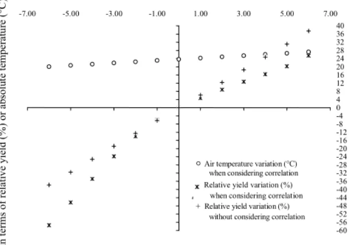
alyzing how much the grain yield (in percentage) would be increased or reduced for each added or subtracted unit of MJ m2 d1 of solar radiation, considering a correlation be tween solar radiation and temperature, in relation to the yield observed from climate data of the field experiment carried out by Detomini (2008). Prior to these analyses, we also performed a sensitivity analysis for the empirical and fitted equation 5, which represents the variation of potential gross assimilation rate as a function of solar radiation for many levels of air temperature (see fig. 2).
STOCHASTIC PROCEDURE USI G EITHER BIVARIATE ORMAL DISTRIBUTIO OR TRIA GULAR DISTRIBUTIO
Considering a variable such as maize grain yield, the model is deterministic because it will reproduce the exact same outputs for a given set of input variables. For situa tions where externalities or uncertainties can be neglected because they have little effect on the outputs, deterministic models are reasonably acceptable in some situations (e.g., irrigation design, mixture of chemicals under controlled conditions, or fertilizer recommendation for “homogene ous” soils). On the other hand, variability might be deter minant on the final output (e.g., on the same day of the year in a given place, the average air temperatures might be around 10°C, 20°C, or even 30°C, highly affecting the final plant growth rate). A stochastic procedure would consider this variability by releasing too many outputs instead of on ly one, with each one related to its corresponding probabil ity of occurrence.
Air temperature, for example, can reveal infinite possi bilities of occurrence, even though some frequency around a given value will most likely occur. This frequency can be low or high for extreme or expected values. A group of in finite possibilities associated with their corresponding val ues can be eventually expressed by a probability density function, and its integration gives the probability function if all function properties are confirmed. A Monte Carlo meth od consists of inverting the resulting integration and explic itly declaring the variable, when possible, remaining only using known values of the probabilities for the simulation initiation. In fact, pseudo random numbers are the starting point of a Monte Carlo simulation. Matsumoto and Nishi mura (1988) developed the Mersenne Twister algorithm that is used in most recognized statistical packages to gen erate the starting points. The simulation error (ε) is mini mized inversely according to the iteration number (4i), yet it also relies on the deviation (σ) of a dataset:
3 4i
σ ε =
(25)
Within the various existing probability distributions, ei ther discrete or continuous, the normal distribution is the most important from the agronomic knowledge viewpoint, not only because many processes are well explained by it but also because it is a sort of “outer limit” of most of the distributions. Ideally, a distribution is adopted for a dataset if it describes the distribution properly, which can be veri
fied by tests like Kolmogorov Smirnov. Because a variable distribution is an average, the central limit theorem states that if a sample is too large (n → ∞), variance is then min imized [(σ2/n) → 0] by trending to zero, leading a variable to approximately follow a normal distribution [~4 ( , σ2
/n)] (i.e., strongly bell shaped) even for non normal pop ulations. Additionally, the normal distribution fits many sample probability distributions very well. A simple starting point for simulating two variables that presumably follow normal distributions, based on a high 4i, is to use the Box Muller transformation to obtain auxiliary variables 1 and 2 (41 and 42), which depend on a previous generation of
pseudo random numbers U1 and U2 that are independent
from each other and are uniformly distributed according to (Box and Muller, 1958, p. 610):
( )
0.5(
)
1 2 ln 1 cos 2 2
4 = − U πU
(26)
( )
0.5(
)
2 2 ln 1 sin 2 2
4 = − U πU
(27)
For example, if one intends to generate solar radiation and air temperature for each day of the year, the first step would be to generate two pseudo random values (U1 and
U2, both between 0 and 1) and to replicate this step 4i
times (i.e., 4i = 10,000), i.e., there will be 10,000 values for both U1 (1U1, 2U1, …, 10000U1) and U2 (1U2, 2U2, …, 10000
U2) for each day. As a result, variables 1
41,
2
41, …, 10000
41 and also 1
42,
2
42, …, 10000
42 will exist. As solar ra
diation drives practically all processes on Earth, the value of this variable is hierarchically generated first. By adapt ing the procedure provided by Hogg and Craig (1978), the ith value of solar radiation (iRg) for whatever day for the ith computer generated auxiliary 1 variable (i41) is:
1
i i
Rg Rg
Rg= + σ 4
(28)
where Rg and σRg are calculated (from the dataset) from
the average and standard deviation of solar radiation for one day. Note that equation 28 is the inversion of the standardized variable Z, where Z ~ 4( Rg, σRg).
The ith value of temperature (iT) can be subsequently simulated for the same day by considering the ith computed auxiliary 2 generated variable (i42), the calculated average
and standard deviation of air temperature ( T and σT, re
spectively) for the same day, the simulated value from equation 28, and Pearson’s product moment coefficient correlation (ρ) existing between the variables Rg and T:
(
) (
2)
0.5 21
i
i i
T
T Rg T
Rg
T
Rg 4
=
σ
+ ρ − + − ρ σ
σ
(29)
the observed values. This validation would allow us to identify the type of simulation that best agrees with the ob servations. Pearson’s correlation coefficient may vary from
1 to 1 and equals zero if variables are independent, where as covariance evaluates how the dependent variables “walk” together independent of sample size (Wonnacott and Wonnacott, 1985, p. 132). If ρ = 0 in equation 29, the T calculation is arranged in an analogous manner to equation 28. The correlation measures the strength and linear direc tion between two quantitative variables. For our samples (Moore, 1995, p. 111):
(
)
(
)
(
)
(
)
1
2 2
1 1
n
i Rg i T
i
n 4
i Rg i T
i i
Rg T
Rg T
=
= =
− −
ρ =
− −
∑
∑
∑
(30)
If there are no climate data, it is necessary to search for information from a specialist to derive the subjective pa rameters of the triangular distribution, which is often used in agribusiness when one wants to subjectively describe a population of a continuous variable. The three key parame ters of the triangular distribution are mode or “most likely” (Mo), maximum (Vmax), and minimum (Vmin). To initiate the
triangular generation through the Monte Carlo method, a critical pseudo random number (Uc) should first be calcu lated according to:
min max min
Mo V Uc
V V
− =
−
(31)
Because of the function discontinuity, three possibilities of function inversion become:
if
X=Mo U=Uc (32)
(
)(
)
0.5min max min min
if
X V U V V Mo V
U Uc
= + − −
< (33)
(
)(
)(
)
0.5max 1 max min min
if
X V U V V V Mo
U Uc
= − − − −
> (34)
Evidence from field experiments shows that as biomass increases, harvest index usually decreases with a non mechanistic explanation. The uncertainty of the harvest in dex and environment relationships also encourages the use of a stochastic procedure during the simulation processes, regardless of assuming empirical relationships or even a single value. Thus, the model assumes a triangular distribu tion for simulating the harvest index by considering user defined values of the mode, maximum, and minimum. In summary, 10,000 pseudo random values are generated to produce the same amount of radiation values and their sub sequently correlated air temperatures, both of which follow normal distributions. This procedure is done for each day (after emergence) of a crop cycle. Ten thousand values of the remnant dependent variables are subsequently calculat
ed, resulting in 10,000 values of grain yield that have to be classified per frequency class in a previously calculated class number. For a given iteration, each calculated value of Wpad (eq. 23) in a given day is summed with the calculated Wpad of the previous day. There is certainly an implied er ror by doing this calculation because two opposite extreme values of radiation may be simulated for two consecutive days, sometimes without any physical sense. Nevertheless, such error is inversely minimized according to the number of iterations (eq. 25). Ten thousand 4i values is a large enough sample size.
The implementation of the stochastic procedures in con ventional worksheets would be possible but tiring and quite confusing in terms of presentation because several outputs would be generated and, consequently, a large number of lines or rows would be required. Therefore, it became con venient to develop a tool in the Visual Studio 2005 (C#) platform to run the model to allow for the best visualization of the results. Some input parameters are mandatory, such as sowing date, latitude and hemisphere, crop spacing, sow ing density, mass of a thousand seeds, Angström Prescott coefficients (the program suggests additional values), and the distribution probability. One should opt for triangular distribution if no climate data are available or for bivariate normal distribution if climate data are available. In the for mer case, a meteorology text file needs to be selected. Set ting the plant parameters is optional. The main output is a histogram of yield probabilities.
To stochastically evaluate the model, a deterministic simulation was first run to check the growth of the above ground dry matter throughout the maize cycle. For specific purposes, we consider the term “calibration” when a known observation of a dependent variable (i.e., maize grain yield) is used to predict an input variable (i.e., RAdc). Thus, the
maize deterministic model was calibrated according to an iterative procedure to find RAdc from Wg = 10,472 kg ha1
(averaged grain yield) observed in the field and assuming constant the other input variables. The input variables RUE, k, and LA(Dr) were chosen according to Detomini et al. (2008); the variables λPAR, λab, λr, aAP, and bAP were adopt
ed according to the literature; RAdc was iteratively adjusted
as a function of grain productivity (Wg = 10,472 kg ha1) found by Detomini (2008); and DOY, Φ, Dsow, and Se were
defined to meet field experiment conditions. Then the sto chastic procedure was run for a different place, e.g., Rock hampton, Australia. The climate variables Rg and T were simulated according to a bivariate normal distribution fed by a climate dataset for this location, and HI was set ac cording to a triangular distribution fed by practical sugges tion based on field experiment results.
(aAP = 0.25; bAP = 0.5), plant population (66,666; row spac
ing = 0.9 m), and date of sowing (24 November). Four situ ations were considered for the stochastic simulation of maize grain: (1) bivariate normal distribution for solar radi ation and air temperature under non water deficit condi tions, (2) triangular distribution for solar radiation and air temperature under non water deficit conditions, (3) reduc tion of plant population by taking Dsow = 5 plants m1 under
non water deficit conditions, and (4) water supply of 75% (Sw = 0.75). The corresponding results are shown in figure 6. In case 2, the mode as well as maximum and minimum values for both variables were based on the Rockhampton radiation and temperature dataset (from 24 November up to 120 days after) as follows: mode of 18 MJ m2 s1 and 21°C, maximum of 32 MJ m2 s1 and 32°C, and minimum of 6 MJ m2 s1 and 15°C.
R
ESULTS A D
D
ISCUSSIO
DETERMI ISTIC SIMULATIO A D SE SITIVITY A ALYSIS
A comparison of the observed (field experiment) vs. simulated (eq. 24) data reveals that the model has a slightly overestimated grain productivity of 1.4%, giving an output, for example, of 10,620 kg ha1. If general data are interpo lated from Heemst (1986) for obtaining RAdc, we would find
values of over 0.3 for this variable. Because specific values of RAdc are seldom explored in the literature for specific
genotypes, this problem would exemplify the importance of models, namely, that they allow for the identification of specific magnitudes of a given variable of interest without needing to experimentally derive them through alternative experimental conditions, which might require additional expenses.
It can be seen from a sensitivity analysis performed for equation 5 that the value of GARp, which depends on solar
radiation, decreases from a maximum of 33°C even if Rab is
rising, according to figure 2, which could also be represent ed by a surface. The graph is presented in a convenient, il lustrative manner. For example, GARp is less responsive to
Rab when under 25°C compared to 39°C, which is a similar
behavior to that found by Lizaso et al. (2005). In spite of being built empirically, the curves satisfactorily represent the process of interest when compared to the curves (simi lar to a rectangular hyperbolic shape, except for low tem perature values) presented by Pachepsky et al. (1996). For physiological reasons, potential gross assimilation rates substantially decrease for overcast days such that it is rec ommended to make the necessary corrections prior to esti mating the actual GAR, following the approaches of Heemst (1986) and Verdoodt et al. (2004). This decrease is the justification for the existing equation 7 to deplete GARp.
We believe one good route to specify GAR for each maize hybrid would be to adjust RAdc and biological meaningful
parameters of the beta function (eq. 18).
Identifying the sensitivity of the maize model yield to solar radiation (the main driving variable) is essential be cause temperature variation is also calculated using correla tion (i.e., eqs. 29 and 30). For example, by adopting climate data from the field experiment of Detomini (2008), figure 3 reveals that each extra unit of MJ m2 d1 added to the daily solar radiation flow values throughout the maize cycle would increase the yield by approximately 4%, which is a variation smaller than that of each unit of MJ m2 d1 sub tracted from each daily value. By correlation, the tempera ture varies linearly by more or less than 0.6°C for each added or subtracted MJ m2 d1, respectively. If the correla tion between solar radiation flow and air temperature is ne glected (i.e., varying the former but keeping the latter con stant), the magnitudes of the simulated yields resulting from added units of radiation become even greater, and yields resulting from subtracted units become even smaller, in comparison to the yields simulated from the aforemen tioned field experiment climate data.
It is worth noting that increasing the amount of radiation by 6 MJ m2 d1 (and ~3.6°C in temperature by correlation) would shorten the time to tasseling by 12 days if the as sumptions of thermal time concepts are valid. A decrease in
Figure 2. Potential gross assimilation rate as a function of absorbable photosynthetically active radiation flows for different air tempera( tures.
Figure 3. Sensitivity analysis for the absolute variation in temperature and relative yield from each unit of MJ m(2 d(1 varied in terms of inci(
dent solar radiation.
0 50 100 150 200 250 300
0 0.1 0.2 0.3
Rab (cal cm2min1)
GA
Rp
(
L
C
O2
c
m
1h 1)
1 ºC 5 ºC 10 ºC 15 ºC 20 ºC 25 ºC 30 ºC 35 ºC 39 ºC
60 56 52 48 44 40 36 32 28 24 20 16 12 8 4 0 4 8 12 16 20 24 28 32 36 40 7.00 5.00 3.00 1.00 1.00 3.00 5.00 7.00
Absolute variation (in MJ m2dia1) in terms of incident solar radiation
Relative yield variation (%) when considering correlation + Relative yield variation (%) without considering correlation
V
ar
ia
ti
o
n
s
in
t
er
m
s
o
f
re
la
ti
v
e
y
ie
ld
(
%
)
o
r
ab
so
lu
te
t
em
p
er
at
u
re
(
°C
)
radiation by the same value would stretch this time to 23 days. In fact, this phenological stage was observed in the field at 55 days after emergence. The proposed model does not release the outcome of tasseling. However, these varia tions in time are realistic because shortening the maize cy cle could eventually lead to a premature definition of the number of leaves, whereas stretching it could provoke ex cessive growth of vegetative components, especially with regard to stalk height, mass, and carbohydrate storage. In the case of increasing radiation, for example, the anticipat ed growth determination could reduce the productivity in a manner contradictory to that identified by sensitivity analy sis unless the hybrid was sown in a non recommended place and season. In a second case, for constant given water and nitrogen conditions, the sink source relationships could be altered to reduce the yield because the competition of assimilates among the different plant tissues would in crease.
The harvest index is another attribute that could be strongly modified with the variation of both climate varia ble magnitudes and maize biological cycle length, resulting in either a reduction or increase in grain yield. However, this sensitivity is difficult to analyze, as the harvest index generally has an inverse relationship with plant growth, which does not necessarily mean that the productivity would be smaller, as observed by Detomini (2008). Addi tionally, it is difficult to study the effects of climate inputs on HI because the variation is not even throughout the cy cle, besides the fact that the main periods (vegetative, flow ering, and grain filling) contribute through different routes to the HI and are different from each other in terms of weather sensitivity.
Quite high values of above ground dry matter productiv ity rates (Wpa) were calculated, which surpassed 600 kg ha
1
d1 during the most exigent stage of the cycle (flowering); yet low values of Wpa were simulated for the initial stages (i.e., before 40 DAE), as expected due to low values of LAI and light interception during theses stages. Loomis and Connor (1992, p. 41) reported rates at a magnitude of 520 kg above ground dry matter ha1 d1, presumably for less ef ficient hybrids in RUE. According to figure 4, above ground dry matter productivity rates tend to naturally de crease as a consequence of senescence processes, although
there is still dry matter accumulation because of a partition ing process and carbohydrate transference. Dry matter ac cumulation nearly followed a sigmoidal shape, similar to the explanatory model developed by Detomini et al. (2008), who adjusted field experiment observation data to follow a sigmoidal curve. Data from Andrade (1995) corroborate the magnitudes of yield and the curve shape of the accumula tion of above ground dry matter, albeit analyzed by a dif ferent hybrid and different experimental harvest index. In fact, the model in the present study does not simulate pro cesses such as senescence or carbon transfers; these pro cesses are approached here only to justify some behaviors of the deterministic simulation.
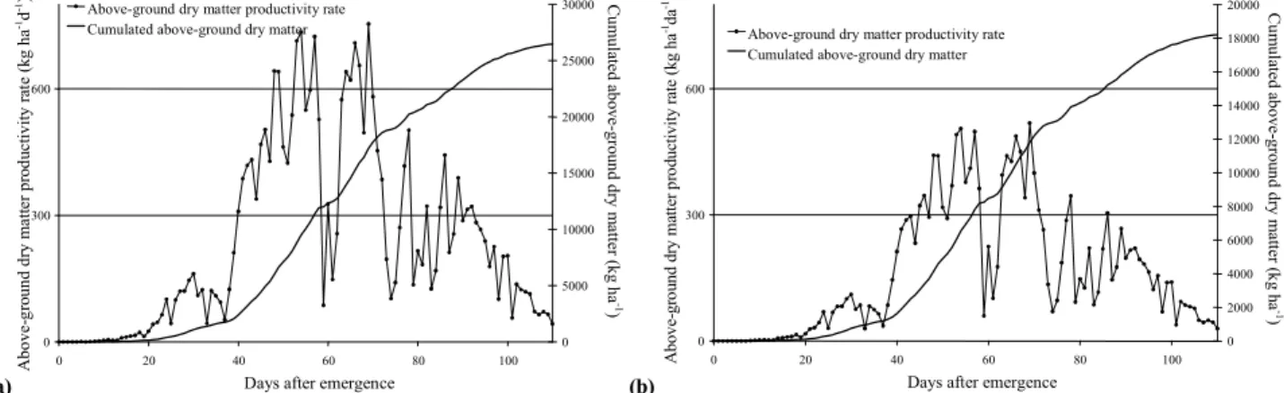
High values of above ground dry matter productivity rates during some days of flowering can be supported by coincidences of high values of air temperature with greater leaf area index values during the flowering period. Even so, full cover canopy is subjected to abrupt reductions in terms of productivity rates if climate conditions are not favorable for plant development, as shown near 60 days after emer gence (figs. 4a and 4b). Extremely high values of produc tivity rates are not frequent in agricultural practice because irrigation and other non controlled variables are rarely con trollable for the purpose of achieving such desirable com binations. The experimental data were simulated through APSIM (APSRU, 2007), and there were no water or nitro gen stresses throughout the entire maize cycle, according to APSIM released indexes. Thus, we point out that the productivity rates verified in the field experiment are relat ed to potential conditions of plant growth and development, although different environmental situations could lead to different potential productivities for maize, in agreement with Dobermann et al. (2003).
On the other hand, if maize was grown under a 25% wa ter deficit uniformly distributed throughout a cycle (i.e., Sw = 0.75 and thus Fd = 0.69), there would be a 30.26% yield reduction, as grain productivity would be 7,303 kg ha1 (fig. 4b) instead of 10,620 kg ha1. This “what if” question is not realistic for non irrigated cases because soil water continu ously fluctuates throughout the entire growing season. However, as long as there is a necessity for controlling soil water contents due to reducing water allocations in irrigated agriculture, the assumption of a 25% water deficit could
(a) (b)
Figure 4. Variation of simulated above(ground dry matter productivity rate and cumulated productivity as functions of days after emergence: (a) Sw = 1 and (b) Sw = 0.75.
0 300 600
0 20 40 60 80 100
Days after emergence
A b o v e g ro u n d d ry m at te r p ro d u ct iv it y r at e (k g h a 1d 1) 0 5000 10000 15000 20000 25000 30000 Cu
m u la te d a b o v e g ro u n d d ry m at te r ( k g h a 1 )
Above ground dry matter productivity rate Cumulated above ground dry matter
0 300 600
0 20 40 60 80 100
Days after emergence
0 2000 4000 6000 8000 10000 12000 14000 16000 18000 20000C u m u la te d a b o v e g ro u n d d ry m at te r ( k g h a 1 )
Above ground dry matter productivity rate Cumulated above ground dry matter
provide different results in terms of an economic viability extrapolation. For example, what is the magnitude of yield and therefore the income that could be achieved by reduc ing the water levels by 25% as a result of a reduced water allocation imposed by a government? Would it be viable to irrigate the crop under this situation? Technically, soil water devices allow for the checking and controlling of soil water levels with good accuracy, so that setting the level of soil water is somewhat reasonably manageable today (i.e., irri gation precision).
One source of error in figure 4b could be the assumption of a constant k (eq. 17). As k varies with LAI, especially during the early stages, Meinke (1996) showed for wheat that in situations where a high leaf area can be achieved, the slight underestimation of early dry matter production by conventional simulations that use a constant k has no sig nificant consequences for dry matter production at anthesis, unless the constant k is substantially underestimated. How ever, in situations where maximum LAI values are low, as is frequently the case in dryland production areas, cumulat ed dry matter (i.e., until anthesis) can be significantly un derestimated. The value of light coefficient extinction should be considered in every simulation model (Monteith, 1965; Jones and Kiniry, 1986; Meinke et al., 1997). For ex ample, the software APSIM 5.2 (APSRU, 2007) assumes a constant k = 0.45 for maize. Another difference is that APSIM (APSRU, 2007) also considers non continuous functions for describing TT (i.e., TT described linearly and for more than one condition), different from the function of equation 18, which is continuous.
The curve in figure 4a was simulated for non limiting conditions of water and nitrogen. It can be compared to an explanatory curve derived from experimental data by Detomini (2008). The explanatory (statistical) model was fitted to a sigmoidal curve with three parameters (p < 0.05, F test = 5083.07, and r2 = 0.9866). By comparing the de terministic model curve (for non limiting conditions) and explanatory model curve, it can be seen in figure 5 that the former (shown in fig. 4a) tends to underestimate the cumu lated above ground dry matter during the initial stages of the maize cycle and overestimate it after these stages.
According to the comparison (fig. 5) between the deter ministic model curve and the explanatory model curve fit ted from field experimental data, it is presumed that the model satisfactorily simulates maize grain productivity (Wg, kg ha1), although the above ground dry matter productivity rates (Wpa, kg ha1 d1) and the cumulated above ground dry matter (W, kg ha1) are either underesti mated or overestimated in some specific stages throughout the time course of the maize cycle. The time courses (daily basis) shown in figures 4a and 4b express the natural be havior of maize growth as a whole and confer a correct bi ophysical meaning to the model, in agreement with results obtained by Verdoodt et al. (2004). The values implied on the curves are also realistic. Therefore, the evaluation of the model through deterministic simulation and comparison of the models with field experiment observations enable the implementation of stochastic procedures on the determinis tic model.
It is convenient to mention that the model assumes that there is no nutrient stress during the crop cycle. Soil fertili ty is considered to be sufficiently upgraded to such a level that it is not necessary to be concerned about it when mi cronutrients are correctly supplied. This is very realistic be cause farmers engaged in professional agriculture generally search for necessary corrections to all soil nutrient shortag es prior to sowing the crop. In doing so, they are only con cerned about maintaining adequate nitrogen levels to the set plant population management variable. On the other hand, the model simulates the nitrogen requirement for all simu lated yields and outputs only the most likely maximum and minimum requirements. This nitrogen model relies on many input parameters and was not considered in this arti cle. Nitrogen requirement is actually one of the outputs of the model.
STOCHASTIC SIMULATIO S
Several values of daily average solar radiation and daily average air temperature are possible, but there is a corre sponding probability for each one of the daily values ac cording to the distribution to which they are likely to be fit. As a consequence, maize dry matter productivity rates and grain productivity can also vary. A stochastic procedure would approach these variations toward the identification of not only a single value but also the various classes of grain productivities associated with their corresponding probabilities. The generation of thousands of pseudo random numbers is the beginning step and, particularly for the case of the model presented here, works to generate in put values of solar radiation and air temperature according to either a bivariate normal distribution or a triangular dis tribution (if no climate series data are available) and also to generate the harvest index according to a triangular distri bution. Finally, thousands of above ground dry matter productivity rates and dry matter accumulations would have to be generated, regardless of single curves, as pre sented in figures 4a and 4b. For convenience, histograms of maize grain productivity are presented instead.
Ideally, the necessity of testing the multivariate normali ty hypothesis becomes explicit when a researcher intends to
Figure 5. Comparison between deterministic model curve and explana( tory model curve (statistically fitted from field experimental data).
0 5000 10000 15000 20000 25000
0 5000 10000 15000 20000 25000
Wpa (kg ha1): Fitted (explanatory) model 1:1
W
p
a
(
k
g
h
a
1):
D
et
er
m
in
is
ti
c
m
o
d
evaluate whether the presupposed conditions were met in terms of the inference validation that will be done. The ex istence of a “most suitable” multinormality test has been always undermined (Cantelmo and Ferreira, 2007), such as the test based on asymmetry and kurtosis deviation (Mardia, 1975) or the test based on Shapiro Wilk generali zation (Royston, 1983). Nevertheless, Mecklin and Mundfrom (2004) reinforced that a single method is not sufficient to approach the multinormality issue and that it is appropriate and even useful to run multiple tests together from an applied statistical perspective. For these reasons, the model proposed herein is pragmatically not subjected to a previous test before releasing a value of radiation or tem perature to start the stochastic simulations.
The existence of a multivariate normal distribution im plies the existence of evenly distributed marginal distribu tions, although the combined distribution of two variables that follow two separate, normal, univariate distributions does not necessarily follow one normal, multivariate distri bution. According to Hair et al. (2005), in the case in which a univariate normality presupposition is not violated, this distribution will not necessarily result in an acceptance of multivariate normality, although it will help to obtain mul tivariate normality. Therefore, if one variable follows a multivariate normal distribution, it is also univariate such that the simulation of climate data through a bivariate nor mal distribution will favor the non rejection of multivariate normality.
The most likely grain productivity for case 1 was 10,604 kg ha1 (11.53% probability) according to figure 6a, which is very similar to the productivity simulated using deter ministic conditions for Piracicaba. Probabilities around 0.02% were verified for both extreme (maximum and min imum) grain productivities (magnitudes of 12,673 and 8,634 kg ha1, respectively). One peculiarity of a normal distribution is that the grain productivity average is also the most likely value to occur, as the average is equal to the mode. If climate data were not available, one could use a triangular distribution. There is an unknown correlation in this situation, in principle, given that there is no dataset. Because of this, it makes no sense to run an adherence test such as the Kolmogorov Smirnov (non parametric) or chi squared (parametric) test, in spite of the reciprocal situation being true, i.e., from a dataset, it would be possible to fit the data to a triangular distribution and run the tests.
When simulating maize grain productivity from a trian gular distribution, the highest probability (11.5%) corre sponds to the achievement of around 11,000 kg ha1. By se lecting case 2, the grain mode becomes 400 kg ha1 greater than that of case 1, and the “shape” of the histogram in fig ure 6b is not as symmetric as the other mentioned simula tion situations. The small increase in productivity can be justified because, for most of the days of a crop cycle, both solar radiation and air temperature triangular distributions eventually allow the computation of productivity rates greater than those computed when a bivariate normal dis tribution is used. This computation is acceptable because there is an implied error in using a triangular distribution, as the mode, maximum, and minimum values are kept con stant throughout the maize cycle, which is, indeed, not true.
By keeping the water supply conditions constant but re ducing the sowing density to 5 plants m1 (i.e., reducing the plant population by ~11,111 plants ha1 as a consequence), the resulting histogram shows a productivity break around 2191 kg ha1, which is roughly 20% smaller than the poten tial productivity achieved in case 1, as can be seen in figure 6c. Provided that the plant population is kept as previously mentioned and the water level supply is reduced to 75% (Sw = 0.75 and Fd = 0.69), the model simulates a mode of 7,576 kg ha1 (11.97% probability) for grain depleted productivity (fig. 6d). As a conclusion, the model reveals that the best decision in a case of water scarcity would be to reduce the population instead of irrigating with a 75% wa ter deficit, at least for the reductions in both population and water supply tested here. It is certainly in this way that models are useful, i.e., they allow for the determination of how much a change in a variable affects the output to aid in assertive decision making.
All the histograms shown in figure 6 are based on simu lated production data. Measured crop yield or production data do not behave typically like a Gaussian distribution (unlike the histograms in fig. 6). Nevertheless, measured or production data are often not sufficient in number of obser vations to build a large sample (i.e., a sample with 10,000 observations). As mentioned in the Materials and Methods section, the central limit theorem states that if a sample is too large, then variance is minimized by trending to zero, leading a variable to approximately follow a normal distri bution (i.e., strongly bell shaped) even for non normal populations.
Although harvest index values have been simulated by a triangular distribution, it might be seen that all histograms of yield frequency prevail with a normal distribution shape. This is in part expected because driving variables of solar radiation and air temperature are both simulated to follow normal distributions. On the other hand, the smaller the amplitude of HI (maximum simulated value of HI minus minimum simulated value of HI), the smaller the resulting range of Wg values. Extremely high values (i.e., a right “tail” of the histogram) of maize grain productivity are likely to occur due to, for example, the least likely and least frequent combinations among optimal air temperature, more intense radiant regimes, and high harvest index val ues. On the contrary, a left tail is obtained. The grain productivity mode represents the central portion of the his togram and is derived from the most likely values of solar radiation and air temperature frequently combined through out the maize cycle. Additionally, there is a possibility of simulating an extremely high value of solar radiation for a given day and simulating an extreme low value for the day after, which can be physically meaningless. This misrepre sentation would be repaired by equation 25, considering that 10,000 pseudo number values are enough.
example, the weather station is some dista the specific crop location or because differe used to log data and compute daily averag purposes of stochastic approaches is thus to count for errors such as these.
GE ERAL CO SIDERATIO S
One particularity of the herein presented a stochastic procedure is that it exhibits so with Dutch generic growth models, which approached by Ittersum et al. (2003), as car similation was taken into account and th phenological events was not considered. T
(a)
(c)
Figure 6. Maize grain productivity histograms con distribution for solar radiation and air temperature air temperature under no(water(deficit conditions deficit conditions (case 3), and (d) consequence of u (case 4).
e distance away from different methods are averages. One of the hus to statistically ac
ented model that uses bits some similarities which were properly s carbon dioxide as nd the prediction of red. The model also
brings some particularities with the fa els such as CERES Maize and APSIM tion processes by adopting the radiat compute above ground dry matter Moreover, the model relies on air tem variable to predict leaf area. The fam assumes only a few parameters, most or biological meaning, and it is not s types to capture photoperiod sensitivi tial in terms of kernel number and ear pirically by the specific models. Inte presented in this work considers both and mechanistic features.
(b)
(d)
s considering that plant populations are sufficiently supplied with nitro rature under no(water(deficit conditions (case 1), (b) triangular distributi tions (case 2), (c) reduction of the plant population by taking Dsow = 5 p
ce of using a water supply that is 75% of the optimal condition (Sw = 0.
the family of specific mod APSIM, as it omits respira radiation use efficiency to matter productivity rates. air temperature as the main e family of generic models most of them with physical not specific for any geno nsitivity and genetic poten nd ear rows, as is done em ls. Interestingly, the model
s both empirical specificity
nitrogen: (a) bivariate normal ribution for solar radiation and = 5 plants m(1 under no(water(