Salt marsh response to changing hydrodynamics: the case of Ancão Inlet migration (Ria Formosa coastal lagoon)

(1)

Pedro Miguel de Sousa Vinagre Amado

SALT MARSH RESPONSE TO CHANGING

HYDRODYNAMICS: the case of Ancão Inlet migration

(Ria Formosa coastal lagoon)

Universidade do Algarve

Faculdade de Ciências e Tecnologia

2019

(2)

(3)

(4)

(5)

ii

Pedro Miguel de Sousa Vinagre Amado

SALT MARSH RESPONSE TO CHANGING

HYDRODYNAMICS: the case of Ancão Inlet migration

(Ria Formosa coastal lagoon)

Master in marine and Coastal Sciences

Work performed under the supervision of: A. Rita Carrasco (Postdoc Researcher - CIMA, Universidade do Algarve) Katerina Kompiadou (Postdoc Researcher - CIMA, Universidade do Algarve)

Universidade do Algarve

Faculdade de Ciências e Tecnologia

2019

(6)

(7)

iv

SALT MARSH RESPONSE TO CHANGING

HYDRODYNAMICS: the case of Ancão Inlet migration

(Ria Formosa coastal lagoon)

Declaration of authorship of work

Declaro ser o autor deste trabalho, que é original e inédito. Autores e trabalhos

consultados estão devidamente citados no texto e constam da listagem de

referências incluída.

I declare to be the author of this work, which is original and unpublished. Authors

and works consulted are duly cited in the text and are included in the list of

references.

Faro, 30 de Setembro de 2019

________________________

Miguel Amado

(8)

v

A Universidade do Algarve reserva para si o direito, em conformidade com o disposto no Código do Direito de Autor e dos Direitos Conexos, de arquivar, reproduzir e publicar a obra, independentemente do meio utilizado, bem como de a divulgar através de repositórios

científicos e de admitir a sua cópia e distribuição para fins meramente educacionais ou de investigação e não comerciais, conquanto seja dado o devido crédito ao autor e editor respetivos.

The University of Algarve reserves the right, in accordance with the provisions of the Code of the Copyright Law and related rights, to file, reproduce and publish the work, regardless of the used mean, as well as to disseminate it through scientific repositories and to allow its copy and distribution for purely educational or research purposes and non-commercial purposes, although be given due credit to the respective author and publisher.

(9)

vi

ACKNOWLEDGMENT

First, I would like to thank my supervisors Postdoc Researcher A. Rita Carrasco and Katerina Kompiadou for giving me the opportunity to integrate this project. Thanks, for all the guidance, help and support along all this project. My sincerely gratitude.

To Prof. Dr. Óscar Ferreira for the help and counselling. As well to Prof. Dr Alexandra Cravo for all the counselling and encouragement. As well as all my professor from the master’s program. Thank you.

Would also like to acknowledge the providing of the aerial photographs obtained from the framework of the EVREST project (PTDC/MAR-EST/1031/2014), funded by FCT (Fundação para a Ciência e a Tecnologia).

To my father and brothers, thank you for following me and supporting me in one more chapter. To my grandmother, thanks for all the encouragement and support along this path.

To my godmother for all the help and support. To João (Açoriano!) for all the support and encouragement throughout all our academic journey and for its friendship. As well, to Cátia and Luana for the help and motivation. My sincerely thanks.

A huge thanks also to all my friends from the master program for all the support and the good memories from all the moments we have shared.

(10)

(11)

viii

ABSTRACT

Concerning the economic and ecological importance of salt marshes, it is of extreme importance to improve our knowledge on the physical processes involved with marsh evolution, as well as the limits and degree of interaction with the surrounding sedimentary sources. The studied salt marsh area is located fronting Ancão Inlet, in the western sector of the Ria Formosa barrier system. A 67-year time series of aerial photographs and ortho-photographs, between 1947 and 2014, was used to infer salt marsh sedimentary evolution (progression or recession) in relation to natural inlet migration and to its relocation in 1997. The following morphologies were mapped: salt marsh, tidal flat, sand banks, and inlet flood delta. The results focus on the analysis of horizontal displacement of these morphologies over time.

It was noted that in general, the Salt Marsh presents a growth of its area along time. The different stages of the Ancão inlet migration and the consequent distance to the inlet throat is a limiting factor for salt marsh growth. The sand banks and flood deltas are the main sediment feeders of the Tidal Flat growth. The contribution of the Ancão inlet to the Tidal Flat growth was more significant when the inlet starts reaching its closure phase. The growth of Tidal Flat is an opportunity for salt marsh development.

(12)

(13)

x

RESUMO

Tendo em conta a economia e ecologia dos sapais de maré, é de extrema importância melhorar os conhecimentos sobre os processos físicos envolvidos na sua evolução, bem como o conhecimento acerca dos seus limites físicos e interações existentes com as fontes sedimentares presentes no sistema. A área de estudo deste trabalho localiza se em frente a uma barra de maré, Barra do Ancão, localizada no sector oeste do sistema de ilhas barreira Ria Formosa, Portugal. Foi utilizada uma serie temporal de 67 anos de fotografias aéreas e ortofotomapas, entre 1947 e 2014, para inferir a evolução sedimentar do sapal (progressão ou regressão) em relação à migração natural da barra do Ancão e à sua relocação em 1997. Os seguintes ambientes foram mapeados: sapal de maré, planície de maré, bancos arenosos nos canais e delta de enchente da barra. A análise de resultados incluiu a análise da variabilidade horizontal destes ambientes ao longo do tempo.

No geral observou-se um crescimento na área do sapal ao longo do tempo, influenciado pela migração da barra. Os diferentes estágios de migração da barra, e consequente proximidade à barra, são fatores limitantes para o crescimento do sapal em estudo. Verificou se que os bancos arenosos no canal e o delta de enchente da barra são as principais sumidores sedimentares para o crescimento da planície de maré. A contribuição da barra para o crescimento da planície de maré é mais significativa quando a barra começa a aproximar-se da sua fase de encerramento. Este aumento na planície de mare, por sua vez, leva ao aumento da área de sapal.

(14)

(15)

xii

LIST OF FIGURES

Figure 1.1 - Ria Formosa barrier island system (top figure) and zoomed view of the study area (bottom figure), noted with a dashed line, and surrounding the areas of Ancão Inlet and adjacent salt marsh area. ... 7 Figure 1.2 - Transect of marsh and tidal flat vegetation types identified on Barreta Island: ... 9 Figure 2.1 - Example of control point selected on the georeferencing process of an aerial photograph (A.), and transformation table of the selected control points with the associated residual error (B.). ... 12 Figure 2.2 - Example concerning the flight of 1996 where it is visible the mosaicking process: Map with different Raster files Overlapping but already with georeferenced and rectified (A); Map with clipped Raster files before changing overlap settings (B); and Map with mosaic after changing overlap settings where it is visible a smoother passage between photos (C). ... 13 Figure 2.3 - Representation of the different morphology present in the study area: Salt Marsh, Marsh Detached Beach (MDB), Fish Farming, Tidal Flat, Sand Banks (SB), Flood Delta, and Barrier. ... 14 Figure 2.4- Examples of flights with partial aerial coverage of the study area. (A) Flight of 2001 representative of flights that only have coverage on the barrier islands and partial part of the Salt Marsh under study, also the case of 1999 flight; (B) Flight of 1996, red circles indicate the area with lack of coverage. ... 15 Figure 2.5 - Representation of the different sections for the Salt Marsh and Barrier morphologies, image from the flight of 2014. ... 22 Figure 2.6 - Flight of 2014 with the representation of the baseline and transects created to apply on the shorelines to calculate the rate-of-change. ... 23 Figure 2.7 - Flight of 2014 with the representation of baselines and transects corresponding to the following morphologies: Salt Marsh West section (A.), Salt Marsh East section (B.), Tidal Flat (C.). ... 24 Figure 2.8 - Flight of 2014 with the representation of the baseline and transects used to calculate change rates of the Salt Marsh (A.) and Tidal Flat (B.) boundaries fronting the Ancão Inlet; Position of the transects and representation of the Ancão inlet position in yellow (C.). ... 25 Figure 2.9 - Graphical representation of the tidal prism data obtained during the campaigns presented in Popesso et al., (2016). The dashed line represents the 4 macro-intervals defined. ... 25

(18)

xv Figure 3.1 - Representation of the root mean square error (RMSE) data and standard deviation (STDEV) for each year of flight. ... 27 Figure 3.2 – Representation of the NDVI results for the year 2008 and Salt Marsh boundary mapped in that year. ... 28 Figure 3.3 - Evolution of the East and West Sat Marsh sections areas between 1947 and 2014. ... 29 Figure 3.4 - Evolution of the Tidal Flat area, between 1947 and 2014. ... 30 Figure 3.5 - Evolution of the Marsh Detached Beach (MDB) area, between 1947 and 2014. 30 Figure 3.6 - Evolution of the Flood Delta area between 1947 and 2014. ... 31 Figure 3.7 - Evolution of the Sand Banks area between 1947 and 2014. ... 31 Figure 3.8 - Evolution of the Ancão and Barreta barrier sections areas between 1947 and 2014. ... 32 Figure 3.9 - Statistic results (WLR) representation calculated through the DSAS tool, representing the variation rates (in m/y) of the Salt Marsh boundary, mapped in the aerial images, between 1947 and 2014. The colors from red to yellow represent erosion whereas from green to blue represent accretion. ... 33 Figure 3.10 - Statistic results (WLR) representation calculated through the DSAS tool, representing the change rates (in m/y) of the Tidal Flat boundary, mapped in the aerial images, ... 34 Figure 3.11 - Variation of the lower limit of Tidal Flat and Salt Marsh, and position of the Ancão inlet and sediment deposits (area with the presence of Sand Banks and/or Flood Deltas) for each year. ... 36 Figure 3.12 - Plots of the Salt Marsh East section (A.) and Tidal Flat (B.) southwest boundary variation, with the Inlet position. ... 37 Figure 3.13 – Salt Marsh (A.) and Tidal Flat (B.) southwest boundary average variation and evolution of the Ancão Inlet tidal prism, related to the macro-intervals (a. unstable; b. equilibrium 1; c. equilibrium 2; d. critical) based on the results of Popesso et al., (2016). . 38 Figure 3.14 - A. - Area lost or gained for each of the morphologies analyzed between 1947 and 2014; B. - Percentage of preserved and gain area for each morphology, between 1947 and 2014. Flood Delta (FD), Salt Marsh, Ancão Barrier, Barreta Barrier, Sand Banks (SB), Marsh Detached Beach (MDB), Tidal Flat (TF), Secondary Channels and Others (SCO). ... 41 Figure 4.1 – Conceptual scheme representing significant morphology land-cover changes, between along all the study period (1947-2014). ... 46

(19)

xvi Figure I.1 – Tables represent the area percentage value of a morphology a in year i that transformed to a morphology b in year j. Values filled in grey represent the preserved area of each morphology, dark green represent the transitions above 50%. ... 53 Figure I.2 – Results from the probability of a land-cover change being highly significant (dark green) for each time-step. ... 54 Figure I.3 – Schematic representation of the highly significant (probability>0.05) land-cover changes for all the 10 time steps. ... 56 Figure I.4 – Representation of the different morphology present in each year of study: Salt Marsh, Marsh Detached Beach (MDB), Fish Farming, Secondary Channels and Others (SCO), Tidal Flat, Sand Banks (SB), Flood Delta, Barrier. ... 58

(20)

xvii

LIST OF TABLES

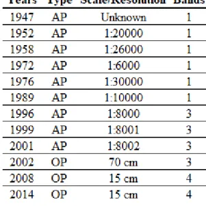
Table 2.1 - Raster data used and respective information, year of the flight, data type (i.e., aerial photo or ortho-photo, denoted AP and OP, respectively), resolution and number of bands available, are also noted. ... 10 Table 2.2 - Characterization of the diverse morphologies present in the study area. Description of the spatial limits and presence of vegetation, identification process of the morphology in the aerial images, and examples of the respective morphologies in color and in black and white aerial images. ... 16 Table 3.1 - Average of root mean square errors (RMSE) related to the georeferencing process and corresponding standard deviation (STDEV), taking into account all georeferenced aerial photos for each flight. ... 27 Table 3.2 - Mapped morphologies in each flight year. Present (x), Absent (-)... 28 Table 3.3 - The matrix describes the strength of the correlation between morphologies areas, for Flood Delta (FD), Fishing Farm (FF), Salt Marsh, Ancão Barrier, Barreta Barrier, Sand Banks (SB), Marsh Detached Beach (MDB), Tidal Flat (TF), and Secondary Channels and Others (SCO). Highlighted values denote significant correlations (green are positive and red are negative). ... 39 Table 3.4 - Representation of the percentage value of a morphology a in 1947 that transformed to a morphology b in 2014. Values filled in grey represent the preserved area of each morphology, and dark green the transitions above 50%. Flood Delta (FD), Fishing Farm (FF), Salt Marsh, Ancão Barrier (B.), Barreta Barrier (B.), Sand Banks (SB), Marsh Detached Beach (MDB), Tidal Flat (TF), Secondary Channels and Others (SCO). ... 40

(21)

(22)

xix

LIST OF ABBREVIATIONS

AP Aerial photographs

DSAS Digital Shoreline Analyse System GIS Geographic Information Systems HWL High Water Level

MDB Marsh Detached Beach

NDVI Normalised Difference Vegetation Index OP Ortho-photographs

RMS Root mean square RMSE Root mean square errors SB Sand Banks

SCO Secondary Channels and Others SLR Sea level rise

STDEV Standard deviation

(23)

(24)

1

SUMÁRIO

As áreas de sapal persistem durante milhões de anos, apesar de serem naturalmente dinâmicos, expandindo e contraindo a sua dimensão em resposta a mudanças no fluxo dos rios e na dinâmica das marés. A sua variabilidade no tempo e espaço resulta da influência de fatores abióticos, bióticos ou antropogénica. As regiões de sapal são dos ecossistemas mais produtivos da Terra. Tendo em conta a sua importância económica e ecológica, é de extrema importância melhorar os conhecimentos sobre os processos físicos envolvidos na evolução dos sapais, bem como os limites e interações existentes com as fontes sedimentares. Este estudo tem como propósito analisar a influencia da migração de uma barra de maré sobre uma determinada zona de sapal, para que no futuro possam ser tomadas decisões mais conscientes na gestão deste tipo de sistemas de maneira a deixar o menor impacto possível.

Foi utilizada uma serie temporal de 67 anos de fotografias aéreas e ortofotomapas, entre 1947 e 2014, para inferir a evolução sedimentar do sapal (progressão ou regressão) em relação à migração natural da barra do Ancão e à sua relocação em 1997. As fotografias áreas foram georreferenciadas a partir de ortofotomapas de maneira a poderem ser trabalhadas em SIG. O processo de georreferenciação foi feito dos anos mais recentes para os mais antigos de maneira a usar os ortofotomapas como base para a georreferenciação as fotografias aéreas. Sendo sempre usado como base o ano anterior mais próximo possível. Neste processo o objetivo é ter a melhor cobertura possível de pontos de controlo para ter o mínimo de distorção possível. Foram mapeados 8 ambientes sedimentares (morfologias) a partir de 11 voos disponíveis para o período em análise: sapal de maré, planície de maré, bancos arenosos nos canais, delta de enchente da barra, praias isoladas de sapal, piscicultura, parte das ilhas barreira e canais secundários e outros, que em conjunto representam a totalidade da área de estudo. O mapeamento destas morfologias tem como objetivo inferir a sua variação horizontal (m/ano), as variações sedimentares entre elas, e principalmente, a sua variação tendo em conta a posição da barra do Ancão. Relativamente ao processo de mapeamento das diferentes morfologias, foram definidas as características geomorfológicas dos seus limites, que foram tidas em conta para todos os anos. No caso específico do sapal mapeado em 2008 foi utilizada a informação infravermelha presente no voo para confirmar este mapeamento. Este processo foi realizado utilizando um índice de vegetação (NDVI) que nos dá um mapa da vegetação presente na área. No que diz respeito aos erros associados a georreferenciação das fotografias aéreas verificou-se que este é superior nas fotografias mais antigas, em resultado da dificuldade de

(25)

2

georreferenciação das mesmas devido à sua fraca qualidade, mas também a acumulação de algum erro de um ano para o outro.

A abordagem definida em Gonzalez et al. (2005), foi utilizada para validar as mudanças entre morfologias, entre dois voos consecutivos. As variabilidades morfológicas a longo termo foram também analisadas conjuntamente com macro-interválos de variabilidade no prisma de maré da Barra do Ancão, definidos por Popesso et al. (2016). Pretendeu-se associar os períodos de estabilidade/instabilidade hidrodinâmica da Barra do Ancão com o comportamento do sapal e planície de maré, nos mesmos períodos de análise.

Em geral, apenas o sapal e planície de maré apresentaram um aumento da sua área ao longo do tempo. Relativamente ao sapal de maré, a secção oeste apresentou um crescimento mais estável que a secção este. No que diz respeito à variação do limite destas morfologias, ambas apresentaram sinais de erosão ao longo do canal a nordeste, canal do Ramalhete, e acreção no limite sudoeste, nomeadamente na região afetada pela migração da Barra do Ancão.

Tendo em conta os resultados obtidos concluímos que a planície de maré é a morfologia mais importante para o aumento de área do sapal, correspondendo 4 % da área final do sapal a antiga planície de maré. As duas morfologias apresentam uma forte correlação positiva entre si, o que leva a concluir que o sapal depende indiretamente dos mesmos fatores que a planície de maré para aumentar a sua área. Estes fatores são maioritariamente depósitos sedimentares (delta de enchente e bancos arenosos) que a longo prazo levaram ao aumento da planície de maré. Que por sua vez dará oportunidade para o desenvolvimento do sapal.

Observou-se ainda que a curto prazo a migração da Barra do Ancão apresenta impactos negativos na planície de maré durante a primeira metade do seu ciclo de migração, devido maioritariamente a aportes sedimentares (delta de enchente e bancos arenosos). A formação destas morfologias leva a diminuição da planície de maré, devido tanto a sua erosão como por estas a soterrar. Isto é seguido por um período positivo com o afastamento da barra da planície de maré, dando oportunidade para esta se desenvolver ou recuperar a sua área anteriormente soterrada. Como resultado o sapal apresenta um aumento na primeira metade do ciclo de migração da barra, já depois da planície de maré ter desenvolvido, e começa a diminuir depois de a planície de maré ser afetada pela passagem da barra. Analisando estes resultados, conclui-se que a região com as condições ideais para o deconclui-senvolvimento conclui-sedimentar destas morfologias é a região imediatamente antes da barra iniciar a sua fase de encerramento. Pois esta região possui tanto a presença de sedimentos necessários para o desenvolvimento destas morfologias como as condições hidrológicas adequadas.

(26)

3 Relativamente aos valores negativos apresentados na variação dos limites de sapal e planície de maré, estes poderão ser causados por fatores naturais (correntes de maré) ou antropogénicos (ex. dragagens). Apesar da forte presença de erosão ao longo do limite destas morfologias, as suas áreas estão, na generalidade, a aumentar. O que implica que as regiões de acreção, apesar de menores em extensão, acabam por compensar estas perdas. Os resultados destas variações vêm ainda suportar que a região imediatamente antes da barra iniciar a sua fase de encerramento é ideal para o desenvolvimento de sapal, sendo esta a regiões do seu limite que apresenta maiores valores de progressão.

Em soma podemos concluir que a Barra do Ancão, a longo prazo, contribui de forma positiva para o desenvolvimento do sapal de maré. Espera-se assim com este estudo ajudar na tomada de decisões relativas a gestão desta região, assim como em outras semelhantes.

(27)

4

Chapter 1 -

INTRODUCTION

1.1. Background and Motivation

Tidal marshes are among the most productive ecosystems on Earth and provide key services including shoreline protection, water quality improvement, provision of fish habitat (Gedan et al., 2009), and carbon sequestration (McLeod et al., 2011). Marshes persist for thousands of years despite being naturally dynamic, expanding and contracting in extent and in response to changes in river flow and tidal dynamics (Redfield, 1972). Their variability across time and space results from the influence of abiotic (e.g., soil capping, type of groundcover, salinity, flood depth) and biotic (e.g., canopy cover, plant age, plant type, type of animal present) factors (Bhattacharjee et al., 2009; Day et al., 1997; Morris et al., 2002); in some cases, these alterations are induced by human activities (Day et al., 2008). A major emerging threat to marsh stability and function is the projected acceleration in the rate of sea-level rise (SLR). Some impacts of the SLR are the landward migration of barrier islands and the drowning of high-tide marshes (FitzGerald et al., 2008).

Regarding the economic and ecological importance of salt marshes, it is of extreme importance to improve our knowledge on the physical processes involved with marsh evolution, as well as the limits and degree of interaction with the surrounding sedimentary sources. This thesis intends to show the influence of the migration patterns of a tidal inlet to the sediment variability of the neighboring marsh. The work analyzes the impacts of the natural inlet migration and of the human inlet relocation, in relation to salt marsh sedimentary evolution (progression or recession). Leading to an increase of knowledge regarding salt marsh response to changing in hydrodynamic conditions due to inlet’s migration.

1.2. Goals

Two specific goals are addressed in this thesis:

• Determine the influence of Ancão Inlet natural migrating stages and human relocation to the surrounding salt marsh development, over the last 67 years.

• Determine how the diverse sand contributors (e.g., tidal flat and flood deltas) present in the lagoon system interact and influence the salt marsh development.

(28)

5

1.3. State of the Art

Recent and fundamental bibliographic information and definitions regarding the main environments, functions, and interactions present in coastal systems like the Ria Formosa are discussed in the present section, along with a short analysis of the recent evolution of the Ancão Inlet and of the neighboring marsh areas.

1.3.1. Coastal lagoons and tidal inlets

A coastal lagoon is defined as a partially isolated water body, separated from ocean by a barrier and linked to it through one or more inlets (Kjerfve, 1994). These inland water bodies have depths that rarely exceed a couple of meters and are usually parallel to the coast (Barnes, 1980). Their origin is a result of the sea level rising process during the Holocene or Pleistocene and the subsequent building of coastal barriers due to marine processes (Barnes, 1980). Using the definition of Escoffier (1977), an inlet is a short, narrow channel that connects a bay, lagoon or an estuary to a larger body of water. This connection plays an important part in several processes, like navigation, exchanges of water between two different systems, controlling temperature, salinity, dilution of different compounds present in water and fish migration. According to Bruun (1978), the origin of inlets can belong to one of the following three different groups: geological, hydrological or littoral drift origin. Tidal inlets are located within barrier island systems, present in several parts of the world, on the most diverse geological and oceanographic conditions (FitzGerald, 1988), and are formed when the flow of water is dominated by the tide as opposed to river discharge (Escoffier, 1940). The importance of the influence that tidal range has on tidal inlets and barrier morphology was first recognized by (Hayes, 1979), identifying and correlating five general categories of shorelines with the presence or absence of barrier island systems and tidal inlets (Pacheco, 2010).

A multitude of published work exists regarding the recent morphological evolution of the Ancão Inlet and surrounding barriers (Ancão Peninsula and Barreta Island), as for example Pacheco et al. (2010), Vila-Concejo et al. (2004 & 2006) and Dias et al. (2009). However, very little is known on the impacts of the inlet changes (migration, relocations and related changes to hydro- and sediment dynamics) to the evolution of the marsh present in this area. There are some works regarding the impact of the Ancão Inlet to the seagrass landscape (Cunha et al., 2005; Cunha and Santos, 2009). With this work we pretend to add more information regarding the impact of the Ancão inlet migration on the salt marsh but also in the surrounding morphologies, and how these interact with each other taking into account the Ancão inlet migration cycle. This supports the originality and the purposefulness of the proposed work.

(29)

6

1.3.2. Tidal marshes

Regarding tidal marsh evolution, many biotic and abiotic factors can influence its condition and expansion, like sediment supplies, sea levels, eutrophication, grazing, temperature, salinity, as well as various anthropogenic pressures (Bhattacharjee et al., 2009; Raposa et al., 2016). Given that tidal marshes occupy a narrow elevational range, that broadly extends from mean sea level to the upper limit of spring high tide, one critical parameter to marsh stability and function is the balance between sediment supply and sea levels (Raposa et al., 2016): wetland plants drown if inundated excessively and are replaced by upland species if inundated insufficiently. Thus, coastal wetlands persist in their current locations only if they are able to build vertically at a rate equal to or greater than the rate of SLR (Arnaud-Fassetta et al., 2006). Their ability to do so may be inhibited by human alterations, such as decreased riverine sediment supply or increased subsidence rates (Day et al., 2008; Kirwan and Megonigal, 2013; Morris et al., 2002). Another mechanism through which coastal wetlands cope with accelerating sea levels is to migrate to new, higher positions. However, in many regions, including Ria Formosa, built structures and urban development along the inland boundary of the lagoon inhibit this migration, leading to constraining of marsh endurance in conditions of increased SLR and/or accelerated sediment supply, often referred to as coastal squeeze (Pontee, 2013; Vinent et al., 2019). Vila-Concejo et al. (2003) conducted a monitoring program, including the acquisition of a series of topo-bathymetric surveys and oblique aerial photos presenting morphological and volumetric results, as well as inlet channel evolution and tidal delta formation. The study of Popesso et al. (2016), concerning the natural migration evolution after the relocation, showed that southwestern storm events can increase the sediment longshore supply and help migration, while events coming from the east and from directions more perpendicular to the shoreline can fill the flood deltas and disrupt the eastward migration. Showing also that constant longshore transport is the major driver of migration continuity, and the main storms are the drivers of rapid migration events or migration by jumps.

Ancão Inlet relocation had several advantages, such as decreasing water pollution due to better water renewal, and increasing the inlet stability (Dias et al., 2009). However, significant environmental impacts could overcome from this intervention, as suggested by a study lead by Cabaço et al. (2010), who argue that the inlet relocation, along with channel dredging, may have altered the landscape distribution of Cymodocea nodosa meadows in Ria Formosa. It is important to keep in mind that any human action, even the ones concerning soft protection techniques, must be considered as leaving a durable imprint to the environment, creating new conditions compared to the ones existing in the past (Carrasco et al., 2012).

(30)

7

1.4. Study Area

Ria Formosa coastal lagoon, located in the Algarve region (Faro), in the southern coast of Portugal, is protected by a multi-inlet barrier island system (Figure 1.1). The barrier system is presently composed of five islands (Barreta, Culatra, Armona, Tavira, Cabanas) and two peninsulas (Ancão, Cacela) separated by six tidal inlets (Ancão, Faro-Olhão, Armona, Fuseta, Tavira, Lacém), responsible for water exchange between the lagoon and adjacent sea. The lagoon has a triangular shape, about 55 km length (E-W) and 6 km width (N-S) in its widest zone. It contains around 105 km2 of wet area, including a large intertidal zone (Dias et al., 2009).

Figure 1.1 - Ria Formosa barrier island system (top figure) and zoomed view of the study area (bottom figure), noted with a dashed line, and surrounding the areas of Ancão Inlet and adjacent salt marsh area.

Wave directions are usually from W-SW, corresponding to 71 % of incidences, while 24 % represent waves coming from E-SE. Tides are semi-diurnal, with an average range of 1.3 m during neap tides and an average range of 2.8 m during spring tides that can reach 3.5 m (Costa et al., 2001), corresponding to mesotidal conditions. The wave energy regime is moderate to high and mean annual Hs (significant wave height) for offshore waves is 0.92 m (Costa et al., 2001).Due to its shape, Ria Formosa comprises two different flanks in terms of wave exposure

(31)

8

(Costa et al. 2001). The western flank, where the study area (Ancão Peninsula and Barreta Island) is located, is the more energetic one, being under the direct influence of the dominant wave conditions (Vila-Concejo et al., 2004).

The lagoon and back barrier environments of Ria Formosa are characterized by (a) large salt marsh areas with a dense distribution of shallow meanders, composed of silt and fine sand (Bettencourt, 1994), (b) large sand flats, partially flooded and reworked during spring tides (Pilkey et al., 1989; Carrasco et al., 2008), and (c) a complex network of natural and partially-dredged channels, which narrow and shoal in the upper regions of the system (Salles, 2001). Ria Formosa is a Natural Park, holds target habitats for conservation (EU Habitat Directive) and is protected by Natura 2000. It supports the reproduction and development of oceanic species and mollusks, with an important economic interest. It also constitutes a valuable regional resource for tourism, fisheries, aquaculture, and salt extraction industries, as well as a natural habitat for various species of birds (Dias et al., 2009).

Regarding marsh vegetation in Ria Formosa, it has developed over nearly flat zones of sandy and clayey sediments of marine origin; two main vegetation types are present: halophytic in the submerged and saline wetlands and psamophilic in the dunes and pine forests (Costa et al., 1996), similar to the ones represented in Figure 1.2. The long (1941-2000) and short-term (2000-2002) evolution of the marsh in the western part of the study area (near Quinta do Lago footbridge) was investigated by Arnaud-Fassetta et al. (2006), who determined vertical accretion rates of 8 to 9 mm/y for the long-term and vertical erosion rates of -9 to -3.7 mm/y for the short term evolution; this negative rates could indicate that salt marshes could become unable to compensate the effects of SLR.

The studied salt marsh area is located on the west part of Ria Formosa, north from the Ancão Peninsula and the Ancão Inlet (Figure 1.1). The evolution of the studied salt marsh area possibly presents a close relation with the Ancão Inlet migration and evolution patterns, however, to present no studies were conducted to prove and quantify, or to disprove this relation. This inlet presents a progressive easterly migration, result of the alongshore sediment transport from west to east due to the dominant sea conditions (Pilkey et al., 1989), and an ebb-dominated behavior (Salles, 2001; Vila-Concejo et al., 2004). Each migration cycle starts with the inlet opening in a western position, followed by its eastward migration, with a mean rate of ~67 m/y (Dias et al., 2009). The cycle ends with the inlet reaching its most eastern position and finally closing, which leads back to the beginning of another cycle, with the opening of a new inlet in, or near, a former western position (Dias et al., 2009; Pilkey et al., 1989).

(32)

9 The natural eastward migration pattern of Ancão Inlet caused in the past restrictions on navigation and water exchange through the inlet, that led to the decision of relocation in a western position in June 1997, to improve its hydrodynamic efficiency (Vila-Concejo et al., 2004). The post-intervention evolution of the inlet has been studied extensively.

Figure 1.2 - Transect of marsh and tidal flat vegetation types identified on Barreta Island: 1. Salsalo kali-Cakiletum maritimi 2. Euphorbio paraliae-Agropyretum junceiformis 3. Loto

cretici-Ammophiletum australis 4. Artemisio crithmifoliae-Armerietum pugentis 5. Ononidi variegatae-Linarietum pedunculatae 6. Frankenio laevis-Salsoletum vermiculatae elymietosum boreali-atlantici 7. Polygono equisetiformis-Limoniastretum monopetali 8. Cistancho phelypaeae-Suaedetum verae 9. Inulo crithmoidis-Arthrocnemetum glauci 10. Halimiono portulacoidis-Sarcocornietum alpini 11. Sarcocornio perennis-Puccinellietum convolutae 12. Spartinetum maritimae 13. Zosteretum nolti 14. Cymodoceetum nodosae.

(33)

10

Chapter 2 -

METHODS

2.1. Treatment of Aerial Photographs

2.1.1. Available Datasets

This work is based on the analysis of aerial images to determine the horizontal spatial evolution of the salt marsh and of the morphologies around it that may, or may not, influence its evolution. The analysis focused on an average long-term approach (years to decades) of the changes that occurred over 67 years of study, between 1947 and 2014. The available data are of two types, aerial photographs (AP) and ortho-photographs (OP) (Table 2.1).

The ortho-photographs are already georeferenced and ortho-rectified, that is, the image already has true geographic information and is already corrected for optical distortions, such as tilt, relief, and lens distortion. The same is not true for aerial photographs. These photographs are raster images that need to be georeferenced and rectified, in order to be used in GIS.

Table 2.1 - Raster data used and respective information, year of the flight, data type (i.e., aerial photo or ortho-photo, denoted AP and OP, respectively), resolution and number of bands available, are also noted.

(34)

11 2.1.2. Georeferencing and Rectification

As mentioned previously, aerial photographs, unlike ortho photographs, are simple raster images, with no associated geographic information and subject to inherent errors related to distortion and displacement. To add geographic information on the raster images and to correct errors, ortho-photographs are used as a base map, overlapping the raster image that is going to be corrected on top. This process is accomplished by selecting a set of ground control points, these are visual references that are identifiable in both photographs (aerial photo and ortho-photo). The idea is to use a georeferenced and rectified base map close to the year of the aerial photos that are going to be georeferenced, to have the minimum changes in landscape and to simplify the choice of suitable control points. Thus, the georeferencing process is performed “backward” in time, going from the most recent to the oldest photographs. Generally, the basis for the georeferencing of each flight is the directly posterior, available, flight. The ortho-photograph of 2002 was used as the basis for the georeferencing process, as it is the oldest available flight ortho-rectified of Ria Formosa. Thus, the orthographic of 2002 was used to georeferencing the aerial photograph of the previous year available (2001). In turn, photographs of 2001, after georeferenced and rectified, were used as a base for the flight of 1999, and so on. To rectify the raster images, it is important to take into account errors associated with: (a) distortion, that is any shift in the position of an image on a photography that alters the perspective characteristics of the image, and (b) displacement, which is any change in the position of an image in a photograph that does not alter the perspective characteristics of the photography (Kombiadou and Matias, 2017; Paine and Kiser, 2012).

According to Paine and Kiser (2012), the main causes of changes in aerial photography are: Lens distortion - diffusion from the main point that makes an image look closer or farther than it actually is at this point. By calibrating the lens, a distortion curve can be obtained that shows how the distance varies with the diffused distance from the main point. This information can be applied to fix the distortion of the lens if it is known to distance between the main point and the position of a point in the image.

Tilt displacement – tilt is caused due to the plane or other aerial platforms not being perfectly horizontal at the time of exposure. This can be corrected if the direction and value of tilt are known.

Topographic displacement – it radiates from the nadir and can be removed using stereoscopy. It can calculate this offset and apply corrections to specific points. This displacement has a positive side that allows the interpretation of pairs of stereoscopic photos in three dimensions, obtaining heights and topographic maps using aerial photography.

(35)

12

To correct these distortion problems, a second-order transformation is used in the georeferencing process. So it is necessary that the ground control points used are well distributed throughout the entire photo area, to avoid forcing distortions due to the level of the transformation used. It is important to have a good coverage at least of the barrier and salt marsh which are the areas of greatest interest, so they can not suffer any kind of distortion.

Control points must be carefully selected to avoid tilt errors. To do this, priority was given to control points near the ground (e.g. marsh morphological features, pothole vegetation) that correspond to the same point throughout the years and not to ones having seasonal variation. In the case of rapid changes in the landscape between flights, or lack of such features, the selection of such points is not possible and using tall structures as control points is inevitable. In this case, the point nearest to the ground is selected, to avoid relief displacement.

When the selection of the control points is done, a transformation table is created, with the values of the associated root mean square (RMS) error, according to the transformation applied (see example Figure 2.1). The RMS error represents the square root of the average square of the distance between the control point selected on the base map and the point selected on the rectified raster (under georeferencing), applying the regarded transformation. Essentially, it corresponds to the mean displacement of the georeferenced photo in comparison with the base map. In this case, in order to achieve the greatest possible accuracy, it is considered important that this error is as low as possible. Processing of aerial photographs was performed using a GIS software.

Figure 2.1 - Example of control point selected on the georeferencing process of an aerial photograph (A.), and transformation table of the selected control points with the associated residual error (B.).

(36)

13 2.1.3. Mosaicking and preparation of photos for interpretation

After the previous step and although all the photos have geographic information and the necessary corrections, they are still individual raster files. This means that each year of flight has several files representing the entire area of study (Figure 2.2 A), which makes it difficult to visualize and interpret photos due to overlays.

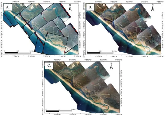
To simplify the whole interpretation process that follows it was necessary to edit the images and join them in a single file. In order to have a better view of the photos together, the frame of each photo is removed leaving only the relevant area. Then all the individual photos belonging to the same flight are included in a mosaic (Figure 2.2 B). To finish the mosaic settings are changed so that there is a smoother passage between photos (Figure 2.2 C). This process simplifies the visualization of the mosaic, where all images of a particular flight are grouped, helping in the analysis to be carried out.

Figure 2.2 - Example concerning the flight of 1996 where it is visible the mosaicking process: Map with different Raster files Overlapping but already with georeferenced and rectified (A); Map with clipped Raster files before changing overlap settings (B); and Map with mosaic after changing overlap settings where it is visible a smoother passage between photos (C).

(37)

14

2.2. Aerial Image Interpretation

2.2.1. Mapping of Different Morphologies

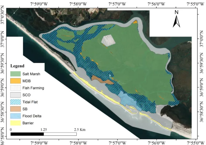
This analysis considers different types of morphologies (Figure 2.3), present in the study area. The studied morphologies, apart from the Tidal Flat that may appear with or without vegetation, can belong to two different categories, vegetated and non-vegetated. For this analysis, a vegetated morphology presents a dense and continuous vegetation throughout its entire area, and non-vegetated morphologies occurs where vegetation is not visible, or when it is very dispersed throughout the entire area. In total, seven distinct morphologies were defined: Salt Marsh, Marsh Detached Beach (MDB), Fish Farming (FF), Tidal Flat (TF), Sand Banks (SB), Flood Delta, and Barrier. For a better understanding of the different morphologies and their spatial limits, morphological details were placed on Table 2.2.

Figure 2.3 - Representation of the different morphology present in the study area: Salt Marsh, Marsh Detached Beach (MDB), Fish Farming, Tidal Flat, Sand Banks (SB), Flood Delta, Barrier, Secondary Channels and Others (SCO).

Considering that the submerged morphologies (Tidal Flat, Sand Banks (SB), Flood Delta) are highly dependent on the tide level at the time of the flight, there may be some difficulties in their cartography and interpretation. Therefore, special attention was needed when working with these morphologies. Cases, where the tidal level has obstructed, or prevented this process,

(38)

15 have been noted, and are to be considered at the time of results interpretation. Also, cases, where the quality of the image prevented a good interpretation of the different limits, were noted, as well as cases where there was some natural phenomenon that makes some impediment of interpretation, by example water surface reflectivity.

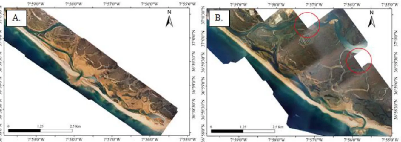
In cases where it was impossible to mark the different limits, the limit of the previous flight was used, only if they do not have a large time space with each other, are marked correctly and do not present a large horizontal spatial variation between flights. For example, the flights of 1999 and 2001 only have coverage on the barrier islands and partial coverage of the Salt Marsh under study (Figure 2.4 A). In the case of the 1996 flight, there is only missing coverage in two edges of the Salt Marsh (Figure 2.4 B). However, it have a good marking of this areas in 2002, and since this is close to the years lacking aerial coverage, its limits are used to complete the lacking information of the others. When the delimitation of a morphology was not possible, it was discarded from the analysis.

Figure 2.4- Examples of flights with partial aerial coverage of the study area. (A) Flight of 2001 representative of flights that only have coverage on the barrier islands and partial part of the Salt Marsh under study; (B) Flight of 1996, red circles indicate the area with lack of coverage.

(39)

16

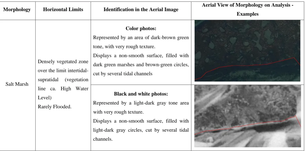
Table 2.2 - Characterization of the diverse morphologies present in the study area. Description of the spatial limits and presence of vegetation, identification process of the morphology in the aerial images, and examples of the respective morphologies in color and in black and white aerial images.

Morphology Horizontal Limits Identification in the Aerial Image Aerial View of Morphology on Analysis - Examples

Salt Marsh

Densely vegetated zone over the limit intertidal-supratidal (vegetation line ca. High Water Level)

Rarely Flooded.

Color photos:

Represented by an area of dark-brown green tone, with very rough texture.

Displays a non-smooth surface, filled with dark green marshes and brown-green circles, cut by several tidal channels

Black and white photos:

Represented by a light-dark gray tone area with very rough texture.

Displays a non-smooth surface, filled with light-dark gray circles, cut by several tidal channels.

(40)

17 Tidal Flat

Intertidal zone (below the intertidal-supratidal limit; High Water Level) that can be vegetated or not, can border Salt Marsh or MDB morphologies. Lower limit extends to the edge of the tidal channel, sand bank or flood delta.

Flooded along the tide cycle depending on the tidal level on each flight.

Color photos:

Represented by a brown-green color area when non-vegetated, and dark brown-green color area when vegetated. It displays an apparent smooth texture and is not often cut by tidal channels.

Represented by an area of light gray color when non-vegetated and by dark gray-black when vegetated. It displays an apparent smooth texture and is not often cut by tidal channels.

(41)

18

MDB

Sandy isolated areas, inside the upper Salt Marsh, above the maximum level of spring tide.

These zones do not flood.

Color photos:

Represented by an area of yellow tone, with apparent roughness and scarce vegetation, aggregated in small tufts separated from each other.

Represented by an area of light white-gray tone with apparent roughness and scarce vegetation, aggregated in small tufts separated from each other.

(42)

19 Sand Banks

Intertidal sandy areas, not vegetated, located in the tidal channels and on top of (older) Tidal Flat.

Color photos:

Represented by an area with light yellow-brown tone. Displays a smoothed surface, but with little roughness. Visually, it appears as an elongated deposition surface with different shapes of ripples.

Represented by an area with light white-gray tone. Displays a smoothed surface, but with little roughness. Visually, it shows up as an elongated deposition surface with different shapes of ripples.

(43)

20

Flood Delta

Intertidal sandy areas in the lagoon-side, not vegetated, fronting the (ebb) tidal inlet (usually north of the inlet).

Color photos:

Represented by an area with light yellow-brown tone. Displays a smooth surface with little roughness. Visually, it is shown as a fan-shaped deposition surface. It includes abandoned parts, shaped like a distorted fan and with more tidal channels and sometimes with darker color.

Represented by an area with light white-gray tone. Visually, it is shown as a fan-shaped deposition surface. It includes abandoned parts, shaped like a distorted fan and with more tidal channels and sometimes with darker coloring.

(44)

21 Barrier

Sandy barrier zone vegetated or not. Delimited by the ocean and the lagoon-side coastlines zone (debris line; ca. HWL).

Color photos:

Represented by a line (debris) with light yellow-brown tone. Displays some apparent roughness.

Represented by a line (debris) with shades between white and light gray. Displays some apparent roughness.

(45)

22

2.2.2. Spatial Variation

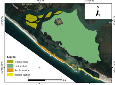
The mapping done at the previous point is used to get the total area of each individual morphology, for all years where mapping was possible to perform. The value is acquired calculating the area of the polygon representative of each morphology. In the case of Salt Marsh, the total area is divided into two sections, East and West (Figure 2.5). The West section is composed by six Salt Marsh islands located in the most western part of the study area. The total area of the Marsh morphology is the sum of both sections. This would allow a comparison between both sections, or between one of them with another morphology. The same happens for the Barrier total area, were we have Ancão barrier section and Barreta barrier section (Figure 2.5). The total barrier morphology area is the sum of both Ancão and Barreta sections. Regarding the MDB and Sand Banks morphologies, the total area of each one is the result of the sum of the areas of all mapped polygons, representative in each flight.

The total study area, sum of all mapped morphologies previously defined (Figure 2.3), was also delimited in order to obtain its total value (stable in time). The area resulting from the subtraction of all morphologies to the total study area represents Secondary Channels and Others (SCO).

The computed areas are used to test the existence of a possible correlation between the different morphologies. Moreover, these values are used to check for the horizontal spatial evolution of each morphology over the 67 years, calculated from the difference between the same morphology from two consecutive years of flight.

The polygons representative of the non-vegetated morphologies, Flood Delta and Sand Banks are used to assess changes in the rate of sedimentary availability (m2_{/y) between flights (i.e. by} adding total sand for each flight).

Figure 2.5 - Representation of the different sections for the Salt Marsh and Barrier morphologies, image from the flight of 2014.

(46)

23

2.3. Computing Boundary Change Rates

2.3.1. Variation Rates of the Salt March and Tidal Flat boundary

DSAS tool (Thieler et al., 2009) is a user-friendly interface, making it possible and easy to calculate shoreline rate-of-change statistics from multiple shoreline positions along a given period. This calculation is done using transects created by the program and defined by the user. For this study, a spacing of 50 meters has been used between transects, whose length had to be adjusted so that each existing transect cut across the boundary line of all years presents (Figure 2.6).

Figure 2.6 - Flight of 2014 with the representation of the baseline and transects created to apply on the shorelines to calculate the rate-of-change.

Transects generated by DSAS can be used to calculate the following change metrics: Distance measurements (Shoreline Evolution Changes; Shoreline Movements) and Statistics (End Point Rate; Least Squares Regression; Weighted Least Squares Regression; Supplemental statistics for Least and Weighted regression; Confidence Interval; Standard Error; R-squared). The software includes a manual with detailed instructions for defining the baseline, generate automatic or manual transects, and other data based on parameters specified by the user. Therefore, is suitable to calculate shoreline rate-of-change for any type of environment over a given period. (Thieler et al., 2009).

(47)

24

The ‘shorelines’ used to run the DSAS are the boundaries of the mapped morphologies. This approach is only applied to Salt Marsh and Tidal Flat boundaries, to obtain their rate-of-change for the entire study period. The Salt Marsh morphology was divided into two different sections, following the same logic as in the calculation of the areas (Figure 2.7).

Figure 2.7 - Flight of 2014 with the representation of baselines and transects corresponding to the following morphologies: Salt Marsh West section (A.), Salt Marsh East section (B.), Tidal Flat (C.).

2.3.2. Salt March and Tidal Flat change rates, fronting the Ancão Inlet

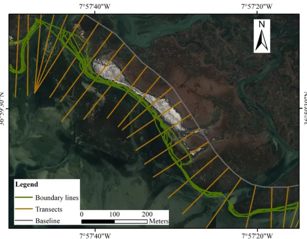
These analyses consist in using the DSAS tool to calculate change rates of Salt Marsh and Tidal Flat boundary, considering the inlet position in each year of flight. To this end, a baseline was created, as parallel as possible to the Salt Marsh and Tidal Flat boundaries fronting the Ancão Inlet. The transects are cast with a spacing of 50 meters and with a length large enough to cross the boundaries of all years (Figure 2.8 C.). On each flight, the transect closest to the center of the inlet was used to identify its position at the time of the respective flight (yellow transect in Figure 2.8 C).

(48)

25 Figure 2.8 - Flight of 2014 with the representation of the baseline and transects used to calculate change rates of the Salt Marsh (A.) and Tidal Flat (B.) boundaries fronting the Ancão Inlet; Position of the transects and representation of the Ancão inlet position in yellow (C.).

2.4. Changes and Correlations of Morphology Areas

Results gathered from the calculation of boundary variation are compared with the inlet tidal prisms to identify the existence (or absence) of correlation between them. The tidal prism data used is presented by Popesso et al., (2016). In total, 23 topographic campaigns were held between 1997 and 2015, where the cross-sectional area of the inlet was obtained. From this data, the tidal prism values were obtained, using the formula developed by Jarret, (1976). In this study the four macro-intervals referred by Popesso et al., (2016), (a) unstable, due to morphological adaptation; (b) equilibrium 1, while capturing prism and migrating; (c) equilibrium 2, without capturing prism but with migration, (d) critical, toward closure/infilling (Figure 2.9), are also taken in account. These hydrodynamic stages identified in Popesso et al. (2016) are analysed together with the southwest boundary variation of the Salt Marsh and Tidal Flat, through the methods described previously. The values used are the average for each of the macro-intervals.

Figure 2.9 - Graphical representation of the tidal prism data obtained during the campaigns presented in Popesso et al. (2016). The dashed line represents the 4 macro-intervals defined.

(49)

26

Another approach, used to analyse the land-cover morphology changes, is based on the work done by Gonzalez et al. (2005), with the objective of distinguishing significant from random changes of a morphology (from type a to type b) between two flights. For this method a matrix M(a,b) with the value of area that changes from a morphology (a) to a morphology (b) between two flight years is created. Then, the following series of formulas are applied (for more details see Gonzalez et al. (2005)):

𝐶(𝑎, 𝑏) = 𝑆𝑎/(𝑇 − 𝑆𝑏) [1]

where 𝑆_𝑎is the sum of areas changes in a row 𝑎, 𝑇 the sum of all observed area changes between the two years, and 𝑆_𝑏is the sum of area changes in column 𝑏.

𝑃(𝑎, 𝑏) = 𝑀(𝑎, 𝑏)/𝑆𝑏 [2]

Finally, the matrix D(a,b) defines if the probability of a morphology area transition, 𝑃(𝑎, 𝑏), is larger than the probability that this transition was a coincidence, 𝐶(𝑎, 𝑏).

𝐷(𝑎, 𝑏) = 𝑃(𝑎, 𝑏) − 𝐶(𝑎, 𝑏) [3]

Therefore, all positive values in [3] are morphology changes likely not to be coincidental within the analysed area.

2.5. Vegetation Index as a Validation tool for Salt Marsh mapping

Vegetated areas absorb most of the visible light and reflect a large part of the near-infrared light. Therefore, near-infrared bands and related index can be used to remotely sense vegetation cover (Eastwood et al., 1997). One of the most widely used index is the Normalised Difference Vegetation Index (NDVI). This index is used to quantify the density of plant growth using light reflectance in near-infrared (ρNIR) and reflectance in red band (ρred) by vegetation and can be calculated using the formula (Pinty and Verstraete, 1992; Qi et al., 1994):

𝑁𝐷𝑉𝐼 =𝜌𝑁𝐼𝑅−𝜌𝑟𝑒𝑑

𝜌𝑁𝐼𝑅+𝜌𝑟𝑒𝑑 [1]

Using this technique for flights where the infrared band is available and in good conditions (flight of 2008), it is possible to have a more detailed map of the vegetated parts of the salt marsh that can be used to validate the mapped limits of the morphology.

(50)

27

Chapter 3 -

RESULTS

3.1. Georeferencing and RMS error

The georeferencing process was done using ground control points, aiming at the lowest possible RMS error values. In some cases, this process became more problematic, especially for georeferencing older flights, due to the difficulty of locating appropriate ground control points, partly because of the low resolution of the older aerial photos and partly because of the larger temporal spacing between flights. The average RMS error values for each flight, assessed comparing the georeferenced mosaics of aerial photos with the 2002 orthophotographs, and the corresponding standard deviation are given in Table 3.1.

Table 3.1 - Average of root mean square errors (RMSE) related to the georeferencing process and corresponding standard deviation (STDEV), taking into account all georeferenced aerial photos for each flight.

Through the graphical representation of the obtained results (Figure 3.1), it is clear that the error obtained is getting higher as we go back in time. Considering the older flights, it is possible to see a higher error, which may be related to different factors such as photos quality, lack of common points between flights and human error during georeferencing process.

Figure 3.1 - Representation of the root mean square error (RMSE) data and standard deviation (STDEV) for each year of flight.

(51)

28

3.2. Mapping of Morphologies

The different morphologies defined in Figure 2.3 where mapped in each flight. Not all flights cover the entire study area and therefore for some years (1972, 1996, 1999 and 2001), a complete mapping of all morphologies was not possible. Table 3.2 shows the coverage of the morphologies in each flight. The flights with lack of full coverage were complemented using the limits of the previous flight, only if they did not show a high variation between flights. When it was not possible to map a morphology, or the mapping of certain boundary could not be identified with absolute certainty, the flight was excluded. For example, the year 1972 present a huge lack of air cover, making the mapping process impossible and, therefore, leading to its exclusion from the study.

The NDVI results for 2008 (infrared band available) were used to validate the mapping of the Salt Marsh boundaries (Figure 3.2), the correspondence of the two is good, giving certainty to the selected Salt Marsh boundary and the mapping results.

Table 3.2 - Mapped morphologies in each flight year. Present (x), Absent (-).

Figure 3.2 – Representation of the NDVI results for the year 2008 and Salt Marsh boundary mapped in that year.

(52)

29

3.3. Horizontal Changes of Morphologies

The total area of each morphology was calculated based on the respective polygons area. The results for the Salt Marsh area (Figure 3.3) show that both the East and the West section are increasing (West section by 1.6∙103 m2/y: R2 = 0.7) sections are increasing. It is noted that the West marsh section presents a more stable growth than the East marsh section.In the East section, it is also possible to distinguish two major episodes of change. The first one is a decrease in area of 1.09E+05 m2, representing a loss of 2 % between 1958 and 1989. The second episode happened between 1996 and 2001, where the area increase 1.77E+05 m2, corresponding to an increase of 3 % from its initial area.

Figure 3.3 - Evolution of the East and West Salt Marsh sections areas between 1947 and 2014. For the Tidal Flat area, there is a general growth over the years (1.4∙104 m2/y: R2 = 0.7) (Figure 3.4), some episodes can also be pointed out. In the beginning, between 1947 and 1958, an increase of 1.47E+05 m2 (9 %) is noted. After this, there is a decrease (1.22E+05 m2, 7 %) towards 1976. Between 1989 and 1996 an increase of the Tidal Flat area is observed, by 9.29E+05 m2 (56 %), followed by a decrease of 3.30E+05 m2 (13 %) until 2001.

(53)

30

Figure 3.4 - Evolution of the Tidal Flat area, between 1947 and 2014.

The MDB area (Figure 3.5) presents an overall decrease throughout the study period (decrease of 550 m2/y: R2 = 0.7). Two distinct periods were observed, first one is a small decrease of 1.99E+04 m2 (18 %) between 1958 and 1989, the second one is a faster decrease of 3.09E+04 m2 (34 %) between 2001 and 2014.

Figure 3.5 - Evolution of the Marsh Detached Beach (MDB) area, between 1947 and 2014. The Flood Delta presents a high variability of its area over time, increasing between 1947-1976 (3.13E+05 m2, 68 %) and 1996-2001 (4.89E+05 m2, 640 %), and decreasing between 1976-1996 (6.99E+05 m2, 90 %) and 2001-2014 (3.10E+05 m2, 55 %) (Figure 3.6). Two different episodes are observed, before and after 1996.

(54)

31 Figure 3.6 - Evolution of the Flood Delta area between 1947 and 2014.

Considering the Sand Banks present in the study area, there is a general decrease of the area over time (Figure 3.7). A decrease (3.63E+05 m2) of its area takes place from 1947 until 1976, when no Sand Banks are present. In 1989, the maximum value of its area is recorded (9.09E+05 m2).In 1999 no Sand Banks were mapped again, meaning that all sediment deposits, present in these years, corresponded to other categories, e.g. Flood Delta. After this, the Sand Banks tended to have smaller variation, with consequent periods of increase (in 1999, 2002 2014) and decrease (in 2001, 2008).

(55)

32

In general, there seems to be a decrease in the area of both Barrier sections over time (Figure 3.8). In the beginning, and until 1976, similar behavior in both sections is noted. After this year the barriers show an inverse behavior, increase in area.

(56)

33

3.4. Boundaries evolution with respect to the Ancão Inlet position

3.4.1. Salt Marsh and Tidal Flat Boundary Variation

A representation of the statistical data obtained from a weighted linear regression (WLR) analysis provide more complete information about the Salt Marsh and Tidal Flat boundary evolution over time. From this approach it is possible to obtain the rates of accretion/erosion in certain points along their entire boundary, at a step of 50 meters.

Analysing the results regarding Salt Marsh boundary variation, the majority of its boundary shows a negative value (erosion), apart from some regions, where the opposite occurs (the boundary is accreting). The regions that have a higher accretion rate are in general located along the southwest limit of the Salt Marsh, with maximum values of approximately 4 m/y (Figure 3.9). These locations are alternating with localized zones of erosion, with values lower than - 1 m/y (Figure 3.9). Maximum erosion rate are found on the norther limit, along one of the main navigation channels, and can reach values of -1.15 m/y (Figure 3.9).

Figure 3.9 - Statistic results (WLR) representation calculated through the DSAS tool, representing the variation rates (in m/y) of the Salt Marsh boundary, mapped in the aerial images, between 1947 and 2014. The colors from red to yellow represent erosion whereas from green to blue represent accretion.

(57)

34

Analysing the Tidal Flat results (Figure 3.10), it is possible to identify the same pattern existing in the Salt Marsh morphology, where the northern limit features higher values of erosion than the southwest limit that shows more values of accretion. However, unlike the Salt Marsh, the Tidal Flat shows a much wider region and higher values of accretion in its southwest region. The highest accretion values (around 8 m/y) are present in the region that is under the direct influence of the Ancão inlet migration (Figure 2.8 C.). Erosion region (north), along the main navigation channel, and the maximum erosion value, around -2 m/y, is found on its southwest limit (Figure 3.10).

Figure 3.10 - Statistic results (WLR) representation calculated through the DSAS tool, representing the change rates (in m/y) of the Tidal Flat boundary, mapped in the aerial images, between 1947 and 2014. The colors from red to yellow represent erosion whereas from green to blue represent accretion.