Universidade do Minho
Escola de Economia e Gestão
Laís Mercatelli
Financial Development and Economic
Growth
janeiro de 2020 Fi nan ci al D ev el opm en t an d Ec on om ic G row th La ís Me rc ate lli UMi nh o | 20 20Universidade do Minho
Escola de Economia e Gestão
janeiro de 2020
Laís Mercatelli
Financial Development and Economic Growth
Dissertação de Mestrado
Mestrado em Economia
Trabalho efetuado sob a orientação da
Universidade do Minho
Escola de Economia e Gestão
janeiro de 2020
Laís Mercatelli
Financial Development and Economic Growth
Dissertação de Mestrado
Mestrado em Economia
Trabalho efetuado sob a orientação da
i
DIREITOS DE AUTOR E CONDIÇÕES DE UTILIZAÇÃO DO TRABALHO POR TERCEIROS
Este é um trabalho académico que pode ser utilizado por terceiros desde que respeitadas as regras e boas práticas internacionalmente aceites, no que concerne aos direitos de autor e direitos conexos. Assim, o presente trabalho pode ser utilizado nos termos previstos na licença abaixo indicada. Caso o utilizador necessite de permissão para poder fazer um uso do trabalho em condições não previstas no licenciamento indicado, deverá contactar o autor, através do RepositóriUM da Universidade do Minho.
Licença concedida aos utilizadores deste trabalho
ii
Aknowledgements
First of all, I want to thank all the people who directly and indirectly supported and encouraged me somehow in the completion of the dissertation. In particular, I would like to thank all the teachers who taught during these years, especially Professor Maria Thompson for her guidance, availability and follow-up during the preparation of this dissertation.
I would also like to thank my family for the support and encouragement during this work. So finally, thanks you all for making this dissertation possible.
iii
STATEMENT OF INTEGRITY
I hereby declare having conducted this academic work with integrity. I confirm that I have not used plagiarism or any form of undue use of information or falsification of results along the process leading to its elaboration.
I further declare that I have fully acknowledged the Code of Ethical Conduct of the University of Minho
iv
ABSTRACT
To understand how the financial integration achieved by the globalization and technology development affects one nation’s economic growth has been one of the most challenging quests in the area of macroeconomics, over the last decades. The financial market has become greatly important to countries’ growth, it moves trillions of dollars per day and connects all members of one society through most complex and sophisticated financial instruments.
Theoretical research in this area is not abundant, since it is not easy to convert the complex interactions between the financial system and the economy into mathematical expressions and models.
Given this background, the present dissertation intends to offer a theoretical contribution to research on finance and growth. The present study consists in developing a growth model that considers financial development.
We will focus on the R&D-based endogenous growth models and we will build on Thompson’s (2008) model, which considers theoretical aspects developed by Rivera-Batiz and Romer (1991) and Evans et al (1998), creating a new model where we replace internal investment costs with external investment costs, in which we introduce an analytical function for the price of patents, considering the financial development. We additionally introduce financial development in the consumers side of the economy.
The theoretical results obtained are tested through a numerical-solution analysis using standard values for our parameters. We show theoretically that financial development positively influences the rate of economic growth.
Keywords: economic growth, growth models, financial development, credit market, financial intermediation, economic development.
v
Summary
1. Introduction ... 8
2. Objectives ... 9
3.1 Economic Growth Models ... 10
3.2 Economic Growth and Financial Development: Theoretical and Empirical models ... 13
3.3 Financial Development measurements ... 18
4. Methodology/Model ... 20
4.1 Specification and results of the model ... 20
4.2 Thompson Model (2008) ... 21
4.3 Thompson Model (2008) and Financial Intermediation of Research ... 25
5. Conclusion ... 40
vi
Image List
IMAGE 1 – ECONOMIC GROWTH MODELS ACCORDING TO CARVALHO AND OREIRO (2008) 11 IMAGE 2 – ECONOMIC GROWTH MODELS ACCORDING TO HIGACHI’S (1998) 11
vii
Graphic List
GRAPHIC 1 - THE EULER EQUATION GRAPHIC 33
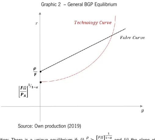
GRAPHIC 2 – GENERAL BGP EQUILIBRIUM 37
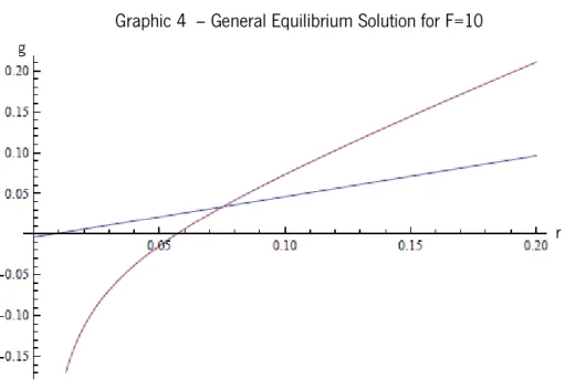
GRAPHIC 3 - GENERAL EQUILIBRIUM SOLUTION FOR F=5 38 GRAPHIC 4 – GENERAL EQUILIBRIUM SOLUTION FOR F=10 39 GRAPHIC 5 - GENERAL EQUILIBRIUM SOLUTION FOR F=20 39
8
1. Introduction
Financial development mainly refers to the size or efficiency of the financial system. The impact of financial development on economic growth is not a consensual topic among the economists. According to Levine (2005) the pioneers of modern economic growth theory didn’t approach financial aspects in their essays. For instance, the Nobel Laureate Robert Lucas (1988, p.6) described finance as an “over-stressed” determinant of economic growth and Joan Robinson (1952, p. 86) famously argued that "where enterprise leads finance follows."
Levine (1999) becomes a major seminal reference in finance and growth. The author argues that financial development can impact the level of growth by facilitating and improving the allocation of resources, across space and time in an uncertain environment. According to Levine (1999), financial institutions and markets may arise to improve problems created by information and transaction frictions through different types and combinations motivating distinct financial contracts, markets and institutions. The strong and positive link between the financial system and long-run economic growth has since been studied by a growing body of research which includes empirical analyses, on firm and industry-level studies, individual country-studies, time-series studies, panel-investigations, and broad cross-country comparisons (Levine, 2005).
It is observed that some models of economic growth show that financial instruments, markets, and institutions may mitigate the effects of information and transaction costs. The acquisition of information enables the increase of the intensity with which creditors exert corporate control, the provision of risk-reducing arrangements, pooling of capital, making transactions between agents and banks easier (Levine, 1999). Hence, we assume that financial development pushes the emergence of banks and consequently improves the acquisition of information. The availability of information enables an efficient allocation of credit, and financial contracts increase the confident of investors in receiving their money back.
Financial systems may also influence saving rates, investment decisions, technological innovation, and consequently long-run growth rates. According to Levine (2005), there is a growing group of researchers that examine how the financial development can affect de economic growth, including the research agenda that examines aspects as direct laws, regulations, and macroeconomic policies that shape financial sector operations. There is also a second research agenda that studies the political, cultural, and even geographic context influencing financial development.
9
A variety of academic literature has been produced about these topics in recent years, however, there are still many points unanswered and existing macroeconomic models generally have not yet created a direct relationship between finance and growth.
Considering this background and the importance of financial development to economic growth, here we will focus on the relationship between financial development and economic growth through the introduction of the component of financial intermediation in an existing growth model. Our paper is motivated by a research movement in macroeconomics towards understanding, through models of economic growth, how financial development can impact the rate of economic growth.
We start with a brief review of the main existing economic growth studies, after which we establish a relationship between existing theory and empirical research, explaining endogenous growth models based on R&D sector, mainly Thompson (2008a) model, which is based in previous models like Romer (1990), Rivera-Batiz and Romer (1991) and Evans el al (1998). Then, we discuss the main measures of financial development and how it can impact differently countries’ economies according to their economic characteristics.
Finally, seeking to establish theoretically a relationship between financial development and economic growth, we explore and model the inclusion of financial development in Thompson (2008a) model with internal investments costs, substituting this component for external investment cost, and introducing an analytical function for the price of patents. Additionally, we introduce financial development in the consumers’ side of the economy.
2. Objectives
In our dissertation, we start by presenting a literature review on endogenous growth theories and empirical studies about the relationship between financial development and economic growth. We also present a discussion about the main variables used to measure the financial development degree of one country.
These references support our main objective, which is to develop a new model demonstrating the relationship between financial development and growth. We’ll build on Thompson’s (2008a) analytical approach, replacing the internal cost of investment for an external cost of investment, with an analytical function for patents price which considering the influence of financial development.
We intend to find and demonstrate analytically a positive relationship between financial development and growth. We hope to show the relevance of our work not only for providing additional and hopefully more precise insights of the finance-growth relationship, but also for providing
policy-10
makers with further analytical tools for understanding the mechanisms through which finance contributes to economic growth
3. Literature Review
3.1 Economic Growth Models
Throughout this chapter we wish to describe the main characteristics of economic growth models and how the theories have changed over the years, pointing out the main authors in each current of growth research. We’ll describe the time line developed by Higachi (1998) which begins with the new classic theory, followed by the neoclassic theories, the neo-Schumpeterian and ends up with the new evolutionist view.
Other authors prefer to categorise the growth models differently from the above referred, considering also different models. According to Carvalho and Oreiro (2008), growth models are divided into first and second generation models. The first one contemplates the works of Domar (1946), Kalecki (1954), Kaldor (1956, 1957), Pasinetti (1962) and Robinson (1962), who believe that economic growth is based on the functional income distribution and implicitly in a full utilization of productive capacity. In this generation of growth models, the financial system and the use of paper money is neutral to the economy in the long-run. This notion is also valid for the second generation of models, Goodwin (1967), Rowthorn (1981), Dutt (1984, 1994), Bhaduri e Marglin (1990) and Lima (1999). The main difference between the first and the second generation is that the second one incorporates increased complex dynamics based on non-linear influences between the variables. In these models, there is flexibility in the degree of utilization of productive capacity and technological progress becomes endogenous. However, these models do not consider the role of finance in the accumulation of capital.
11
1Image 1 – Economic Growth Models According to Carvalho and Oreiro (2008)
Search: Own production (2019).
Higachi’s (1998) approach is illustrated in Image 2, which begins with the New-Classic theory from the 1970s, inspired by the classical principles of macroeconomic of general perfect equilibrium.
Search: Own production (2019).
The first main contributor is Robert Lucas who developed a methodological approach, considering substantive rationality, balance, demonstration methods and risk. Lucas' models are based on microeconomic dynamics (profit and utility maximization) and economic fundamentals. The conception of Lucas models is based in the general economic equilibrium which is conceived as a stationary stochastic process. In other words, economic phenomena are manifestations of the general economic equilibrium. Lucas considers the assumptions of maximization of utility and of profits in an environment
12
characterised by competitive equilibria and rational expectations, based on two behavioural postulates, first that economic agents act in their own interest and second that there is no excess of supply and demand. According to Dosi and Nelson (1994), Lucas integrates microeconomic factors in the explanations and configuration of macroeconomic variables by supposing that they are an aggregate result of individual agents’ action, like families and firms.
According to Higachi (1998), the industrial revolution introduced new questions related with the change of the aggregate variables, like the permanent growth of per-capita income and labour productivity, and new economic agents’ behaviour ideas, for firms and technology. A new theory or growth model capable of explaining these new regularities associated with the aggregate variables, innovation and microeconomic competition was necessary.
The neoclassical theory emerged to answer these new questions through the formulation of a macroeconomic analysis with solid micro-foundations: the neoclassical growth theory, which can be divided in three different categories according to the modelling technique. The traditional neoclassic models; first generation endogenous growth models; and second generation endogenous growth models.
The neoclassical traditional models are based on the hypothesis that declining marginal returns on capital eventually leads to the interruption of growth and to convergence between rich and poor countries. Thus, in this view, in order to sustain positive per-capita growth, it is necessary that the marginal productivity of capital is kept above the effective depreciation of capital per-capita thus keeping marginal returns to capital increasing or constant.
Following the traditional neoclassic model, come the endogenous growth models known as the Solow-Swan models. The new endogenous research-based growth theories consider economic growth as an endogenous result of one economic system based on technological progress, rather than being the result of external variables (Romer,1994).
The new neoclassical endogenous growth theories expanded in two additional different directions. One stream is based on linear models that consider a broad kind of capital (including various forms of capital) accumulation as the source of growth (The 𝑌 = 𝐴𝐾 Model). The second direction whose models consider human capital as the main source of growth. The first human-capital accumulation model was developed by Lucas (1988). According to Thompson (2008b) it was built on Solow’s model and introduced an equation for human capital accumulation, which allows for endogenous growth. Lucas model delivers the prediction that economic growth increases with the effectiveness of investment in human capital accumulation.
13
The innovation-based models are fathered by the horizontal-differentiation Romer’s (1990) model and by the neo-Shumpeterian vertical-differentiation Aghion and Howitt’s (1993) model, for whom innovation is induced by profit-seeking private firms and is the main engine of economic growth (Romer, 1994). Innovation in this case is a result of one R&D sector which needs specific resources to develop new technology. There is a right to use this new technology and it will be acquired by the manufacturing/intermediate goods sector who pay an amount of forgone output to the research sector. According to Higachi (2008), two different sub-classes of innovation based models can be distinguished: the variety of products or horizontal-differentiation and the quality of products or vertical-differentiation.
The variety of products view considers that the products are aggregated with the old ones in the production function. Such is the case of Romer's Model (1990), which then considers that the growth of the capital stock is related to the growth of intermediary goods in quantities, through the increasing availability of these intermediaries’ there's more production methods available resulting in an increase in productivity and then economic growth.
The second type of R&D models – the neo-shumpeterian models – are based on the idea that new designs with better quality replace the old designs. Aghion and Howitt’s (1993) model is the first one of this line based on creative destruction. In this model, the technological process is manifested through an increase in the productivity of the intermediates goods which produce the final good, in other words, the source of economic growth happens through innovations which are improvements of the intermediate goods’ productivity.
Through this new perspective, combined with Schumpeter (1943) ideas of endogenous innovation in economic growth theories, emerged a new evolutionist literature, which according to Higachi (1998) started in the 80s with Nelson and Winter (1982). These evolutionists models follow the neoclassical theory in placing innovation at the core of the growth, but diverge in some points such as the agents’ behaviour. They are based on the comprehension of the dynamic process of changes. The main objective is to create a theory of the economic dynamics of long-run, where there is uncertainty, rejecting the equilibrium method and adopting the non-equilibrium. These models adopt the economic phenomena as an evolutionary process and use behaviour grounds (Dosi and Nelson, 1994).
3.2 Economic Growth and Financial Development: Theoretical and Empirical models
The relationship between the financial system and economic growth has been studied since Schumpeter (1911) who argued that economic growth depends of financial market sophistication. For
14
Schumpeter, the level of development of financial intermediation importantly determines the rate of economic growth by affecting the pace of productivity growth and technological change.
According to Damasceno (2008), the inclusion of the financial system in the logic of productive system starts with Schumpeter and also Keynes who consider that there is complementarity between paper money and economic development. However, while for Schumpeter money influences the economy through the concepts of circular flow and economic development, Keynes argues that the existence of money neutrality or non-neutrality depends on whether we have a cooperative economy or a business economy. In both approaches money affects the long-run path of accumulation and the levels of capital and output.
Neoclassical theory also contributes to this topic, mainly through Solow’s (1956) model, in which economic growth is based on an exogenous variable and there is a limit to product growth, denominated as “steady-state” where the product growth is equal to the rate of population growth. When Solow introduces technological progress, in the “steady-state” the product growth depends both on the population growth and technological progress rates.
The importance of the relationship between finance and growth grew with the appearance of works based on endogenous growth, the starting point for the debate and literature on this subject. The idea that currency is endogenous is introduced in the post-Keynesian models like Dutt and Amadeo (1993) and Lima and Meirelles (2003). They assume that banks can effort additional demand of currency through the same interest rate which varies over time.
The influence of the financial system on the process of capital accumulation is based on a Schumpeterian inspiration where the process of technological innovation creates a greater demand for credit, which allows oligopolistic banks to increase their mark ups on the basic interest rate (which varies according to monetary policy), thus influencing the distribution of income and accumulation of capital in the economy.
Latest models introduce some new points, Evans et al (1998) create a model named “Growth Cycles” in which the economy switches stochastically between periods of low and high growth due to expectations regarding the interest rate. In their model, economy has a single state variable and the preferences and technology are homogeneous, resulting in the fact that opportunities in the economy are the same except for a scale factor determined by the state variable. The result of this model is that in the long-run the expectations determine whether the equilibrium of the economy is one of high-growth or of low-high-growth. According to Evans et al (1998) model, a continuum of equilibria approaching
15
a single steady state can offer a novel strategy for justifying the stickiness of prices and the power of monetary policy.
According to Morales (2001), classical references of this research area are Greenwood and Jovanovic (1990), Bencivenga and Smith (1991, 1993), Levine (1991, 1992) and Saint Paul (1992). These papers use the basic linear 𝑌 = 𝐴𝐾 framework combined with credit market models of financial intermediation. Here, financial-market institutions provide services of risk pooling and information about borrowers. Another responsibility of the financial sector is to facilitate the flow of resources from savers to investors in the presence of market imperfections.
Aghion, Howitt and Mayer-Foulkes (2005) suggest that financial development can accelerate convergence to steady state without changing the growth rate in the steady state. Their empirical study is based on a cross-section regression similar to Levine, Loayza and Back (2000) they add a term which represents the interaction between the initial relative GDP per-capita and the indicators of financial development, and find agreeing results with such hypothesis.
Following Howitt and Aghion (1998) and Aghion, Howitt and Mayer-Foulkes (2005), Morales (2001) introduces a specification for the contractual relationship between the researcher and the provider of funds for the research project in a model of endogenous technological change where there’s creative destruction. In her model, financial intermediaries are endowed with a monitoring technology that allows them to demand that researchers exert a higher level of effort than the one they would choose in the absence of monitoring and thus induces a higher research intensity that raises the economic growth rate. This model of research productivity reveals two external effects of opposite sign. On the other hand, the increase in R&D productivity will raise the arrival rate of innovations and on the other hand consequently raise the probability of an incumbent producer being driven out by the latest innovator.
Others famous references in economic growth models involving the financial sector are Saint-Paul (1992) and Bencivenga and Smith (1992). The work of Saint-Paul shows the relationship between financial market and the technological choice and how it impacts in the rate of real economic growth. The model shows the existence of a multiple equilibria, one equilibrium with the presence of financial market and another one without this one. The results show that costs of transacting in a financial market influence the choice of technology, implying the fact that economies with high transaction costs will rely on lower levels of technology production, which economize on financial market activity; this cause a long gestation use of this technologies and reductions on the real return on savings, hence limiting new investments. When the reductions in transactions costs are large enough, long maturity
16
capital investments with greater productivity tend to increase, then the capital market improvements are growth enhancing.
Bencivenga and Smith (1992) discuss the consequences of credit rationing in an endogenous growth model. Through a model where young generations are divided between lenders and borrowers, this relationship is established through contracts and there’s an adverse selection problem in credit markets in distinguishing between high and low-quality investments. The credit rationing functions are, in this model, a mechanism for sorting owners according to the quality of investments. In the equilibrium, the growth rate and the level of credit rationing are determined jointly, and it’s a relation of loan profits and the rental rate of capital. The discussion about the solution shows that credit rationing conditions the loan quantities and the interest rates hence policy actions that reduce it would be welcome.
Galetovic (1996) also models the relationship between financial intermediation and growth, adding the degree of a researcher’s specialization. In this model creditors can verify the outcome of a research firm before spending units of labor, in other words, they can check how healthy the company is before investing their money. The research firms’ specialization is characterized by the number of employees working in the company, which influence production and consequently output. In this model the output of research firms carries probabilities of success. The results show that intermediaries will emerge according to the specialization of the research firms, because a coalition of firms will decrease monitoring costs that are not negligible relative to the size of the loan and thus the credit market will be dominated by a large intermediary.
Differently from Galetovic (1996), Blackburn and Hung (1998) introduce financial intermediation by the investor households, which through a saving channel (the financial institutions) provide more efficient and lower cost investment than through a direct loan. The equilibrium of the model shows that growth occurs through an increasing variety of intermediate goods associated with an increasing number of firms engaged in research and development, resulting in an increasing number of projects that in turn generates the possibility of diversification by the intermediaries and increases the intensity of competitive demand for human capital.
One other example of model connecting financial intermediation with economic growth is Harrison et al (1999). This model works with the idea that financial intermediation amplifies productivity and output growth, but also that economic growth increases the number of banks due to the increase of activities and projects, driven by the cost savings relative to regional specialization. This model includes
17
additional variables such as the distance between banks and research firms and the density of capital and labor.
King and Levine (1993), De la Fuente and Marín (1996) and Blackburn and Hung (1998) introduce informational frictions in the credit market, providing a rationale for the appearance of financial intermediaries (Morales, 2001).
Overall, up to this point, “theory strongly suggests that financial intermediaries play an important role in researching productive technologies before investment and in monitoring managers and projects after channeling capital to those projects.” (Levine, 1997)
Empirically speaking, according to King and Levine (1993), the level of financial intermediation becomes a good predictor of economic growth, even after controlling for many other country specific characteristics. Through both pure cross-country instrumental variables procedures and dynamic panel techniques, Levine et al. (2000) find a positive relationship between the level of financial-intermediation development and long-run economic growth, which is not due to simultaneity bias.
Nevertheless, one shortcoming of these empirical analyses is that financial-intermediation development may be a leading indicator of economic growth, but not an underlying cause of economic growth. Still, according to Beck et al (2000), economies with better-developed financial intermediaries grow faster, enjoy faster rates of productivity growth, experience more rapid capital accumulation, and have higher savings rates.
This happens because of the fact that financial intermediation generates lower costs of investment in research, through exerting corporate control; managing risk; mobilizing savings; and conducting exchanges. By providing these services to the economy, financial intermediaries influence savings and allocation decisions in ways that may influence positively long-run growth rates (Beck et al, 2000).
Levine (2005) includes innovation in his model and defends that financial institutions provide firms useful information for innovation, increasing innovation activities. Levine defines relationships between: (i) financial-market development and innovation; (ii) innovation and economic growth; and (iii) financial development and economic growth.
Levine (2005) also emphasizes that we do not have yet adequate theories on why different financial structures emerge or why financial structures change. Differences in legal tradition (La Porta et al. 1997) and differences in national resource endowments that produce different political and institutional structures (Engerman & Sokoloff, 1997) might be incorporated into future models of financial development.
18
Empirically, Levine (1999) uses the legal determinants of banking development as instrumental variables for financial intermediation indicators to control for simultaneity bias. A positive impact of financial development on economic growth is not found, but it is found that the exogenous component of financial development is strongly related with per-capita income growth, productivity improvement and capital formation. Controversially, in other study, Levine et al. (2000), using generalized methods of moments (GMM) estimators, find strong evidence of financial development affecting economic growth positively. Later, Easterly and Levine (2005) conclude that countries with developed financial systems tend to experience faster economic growth than those with poorly developed financial systems. Such faster economic growth appears as a result of higher productivity and higher per-capita income. Although many studies suggest a positive relationship between financial development and economic growth, Singh (1997) argues that financial development may not be beneficial for economic growth. Firstly, the volatility of the stock market pricing process in developing countries makes it a poor guide to efficient investment allocation. Secondly, interactions between stock markets and currency markets can create economic shocks and exacerbate macroeconomic instability, and consequently reduce long-run growth. De Gregorio and Guidotti (1995) also find a negative impact of financial development on the Latin American economic growth.
3.3 Financial Development measurements
An important point of scientific discussion is the measurement of financial development. The performance of banks and of the stock market are the most common variables used to measure the financial system development, the main point being the existence of different measures of banking and stock market development.
Levine and Zervos (1998) use liquidity indicators as a measure of financial development, such as the turnover ratio to study the stock market impact on economic growth, their results are consistent with the view that stock market liquidity facilitates long-run growth and suggest that stock markets provide different financial functions from those provided by banks.
In order to measure the level of financial development, specifically, the functioning of the financial system, King and Levine (1993) use the degree of central bank versus commercial banks in allocating credit. The performance of nonbanking institutions is also added as a measure of the functioning of financial system and has been debated by the researchers. As mentioned before, King and Levine (1993) also include in their analysis the size of financial intermediaries which is equal to the liquid liabilities of the financial system, including currency plus demand and interest-bearing liabilities of
19
banks and nonbanking financial intermediaries. They find a strong and positive relationship between these financial-development indicators and three economic growth indicators: long-run real per-capita growth rates, capital accumulation; and productivity growth.
The link between other economic variables and financial development also has been debated in previous related studies. McKinnon-Shaw (1973) links the level of financial intermediation to the real interest rate, explaining that a positive real interest rate stimulates financial savings and financial intermediation, increasing the supply of credit to the private sector, which in turn stimulates investment and growth. However, De Gregorio (1995) disagrees with this view, classifying interest rate as a poor indicator of financial intermediation and defending that high interest rates may indeed have a negative impact on investment and economic growth through credit rationing, increasing product costs, international debt, and domestic finance problems.
De Gregorio (1995) hypothesizes that a monetized economy reflects a highly developed capital market and should be positively related to growth performance. Considering that financial markets have two main functions, credit allocation and liquidity providing, he believes that investment and growth depend on well-functioning financial markets. The author uses the ratio of domestic credit to the private sector as a proxy of the degree of financial-intermediation development to analyze his hypothesis.
We also need to consider that the impact of financial development on the rate of economic growth can vary across countries, as the response to different variables depends on country-specific structural factors as well as on country-specific economic circumstances. Each country’s income level is differently affected by the financial system. In fact, Aghion, Howitt and Mayer-Foulkes (2005) and Rioja and Valev (2004) show that the effects of finance on growth vary according to one country’s income level.
According to Rioja and Valev (2004), the strong contribution of financial development to productivity, which will in turn affect positively the economic growth rate, does not occur until a country has reached a certain threshold-income level. Until the economy has reached such threshold-income level, financial development will influence the economic growth through capital accumulation.
Other factors, not associated with income, can also explain the divergence across national financial systems, for instance: (i) inflation; (ii) research financing costs; (iii) historical factors such as, for example, a prolonged depression (Gurley and Shaw ,1967); (iv) government restrictions on the banking system, such as an interest rate ceiling and high reserve requirements, which can complicate financial development and reduce output growth (Christopoulos and Tsionas, 2004); (v) the law, and the
20
functioning of the courts and processes of litigation between debtors and creditors (Gurley and Shaw, 1967).
Besides, the high finance-income ratios accumulate only throughout considerably long periods of social evolution, and such accumulation occurs at different rates across countries. These factors show that financial development may influence the economic growth differently according to each country’s characteristics.
Concluding, we can see that there is an important debate and research on finance and growth, which allows us to confront all theories and create new ones to contribute to the literature on financial development and economic growth. The influence of one country’s specific characteristics on the relationship between finance and growth is perceived but not completely identifiable or measurable. Hence, the present dissertation will focus on the factors that can be captured analytically and generalized into a growth model with finance.
4. Methodology/Model
We propose to contribute to the theoretical literature on finance and growth, by developing a new endogenous growth model with financial intermediation and with it analyze theoretically the relationship between financial development and economic growth. We will extend Thompson’s (2008a) model in order to introduce price of a patent for intermediate good, in other words, an analytical function for the price of designs/patents, such that it depends on financial intermediation.
We wish to show analytically that financial intermediation has a positive impact on the economic growth rate and also wish to illustrate such influence through a numerical solutions exercise.
4.1 Specification and results of the model
We will build on Thompson’s (2008a) model. This model uses the application of Hayashi’s (1982) internal cost of investment framework to a continuous time context. According to Thompson (2008a) other authors like Benavie et al (1996), Cohen (1993) and Van Der Ploeg (1996) have also used Hayashi’s costly investment in AK-type of models. Differently, this model introduces the internal investments costs into a one-sector R&D-based growth model. Thompson (2008a) uses Rivera-Batiz and Romer (1991) to specify a one-sector framework, where both consumption and total capital are produced with the same technology. The model additionally assumes that intermediate goods are complementary to each other in the production function, in other words, an increase in the demand
21
for one intermediate good will also increase the production of all the other intermediate goods. Thompson (2008a) uses Evans et al. (1998) complementarities specification.
The model developed by Rivera-Batiz and Romer (1991) is part of the R&D-based models, where innovation and consequently technological progress are determined endogenously. In Romer's (1990) model technological progress is endogenous due the introduction of researchers and their ideas as a product, intermediate good firms, and their profit-seeking behavior. Based on new developments of the industry, like consumer electronics, computers and pharmaceuticals, Romer (1990) incorporates the efforts and the importance of the R&D to developing new technologies, and integrates the imperfect competition rationale in order to introduce economic rewards to R&D activities. Romer’s model advances in new economic growth theory considering that technological progress is a result of the firm’s search for profits in a context where technology is treated as non-rival but excludable. Rivera-Batiz and Romer’s (1991) is an evolution from the first model created by Romer, this new model presents the R&D sector in two different ways, first as knowledge-driven and then the lab equipment specification. Thompson (2008a) builds on these of this first generation of R&D models in order to develop a one-sector growth model with costly investment and complementarities.
4.2 Thompson Model (2008)
The setting is a closed economy inhabited by identical immortal individuals. On the preferences side of the decentralized model, homogeneous consumers maximize the discounted value of their utility (1), subject to a budget restriction (2):
𝑀𝑎𝑥 ∫ 𝑒−𝜌𝑡𝑈(𝐶𝑡)𝑑𝑡 ∞ 0 , 𝑈(𝐶𝑡) = 𝐶𝑡1−𝜎 1−𝜎 (1) 𝐵𝑡̇ = 𝑟𝐵𝑡+ 𝑤𝑡+ 𝐶𝑡 (2) As usual, 𝐶𝑡 is consumption at date 𝑡 and 𝜌 is the discount rate of consumption, 𝜎(> 0) is the inverse of the intertemporal elasticity of substitution between consumption at two periods of time. Variable 𝐵𝑡 represents assets, 𝑤𝑡 the salary and 𝑟 is the interest rate.
Solving the representative consumer’s inter-temporal optimization problem, we find that the representative consumer facing a constant interest rate 𝑟 chooses to have consumption growing at the constant rate 𝑔𝑐 which is demonstrated through the Euler equation (3):
𝑔𝑐 =𝐶̇
𝐶 =
1
𝜎(𝑟 − 𝜌) (3)
On the production side, there are three productive activities: final good production, intermediate goods production and the R&D sector, responsible for the invention of new designs for new intermediate
22
goods. Based on Evans et al. (1998), there is complementarity between intermediate goods in the production function, the final good production function is (4):
𝑌(𝑡) = 𝐿(𝑡)1−𝛼(∫ 𝑥
𝑖(𝑡)𝛶𝑑𝑖
𝐴(𝑡)
0 )𝜙, 𝜙 > 1, 𝛶𝜙 = 𝛼 (4)
where, the final good 𝑌 is produced using as inputs labor 𝐿, which is assumed as a constant value, and 𝐴 differentiated durable intermediate goods 𝑖, each produced in quantity 𝑥𝑖.
Parameter 𝜙 is assumed to be greater than one so that intermediate goods are complementary, that is increasing the quantity of one intermediate good also increases the marginal productivity of the other goods. Restriction 𝛶𝜙 = 𝛼 is assumed in order to maintain homogeneity of degree one of the production function.
Parameter restriction (5) is imposed in order to solve the model for a constant growth rate:
ξ =𝜙−1
1−𝛼 (5)
In the intermediate goods sector there is production of physical machines for each of existent invented intermediate goods. Equation (6) shows the relation between capital 𝐾 and the intermediate goods, assuming that it is used one unit of physical capital to produce one unit of each intermediate good:
𝐾(𝑡) = ∫ 𝑥𝑖(𝑡)𝑑𝑖 𝐴(𝑡)
0
The third productive sector, the R&D, is modelled considering Rivera-Batiz and Romer (1991), where new designs are invented with the same technology as the that of the final good and of intermediate goods.
Following Rivera-Batiz and Romer’s (1991) lab equipment specification, final output, intermediate goods and new inventions are all produced under the same technology. In Rivera-Batiz and Romer’s (1991) one-sector economy, total output can be expressed by (7):
𝑌 = 𝐶 + 𝐾̇ +𝐴̇
𝑍 = 𝐻
𝛼𝐿𝛽∫ 𝑥(𝑖)𝐴 1−𝛼−𝛽𝑑𝑖
0 (7)
The model's symmetry implies that 𝑥(𝑖) = 𝑥(𝑗) for all 𝑖 and 𝑗 less than 𝐴, the reduced-form expression for total output in terms of 𝐻, 𝐾, 𝐿, and 𝐴 is according to (8).
𝑌 = 𝐶 + 𝐾̇ +𝐴̇
𝑍 = 𝐻
𝛼𝐿𝛽𝐴(𝐾/𝐴)1−𝛼−𝛽 (8)
= 𝐻𝛼𝐿𝛽𝐴𝐾1−𝛼−𝛽𝐴𝛼+𝛽
The result is that in the lab equipment model, output of new designs has the same homogenous of one degree production function as the manufacturing sector and they depends only on the aggregate
23
stocks of inputs, not on their allocation between the two sectors. The price of physical capital is equal to 1 and the price of each new invention is equal to 1/𝑍.
Thompson (2008a) assumes that each invention has a price equal to 𝑃𝐴𝑖ξ units of forgone output,
where 𝑃𝐴 represents the fixed price of one new design in units of forgone output and 𝑖ξ represents an
additional cost of patent 𝑖 in terms of foregone output. In other words, this represents a higher cost of production designs with a higher index with the purpose of avoiding explosive growth. Hence, total investment in each period is given by:
𝑊̇(𝑡) = 𝐾̇(𝑡) + 𝑃𝐴𝐴̇(𝑡)𝐴(𝑡)ξ, (9)
where 𝐾̇(𝑡) represents investment in physical capital, and 𝑃𝐴𝐴̇(𝑡)𝐴(𝑡)ξ represents investiment in
innovation of new designs. Total capital 𝑊(𝑡) and its accumulation accordingly equations (10) and (11):
𝑊(𝑡) = 𝐾(𝑡) + 𝑃𝐴𝐴(𝑡)ξ+1
ξ+1 (10)
𝑊̇(𝑡) = 𝑌(𝑡) − 𝐶(𝑡) (11)
The producers of final goods sector are price takers in the market of intermediate goods. Thus, in equilibrium the rental rate paid for each intermediate good will be equal to its marginal product, which means that the demand curve for each intermediate good producer is:
𝑅𝑗(𝑡) = 𝜙𝛶𝐿1−𝛼𝑥
𝑗(𝑡)𝛾−1(∫ 𝑥𝑖(𝑡)𝛾𝑑𝑖)𝜙−1
𝐴(𝑡)
0 (12)
The symmetry of the model implies that 𝑅𝑗(𝑡) = 𝑅(𝑡), and 𝑥𝑗(𝑡) = 𝑥(𝑡), which means that the production function for aggregate output can be rewritten according to (13).
𝑌 = 𝐿𝐴1+ξ(𝛼
𝑅)
𝛼
1−𝛼 = 𝐵𝑊, (13)
where 𝐵 represents the constant marginal productivity of total capital.
In the usual R&D-based growth models firms face zero capital accumulation costs and determine their optimal level of capital stock according to investment rate which can’t be determined. As they cannot determinate the investment level, firms maximizes their present discounted value of cash flows subject to their costs of investment.
According to Hayashi’s (1982), investment requires an additional installment cost. The following equations (14) and (15) show the amounts required of new units of capital and the installation cost function respectively.
𝐽(𝑡) = 𝐼(𝑡) + 1 2⁄ 𝜃𝐼(𝑡)2
𝐾(𝑡) (14)
𝐶(𝐼(𝑡), 𝐾(𝑡)) = 1 2⁄ 𝜃𝐼(𝑡)2
24
Through these equations the maximization problem for the firms is: 𝐻(𝑡) = 𝐹(𝐾(𝑡), 𝐿̅) − 𝐼(𝑡) − 1 2⁄ 𝐼(𝑡)2
𝐾(𝑡) + 𝑞(𝑡)(𝐼(𝑡) − 𝐾̇(𝑡)),
where 𝑞(𝑡) is the market value of capital. It is assumed zero capital depreciation. Considering that installing 𝐼(𝑡) = 𝑊̇(𝑡) new units of total capital, the transversality condition of this optimization problem is lim
𝑡→∞𝑒
−𝑟𝑡𝑞(𝑡)𝑊(𝑡) = 0.
Following the growth rate of output is 𝑔 = 𝐼⁄ , the first-order condition is equal to 𝑞 = 1 + 𝜃𝑔. 𝑊 The co-state equation is equivalent to:
𝑞̇ 𝑞 = 𝑟 − 𝐵 +1 2𝜃𝑔 2 𝑞
The problem is solved for its balanced growth path solution, which implies that 𝑞 must be constant, hence equation (16) can be re-written as:
𝑞 =𝐵 +
1
2𝜃𝑔
2
𝑟
The intermediate goods sector production decisions will be based on the maximization of the monopolist profits according to equation (17). It is assumed that to produce one physical unit of an intermediate good it is needed one unit of capital.
𝑚𝑎𝑥 𝜋𝑗(𝑡)𝑥𝑗(𝑡) = 𝑅𝑗(𝑡)𝑥𝑗(𝑡) − 𝑟𝑞𝑥𝑗(𝑡), (17) which leads to the markup rule:
𝑅𝑗 =𝑟𝑞 𝛶
Following the logic of this model, a new firm wishing to enter in this market to produce the 𝐴𝑡ℎ
intermediate good, needs to spend up-front an amount, which is equal to a fixed constant price in units of forgone output equivalent 𝑃𝐴 plus an additional coefficient which represents the extra cost of this new higher indexed patent in terms of foregone output 𝑖ξ. Hence, equation (18) represents the new
intertemporal zero profit condition.
𝑃𝐴𝐴(𝑡)ξ= ∫ 𝑒−𝑟(𝜏−𝑡)𝜋 𝑗(𝜏)𝑑𝜏 ∞
𝑡 , (18)
which assuming no bubbles is equivalent to:
ξ𝑔𝐴 = 𝑟 − 𝜋 𝑃𝐴𝐴ξ
In the balanced growth path, 𝑥 grows at the rate ξ𝑔𝐴 and the output 𝑦 grows at the rate (1 + ξ)𝑔𝐴. Rearranging the profits equation (19) we find another expression for the growth rate (19) which we name Technology curve as did Rivera-Batiz and Romer (1991):
25 𝜋 = (1−𝛶 𝛶 ) 𝑟𝑞𝐿𝐴 ξ(𝛼𝛶 𝑟𝑞) 1 1−𝛼 , (19) 𝑔 =1+ξ ξ [𝑟 − Ω (𝑟𝑞) 𝛼 1−𝛼 ] , Ω =( 1−𝛾 𝛾 )𝐿(𝛼𝛾) 1 1−𝛼 𝑃𝐴 (20)
Through equation (11) we can assume that a constant growth rate of total capital implies that consumption grows at the same rate as output, which means that, as labor is constant the per-capita economic growth rate is given by:
𝑔𝐶 = 𝑔𝑦 = 𝑔𝑘 = 𝑔𝑤 = 𝑔 = (1 + ξ)𝑔𝐴
The general solution of this model is obtained solving the system, which is a result of equations (3) and (19), considering 𝑞 = 1 + 𝜃𝑔: 𝑔 =1 𝜎(𝑟 − 𝜌) 𝑔 =1 + ξ ξ [𝑟 − Ω (𝑟 + 𝑟𝜃𝑔)1−𝛼𝛼 ] , 𝑟 > 𝑔 > 0, where, Ω =( 1−𝛾 𝛾 )𝐿(𝛼𝛾) 1 1−𝛼 𝑃𝐴 .
The restriction, 𝑟 > 𝑔 > 0 is imposed so that present values will be finite, and also so that our solution(s) have positive values for the interest rate and the growth rate. While the Euler equation is linear and positively sloped in the space (𝑟, 𝑔), the Technology curve is nonlinear, in other words, the Technology curve does not allow for the analytical derivation of the equilibrium solution, in Thompson (2008a) the solving of the system is made through a numerical example.
4.3 Thompson Model (2008) and Financial Intermediation of Research
The purpose of this section is to introduce financial intermediation through the price of acquiring patents by intermediators sector, extending Thompson’s (2008a) model by removing internal costs of investment, and by introducing an analytical function for the price of designs/patents, which depends on financial intermediation. We will propose that there is a positive relationship between the degree of financial development and economic growth.
1.1.1 Production Side
Considering Thompson (2008a) and Evans et al. (1998), the production side is divided in three sectors: the final good producers, the intermediate producers and the research sector, which produces
26
the patents. The model we build, also assume the existence of complementarities between intermediate goods in the aggregate (final good) production function:
𝑌 = 𝐿1−𝛼(∫ 𝑥𝑖𝛶𝑑𝑖 𝐴
0 )
𝜙, 𝜙 > 1, 𝛶𝜙 = 𝛼,
where, 𝑌 is the final good, produced using inputs of labour 𝐿, a number 𝐴 of differentiated durables intermediate goods 𝑖, each produced in quantity 𝑥𝑖 and 𝐾 = ∫ 𝑥𝑖(𝑡)𝛶𝑑𝑖
𝐴
0 .
It is also considered in this economy that 𝐿 is constant; and the parameter restriction ξ =𝜙−1
1−𝛼 ,
hence (1 + ξ) =𝜙−𝛼
1−𝛼. The restriction 𝛶𝜙 = 𝛼 is imposed in order to preserve the function
homogeneity degree one and 𝜙 > 1 represents that intermediate goods are complementary one to another.
1.1.2 Final good sector
The final good sector sells their output and set their work demand in a perfect and pure market competition. Therefore, the final good producers, wishing to maximize their profits choose a quantity of 𝐿𝑡 and 𝑥𝑖 in each 𝑡. According to the profits function (21), the final good producers acquire each intermediate good according to maximization rule:
𝜋𝑌= 𝑃𝑌𝑌 − 𝑤𝐿 − 𝑅0𝑥0− 𝑅1𝑥1− ⋯ − 𝑅𝐴𝑥𝐴 (21)
𝑑𝜋𝑌 𝑑𝑥𝑖 = 0,
where 𝑃𝑌 is the price of the final good, assumed as 𝑃𝑌 = 1; 𝑅 is the price to rent each intermediate good 𝑥 and 𝑤 is the salary.
The first maximization conditions is:
𝑑𝜋𝑌 𝑑𝐿 = 0
This one is not necessary in this model, because 𝐿 only works in one sector, so there is no need for a labour market equilibrium.
Considering the perfect market competition the price will be equal to the marginal productivity, that is, the marginal cost.
𝑑𝜋𝑌 𝑑𝑥0 = 0 ⇔ 𝑑𝜋𝑌 𝑑𝑥0 = 𝑅0 𝑑𝜋𝑌 𝑑𝑥1 = 0 ⇔ 𝑑𝜋𝑌 𝑑𝑥1 = 𝑅1 ⋮
27 𝑑𝜋𝑌 𝑑𝑥𝐴 = 0 ⇔ 𝑑𝜋𝑌 𝑑𝑥𝐴 = 𝑅𝐴 Generalizing: 𝑑𝜋𝑌 𝑑𝑥𝑖 = 0 ⇔ 𝑑𝜋𝑌 𝑑𝑥𝑖 = 𝑅𝑖 So, 𝑅𝑖 = 𝑑𝑌 𝑑𝑥𝑖= 𝜙𝛶𝑥 𝛶−1𝐿1−𝛼(∫ 𝑥 𝑖𝛶𝑑𝑖 𝐴 0 ) 𝜙−1 (22) This equation represents the price paid by the final goods sector for the intermediate firms to rent the intermediate goods, it is directly related with the level of technology 𝐴 and the complementarities between intermediate goods 𝜙.
1.1.3 Intermediate goods sector
The producers of intermediate goods are the intermediate producers, each one produces one-unit variety and operate in a monopolistic competition market, in function of patents acquired for each producer. The intermediate goods firms buy these patents to produce new intermediate goods and then, they sell it to the final good sector.
In every period of time, there are agents deciding whether to become intermediate good producers or not. If one wants to become an intermediate good producer, then one must buy upfront (in the period of becoming an intermediate firm), the patent for producing the intermediate good. In other words, in this model, in order to produce an intermediate good, one firms needs to by the patent for it. To by the patent, they need long-term credit because they reap the benefits of selling intermediates in the future, while they pay for physical capital today, so we propose that the price of the patent is related with the financial development.
We assume that the price of a patent for intermediate good 𝑖 is equal to: Ƥ = 𝑃𝐴
𝐹 𝑖
ξ (23)
where, 𝑃𝐴 is the fixed price of each patent, 𝐹 is the parameter that represents Financial Development and 𝑖ξ is an additional cost meaning that the higher number of patents in existence, the higher the
cost of inventing one more patent.
Regarding Financial Development, we assume that an increase in 𝐹 results in a decrease in Ƥ, in other words, the higher the level of financial development the lower the cost of a patent.
28
This assumption is supported by studies like Tadesse (2005) which analyzed the relationship between financial development and technology innovation, where technological innovations are partly attributable to availability of capital, thus leading to reduction in costs of innovation.
Financial development may reduce theses costs of research through the raise of capital, contributing to real cost reduction. Financial development also may improve savings and capital mobilization, increasing the supply of capital for investment, that is, the lower innovation costs can be related to lower transaction costs and improvement of liquidity, accompanied by the improvement of capacity for mobilizing large capital. Other factor is that financial development reduces problems of informational asymmetry.
Therefore, the study concludes that financial development can reduce the real costs and result in higher technological progress. Based on these points we consider that a reduction in real costs also imply lower patent prices.
If one becomes an intermediate firm, one must pay upfront the patent’s price and then one becomes the exclusive producer of one intermediate good. That is, it has from that moment onwards, monopolistic profits in each period of time, from that moment until infinity. In other words, the decision to produce a new intermediate good depends on the comparison between the discounted stream of net future revenues, and the cost Ƥ of investing in a design, which has to be paid in the moment the producer acquires it, before profits earns.
Thus, the decision to become an intermediate good firm is described by the following equation: 𝑃𝐴 𝐹 𝐴 ξ = ∫ 𝑒−𝑟(𝜏−𝑡)𝜋 𝑖(𝜏)𝑑𝜏 𝜏=∞ 𝜏=𝑡
at 𝑡, one becomes an intermediate firm and buys patent 𝐴 (the latest), meaning that the cost of becoming one intermediate good firm must be equal to the present value of all the monopolistic profits 𝜋, from 𝜏 = 𝑡 up to 𝜏 = ∞.
The following equation represents the zero-profit-condition for all periods of time: 𝑃𝐴 𝐹 𝐴 ξ = 𝜋 𝑖(𝑡) + 𝜋𝑖(𝑡 + 1) 𝑒𝑟 + 𝜋𝑖(𝑡 + 2) 𝑒2𝑟 + 𝜋𝑖(𝑡 + 3) 𝑒3𝑟 + ⋯
Differentiating it in order to time, we get an equivalent zero-profit condition that must hold in each period of time: (𝑃𝐴 𝐹 𝐴ξ) ̇ =𝑃𝐴 𝐹 𝐴 ξ𝑟 − 𝜋 𝑖,
29 𝑃𝐴 𝐹 ξ𝐴̇𝐴 ξ−1 = 𝑃𝐴 𝐹 𝐴 ξ𝑟 − 𝜋 𝑖 ⇔ ξ𝐴̇ 𝐴= 𝑟 − 𝜋𝑖 𝑃𝐴 𝐹 𝐴 ξ ⇔ 𝑔𝐴 =1 ξ[𝑟 − 𝜋𝑖 𝑃𝐴 𝐹𝐴ξ ] (24)
Considering their elasticity demand curve and marginal costs constant, the monopolistic competitor solves his problem by charging a monopoly price, which is a mark-up over marginal cost, so considering the monopolistic profits 𝜋𝑖, it must maximize, in each period, this profits:
𝜋𝑖 = 𝑅𝑖𝑥𝑖− 𝑟𝑥𝑖 (25) where 𝑟 is the cost of using physical capital and it is assumed that each unit of each intermediate good requires the use of one unit of physical capital, 𝐾. Then,
𝜋𝑖 = 𝛼𝑥𝑖𝛾−1𝐿1−𝛼(∫ 𝑥 𝑖 𝛾 𝑑𝑖 𝐴 0 ) 𝜙−1 𝑥𝑖− 𝑟𝑥𝑖 The profit maximization condition is the following:
𝑑𝜋𝑖 𝑑𝑥𝑖 = 0 ⇔ 𝛾𝛼𝑥𝑖𝛾−1𝐿1−𝛼(∫ 𝑥 𝑖 𝛾 𝑑𝑖 𝐴 0 ) 𝜙−1 − 𝑟 = 0 ⇔ 𝑅𝑖 = 𝑟 𝛾 (26)
This equation represents the mark-up rule, which says that the intermediate good price is higher than marginal cost because we are in a monopolistic competition environment, where 𝑟 is the marginal cost. The idea is that a firm incurs a fixed cost when it produces a new intermediate good and recovers this cost by selling its good for a price 𝑅𝑖 higher than its constant marginal cost.
𝑅𝑖 = 𝑟 𝛾> 𝑟 The model enjoys the property of symmetry meaning that: 𝑅𝑖 is equal for all 𝑖
𝑥𝑖 is equal for all 𝑖
𝜋𝑖 is equal for all 𝑖
This property allows us to simplify our expressions:
𝑅𝑖 = 𝑅 = 𝑟 𝛾
30
Wherefore, first, all intermediate goods are sold for the same price. 𝑥𝑖 = 𝑥
Second, all the intermediate goods are produced in the same quantities 𝜋𝑖 = 𝜋,
and thirdly, all the intermediate firms have the same profits. Hence:
𝑅 = 𝛼𝐿1−𝛼𝑥𝛾−1𝐴𝜙−1𝑥𝛾𝜙−𝛾
⇔ 𝑅 = 𝛼𝐿1−𝛼𝐴𝜙−1𝑥𝛼−1
⇔ 𝑅 = 𝑟
𝛾 (27)
Reconsidering the profits equation:
𝜋 = 𝑅𝑥 − 𝑟𝑥 = 𝑅𝑥 − 𝛾𝑅𝑥 = (1 − 𝛾)𝑅𝑥 = (1 − 𝛾)𝛼𝐿1−𝛼𝐴𝜙−1𝑥𝛼 ⇔ π = (1 − 𝛾)𝛼𝐿1−𝛼𝐴𝜙−1𝑥𝛼 (28) Following, 𝑅 = 𝛼𝐿1−𝛼𝐴𝜙−1𝑥𝛼−1 ⇔ 𝑥𝛼−1 = 𝑅 𝛼𝐿1−𝛼𝐴𝜙−1 ⇔ 𝑥1−𝛼 =𝛼𝐿 1−𝛼𝐴𝜙−1 𝑅 ⇔ 𝑥 = 𝐿𝐴ξ[𝛼 𝑅] (1 1−𝛼⁄ ) ⇔ 𝑥 =𝐿𝐴 ξ(𝛾𝛼)(1 1−𝛼⁄ ) 𝑟(1 1−𝛼⁄ )
Hence, substituting the value of 𝑥 in the profits equation (28):
π = (1 − 𝛾)𝛼𝐿1−𝛼𝐴𝜙−1[𝐿𝐴 ξ𝛾(1 1−𝛼⁄ )𝛼(1 1−𝛼⁄ ) 𝑟(1 1−𝛼⁄ ) ] π =(1 − 𝛾)𝐿𝛼𝛼(𝛼 1−𝛼 ⁄ ) 𝛾(𝛼 1−𝛼⁄ )𝐴𝜙−1+𝛼ξ 𝑟(𝛼 1−𝛼⁄ ) π =(1 − 𝛾) 𝛾(𝛼 1−𝛼 ⁄ )𝐿𝛼(1 1−𝛼⁄ )𝐴ξ 𝑟(𝛼 1−𝛼⁄ ) (29) (30)
31
Through these equations, we have that:
𝑔𝐴 =1
ξ[𝑟 −
𝜋
(𝑃𝐴⁄ )𝐴𝐹 ξ],
which is equivalent to:
𝑔𝐴 =1 ξ[𝑟 − (1−𝛾)𝛾(𝛼 1−𝛼⁄ )𝐿𝛼(1 1−𝛼⁄ )𝐴ξ 𝑟(𝛼 1−𝛼⁄ ) (𝑃𝐴⁄ )𝐴𝐹 ξ ] ⇔ 𝑔𝐴 = 1 ξ[𝑟 − 𝛺𝐴ξ 𝑟(𝛼 1−𝛼⁄ ) 𝐹 𝑃𝐴𝐴ξ] ⇔ 𝑔𝐴 = 1 ξ[𝑟 − 𝐹𝛺 𝑃𝐴𝑟(𝛼 1−𝛼⁄ )] where 𝛺 = (1 − 𝛾)𝛾(1 1−𝛼⁄ )𝐿𝛼(1 1−𝛼⁄ ).
Now, we will solve the problem for the Balanced Growth Path (BGP) solution. As we will see later and following Thompson (20008a) model, the Euler Equation says that a BGP solution requires that the interest rate 𝑟 is constant. A constant interest rate implies that 𝑅 = 𝑟 𝛾⁄ is also constant. Besides that, we have the following assumptions:
𝐿 is assumed constant 𝑃𝐴 is assumed constant 𝐹 is assumed constant Considering this, we have:
𝑥 = 𝐿𝐴ξ[𝛼 𝑅] 1 1−𝛼 ⁄ ⇔ 𝑔𝑥 = ξ𝑔𝐴
Remembering as mentioned before, 𝑅 = 𝛼𝐿1−𝛼𝐴𝜙−1𝑥𝛼−1 and 𝑅 = 𝑟 𝛾, so:
𝑔𝑅 = (𝜙 − 1)𝑔𝐴+ (𝛼 − 1)𝑔𝑥 = 0
⇔ 𝑔𝑥 = (1 − 𝜙 1 − 𝛼) 𝑔 ⇔ 𝑔𝑥 = ξ𝑔𝐴
Through the profit equation (30) we can find the growth profits rate as:
π =(1 − 𝛾) 𝛾(𝛼 1−𝛼
⁄ )𝐿𝛼(1 1−𝛼⁄ )𝐴ξ
𝑟(𝛼 1−𝛼⁄ )
⇔ 𝑔𝜋 = ξ𝑔𝐴 The symmetry of the model also means that:
𝑌 = 𝐿1−𝛼(𝑥𝛼+ 𝑥𝛼+ ⋯ + 𝑥𝛼)𝜙
32
where 𝑥𝛼 is added 𝐴 times.
Considering the aggregate production function, we have the following growth rates: 𝑌 = 𝐿1−𝛼𝐴𝜙𝑥𝛼
⇔𝑔𝑌 = 𝜙𝑔𝐴+ 𝛼𝑔𝑥 ⇔ 𝑔𝑌 = 𝜙𝑔𝐴+ 𝛼ξ𝑔𝐴
⇔ 𝑔𝑌 = (𝜙 + 𝛼ξ)𝑔𝐴 ⇔ 𝑔𝑌 = (1 + ξ)𝑔𝐴
Additionally, the physical capital is equal to 𝐴 times the values of 𝑥, according to equation (32) 𝐾 = 𝑥 + 𝑥 + ⋯ + 𝑥
⇔ 𝐾 = 𝐴𝑥 (32) So, the growth rate of 𝐾 is:
𝑔𝐾 = 𝑔𝐴+ ξ𝑔𝑥 ⇔ 𝑔𝐾 = (1 + ξ)𝑔𝐴 This means that equation (31) can be rewritten as:
𝑔𝑌 =1 + ξ ξ [𝑟 −
𝐹𝛺
𝑃𝐴𝑟(𝛼 1−𝛼⁄ )]
with 𝛺 = (1 − 𝛾)𝛾(1 1−𝛼⁄ )𝐿𝛼(1 1−𝛼⁄ )
This equation (33) is our Technology equation.
1.1.4 Consumption Side
Following Thompson (2008a) it is considered a closed economy inhabited by identical immortal individuals. Homogeneous consumers maximize the discounted value of their consumption utility, subject to their budget restriction. We assume that Financial Development also influences households’ decisions. The Financial Development degree, designated by 𝐹, makes households more prone to save. Hence, we specify consumers inter temporal problem as:
𝑀𝑎𝑥 ∫ 𝑒𝜌 𝐹⁄ 𝑈(𝐶 𝑡)𝑑𝑡 ∞ 0 , 𝑈(𝐶𝑡) = 𝐶𝑡1−𝜎 1−𝜎 𝐵𝑡̇ = 𝑟𝐵𝑡+ 𝑤𝑡+ 𝐶𝑡
As usual, 𝐶𝑡 is consumption at date 𝑡 and 𝜌 is the discount rate of consumption, 𝜎 (> 0) is the
inverse of the intertemporal elasticity of substitution between consumption at two periods. Variable 𝐵𝑡 represents assets, 𝑤𝑡 the salary and 𝑟 is the interest rate. The discount rate is, we assume, equal to 𝜌 𝐹⁄ with 𝜌 being the traditional rate of time reference and 𝐹 is the degree of Financial Development.
33
The consumers wish to maximize their utility of consumption during their lifetime. Therefore, the current value Hamiltonian and the maximization conditions are:
𝐻𝑡= 𝐶𝑡 1−𝜎 1 − 𝜎+ 𝜃𝑡[𝑟𝐵𝑡+ 𝑤𝑡− 𝐶𝑡] 𝑑𝐻 𝑑𝐶 = 0 𝑑𝐻 𝑑𝐵 = 𝜌𝜃 − 𝜃̇
Solving these two conditions, we find that the representative consumer facing a constant interest rate 𝑟 chooses to have consumption growing at the constant rate 𝑔𝑐, which is demonstrated through the familiar Euler equation:
𝑔𝑐 =𝐶̇ 𝐶 = 1 𝜎(𝑟 − 𝜌 𝐹) (34)
Equation (34) describes the consumer’s decisions between consumption and savings in long-run equilibrium. For example, if the interest rate increases, savings increase, hence consumption growth also increases. Through Graphic1 it is possible to analyse the behaviour of our proposed Euler Equation.
Search: Own production (2019).
Analyzing the other variables, we have the following results:
If the rate of 𝜎 increases, consumers prefer to consume now and consumption will increase too, consequently the consumption growth rate (𝑔𝑐) will decrease.
34
If the interest rate 𝑟 increase, consumers will prefer to save their money, increasing the family savings 𝑆𝐹, and the consumption will decrease, consequently the consumption growth rate (𝑔𝑐) will increase.
If the rate of time preference 𝜌 increases, it means that consumers are more impatient to buy, increasing the present consumption and decreasing the consumption growth rate (𝑔𝐶).
Considering the financial development 𝐹, if it increases we have that families will save more money, increasing savings 𝑆𝐹, consequently the present consumption will decrease and the consumption growth rate (𝑔𝐶) will increase.
Chin and Ito (2005), through a model that controls for institutional factors, sought to explain the determinants of the current account budgets of the governments with the goal to inform the recent debate over the source of and solution to the global savings glut. In their regressions, they also estimated the relationship between the financial development and the national savings. Their results show that for the countries considered in the less developed countries (LDC) and emerging market group (EMG) groups, higher levels of financial development results in higher levels of savings. In spite of the results being different for industrialized countries, this finding supports our premise that higher financial development propels individuals to save more.
1.1.5 General Equilibrium
Seeking to solve the model, first, we need to find the general equilibrium. Primarily, we need to show that 𝑔𝐶 = 𝑔𝑌. It’s known that:
𝑔𝐾 = 𝑔𝑌 = (1 + ξ)𝑔𝐴
Then, we can use the economy’s budget constraint: 𝐾̇ = 𝑌 − 𝐶,
which says that capital accumulation is equal to investment (assuming zero capital depreciation), and it is also equal to savings, and consequently is equal to what is left of output after consumption.
𝐾̇ = 𝐼 = 𝑆 = 𝑌 − 𝐶 Then, let us divide 𝐾̇ = 𝑌 − 𝐶 by 𝐾
𝐾̇ 𝐾= 𝑌 𝐾− 𝐶 𝐾 ⇔ 𝑔𝐾 = 𝑌 𝐾− 𝐶 𝐾
35
Considering the fact that the BGP solution requires constant growth rates, the capital growth rate (𝑔𝐾) is constant, so: 𝑔𝐾̇ = 0 ⇔ (𝑌 𝐾) ̇ = (𝐶 𝐾) ̇ ⇔ 𝑔𝐶 = 𝑔𝐾 = 𝑔𝑌 That is, a constant 𝑔𝐾 requires that time-variation of ratio 𝑌
𝐾 is equal to time-variation of 𝐶
𝐾.
We have shown earlier that: 𝑔𝐶 = 𝑔𝐾 = 𝑔𝑌 = (1 + ξ)𝑔𝐴. So, we can find the general equilibrium by solving the system:
𝑔 = 1 𝜎(𝑟 − 𝜌 𝐹) 𝑔 =1 + ξ ξ [𝑟 − 𝐹𝛺 𝑃𝐴𝑟(𝛼 1−𝛼⁄ )] with 𝛺 = (1 − 𝛾)𝛾(1 1−𝛼⁄ )𝐿𝛼(1 1−𝛼⁄ )
Hence, we can solve for the general equilibrium BGP solution by solving the system of two equations, in two unknowns, 𝑔 and 𝑟. Our two equations are the linear Euler Equation (34) and the Technology Equation (33). As (33) which is non-linear, it is necessary to find information about this curve’s inclination. We use the Implicit Function Theorem as a tool to assist us in this study:
Given 𝐹(𝑟, 𝑔) = 0, then: 𝑑𝑟 𝑑𝑔= − 𝑑𝐹 𝑑𝑔 𝑑𝐹 𝑑𝑟 So, 𝑔 =1 + ξ ξ [𝑟 − 𝐹𝛺 𝑃𝐴𝑟(𝛼 1−𝛼⁄ )] with 𝛺 > 0 ⇔ ξ𝑔 = (1 + ξ)𝑟 −(1 + ξ)𝐹𝛺 𝑃𝐴𝑟(𝛼 1−𝛼⁄ ) ⇔ F(𝑟, 𝑔) = ξ𝑔 − (1 + ξ)𝑟 +(1 + ξ)𝐹𝛺 𝑃𝐴𝑟(𝛼 1−𝛼⁄ ) = 0 𝑑𝐹 𝑑𝑔 = ξ 𝑑𝐹 𝑑𝑟 = −(1 + ξ) − (1 + ξ)𝐹𝛺 ( 𝛼 1−𝛼) 𝑃𝐴𝑟 2𝛼−1 1−𝛼 𝑃𝐴2𝑟1−𝛼2𝛼