Volatility of returns, variations in prices and volume traded: evidence from the main stocks in Brazil

Electronic copy available at: http://ssrn.com/abstract=1435309

Volatility of returns, variations in prices and volume traded: evidence from the main stocks in

Brazil

Cesar Nazareno Caselani

cesar.caselani@fgv.br

William Eid Junior

william.eid@fgvsp.br

2005

Key words

stock price determinants, Brazil

Abstract:

We study the relationship between the volatility and the price of stocks and the impact that variables such as past volatility, financial gearing, interest rates, stock return and turnover have on the present volatility of these securities. The results show the persistent behavior of volatility and the relationship between interest rate and volatility. The results also showed that a reduction in stock prices are associated with an increase in volatility. Finally we found a greater trading volume tends to increase the volatility.

1. Introduction

Studies related to the dynamic of stock markets have been of great importance in financial literature. Issues related to the spreading of information between investors, the volume traded and the volatility of returns are relevant aspects when it comes to understanding better the behavior of these assets.

Electronic copy available at: http://ssrn.com/abstract=1435309

A stock market has depth if at a given moment in time, there are purchase and sell orders both above and below the price at which a certain stock is being traded. When a security is traded in a deep market temporary imbalances in the buy (sell) orders are immediately compensated for by sell (buy) orders, thereby avoiding the occurrence of substantial variations in price and any consequent instability in the quotations. The immediate communication of the quotations of the assets and the immediate execution of the orders are pre-conditions for a market to present depth.

The breadth of a market is seen if there is a large volume of buy and sell orders. Therefore a market needs to show a good degree of liquidity, as measured by the trade volume, before it can be considered to be broad. Generally speaking financial analysts believe that the price trend in a broad stock market is more significant and longer-lasting. For the analysts the highs and lows of a particular stock are more trustworthy when accompanied by the security being traded in large volume. A particular market may present depth without being broad. While depth demands only the existence of orders above and below the current quotation of a security, breadth needs a large trading volume with a particular security before it can be seen.

The third desirable attribute of a market – resiliency - has to do with the capacity of the market to adjust to price variations that arise as a result of momentary imbalances in buy and sell orders. The faster investors can acquire information about prices and past transactions with the assets the more depth, breadth and resiliency the market has.

The above attributes suggest that the volume and the price at which a stock is traded reflect a natural signal of the prospects for the security. The publication of information to investors is strongly related to the frequency of the trades and the volume traded. In turn the frequency of trades and the volume involved in the transactions are variables that are representative of the level of liquidity achieved by a particular stock. When a security is frequently traded investors receive a steady flow of new information. If the agents set a price for the stock at a level that is too high, market transactions involving the asset will help them recognize this fact. The same is true if a stock is under-priced. The quantity of buy and sell orders provides investors with information about variations in the equilibrium price of a given asset. When a stock is rarely traded the quality of information that can be gleaned from the orders is low and investors are not sure about the appropriate price equilibrium level. In principle, the greater the frequency with which a stock is traded the more informed the investor will be about the “fair price” for it.

the assets, therefore, constitute important variables when it comes to understanding the dynamic of the stock market, as represented by a group of stocks that are traded, especially those that are traded most frequently.

In this study the dynamic of the Brazilian stock market is explored from the point of view of the behavior of a group of stocks that were frequently present in the Sao Paulo Stock Exchange Index (Ibovespa) in the period between 1995 and 2003. Using the sample we study the possible factors that determine the behavior of securities. The predictability of the behavior of a stock is related to the volatility of the asset’s return. If the volatility of stock returns follows a logic that can be foreseen then it is possible to estimate the variation in the price of the security. Obviously the possibility of producing an estimate of the behavior of a stock reflects the fact that markets are not fully efficient. Various works have been developed with the idea of producing an explanation for the behavior of the volatility of stock returns. Among the approaches existing on volatility behavior three will be developed in this study: the gearing theory (Christie, 1982), the volatility feedback theory (Pindyck, 1984) and the divergence of opinion between economic agents model (Hong and Stein, 2003). According to Lo and Wang (2000), the price and traded volume of assets are fundamental building blocks when it comes to constructing any theory about the interaction of agents in the market.

The above ideas serve as the basis for the overall objective of this study, which is to explain the price behavior of the main stocks traded on the Sao Paulo Stock Exchange between 1995 and 2003. By means of economic approaches that seek to understand the behavior of the volatility of stock returns the econometric tests in this work aim to contribute by providing new results on the market for equities in Brazil.

The topics in this study are structured in the following way: Topic 2 gives the theoretical basis of the work; Topic 3 gives the methodology employed; Topic 4 gives the empirical results of the study and Topic 5 presents the conclusions.

2. Theoretical basis

In the theoretical basis presented below we have tried to follow a well-defined logic. Therefore we present three approaches that try to throw light on the causes for the behavior of the volatility of stock returns. In order they are the gearing theory, the feedback theory and the divergence of opinion between economic agents model.

2.1. The effects of gearing on the volatility of stock returns

According to the theory of gearing one of the factors that can affect the price volatility of a specific stock is the company’s degree of financial gearing. The seminal ideas on this theory are present in the articles of Black (1976) and Christie (1982). In an influential article on the relationship between the price of stocks and volatility of their returns Christie (1982) comments that the relationship between the variance in returns and the price of a stock tends to be negative. The “gearing effect” that the theory deals with claims that a drop in the price of a stock (negative return) increases the financial gearing of the company to the extent that it changes the proportion of the capital of third parties in relation to own capital. With a greater degree of indebtedness the stock becomes more risky, which brings about an increase in the volatility of its subsequent returns. According to the author the arrival of information in the market is responsible for part of the fluctuations seen in the variance of the returns on these assets.

In his article Christie (1982) tested three hypotheses regarding the volatility of stock returns. The first is that the volatility of a stock’s return is an increasing function of the degree of financial gearing. The second is that the relationship between the volatility of a stock’s return and the financial gearing of the company is sufficient to induce negative elasticity between this volatility and the value of the stock. The third hypothesis has to do with the impact of the rates of interest on the volatility of stock returns; as the impact may be positive or negative, empirical tests need to be carried out.

To formalize the negative relationship between stock volatility and the level of financial gearing Christie (1982) starts with the equation

(1)

where σ represents the standard deviation of the stock’s return and LR = D/S, with LR being the degree of financial gearing of the stock, t is time, V is the market value of the company, D is the volume of third party capital and S is the market value of the company’s own capital. This being the case the volatility of the stock’s return (σS) is an increasing positive function

of the financial gearing and the elasticity (θS) of the volatility of return in relation to the price of the stock is provided by

)

1

(

,t V t

S

=

σ

+

LR

σ

S

S

S S

∂

∂

⋅

=

σ

However, it is known that

so

and this means that

therefore,

(2)

With regard to the empirical tests estimates of the elasticity θS, that relate the volatility of return to the price of the

stock, can be initially obtained using the following regression

(3)

While the above regression can be used to obtain the elasticity θS of the stocks, it does not help us determine the

relationship between the volatility of a stock’s return and the degree of financial gearing of the company. To do so it is necessary to work with the specification

(4) where QR is the quotient between third party capital and own capital. From the above specification we can expect that the coefficient β1 will be positive and significant, suggesting that the volatility of a stock’s return is an increasing function of

S

D

S

D

LR

σ

σ

σ

σ

σ

=

(

1

+

)

=

1

+

=

+

2

S

D

S

σ

σ

−

=

∂

∂

)

1

(

)

1

(

=

−

+

−

⋅

+

=

∂

∂

⋅

LR

LR

S

D

LR

S

S

S

σ

σ

σ

σ

)

1

(

+

−

=

LR

LR

θ

−

1

≤

θ

≤

0

t t t S t S t S

u

S

S

+

+

=

−1 1

, ,

ln

ln

α

θ

σ

σ

t t t

S,

=

β

+

β

QR

+

w

the degree of financial gearing. Relating equations 3 and 4, we can expect that a significant relationship between the volatility of the stock’s return and the financial gearing of the company is sufficient to induce negative elasticity between this volatility and the value of the stock.

Finally the model that includes also the rate of interest (r) as a determinant of the volatility of the stock’s return is given by

(5) The results of the study of Christie (1982) point to a negative relationship between price and the volatility of a stock’s return. This relationship is attributed to the financial gearing of the company. The study specifically shows that the volatility of stock returns is an increasing function of financial gearing and that this fact causes a negative relationship between the elasticity of the volatility of a stock’s return and its price. As far as the rate of interest is concerned the author discovered a positive relationship between it and the volatility of a stock’s return. This result is consistent with the fact that the value of a company decreases with an increase in the rate of interest. With a reduction in the value of the company the participation of debt in relation to own capital increases thereby causing an increase in the degree of financial gearing. In turn greater financial gearing brings about greater volatility in the returns on a stock.

2.2. Return volatility and risk premium

In addition to the gearing on the volatility of the returns of a particular stock there are arguments in literature that uphold that stock returns exhibit asymmetric volatility; in other words the volatility trend increases at times of negative returns. One explanation for this is the volatility feedback theory found in the works of Pindyck (1984), Campbell and Hentschel (1992) and Bekaert and Wu (2000).

According to Campbell and Hentschel (1992) possible changes in the volatility of stock returns create important effects on the return demanded by investors and therefore on the price levels and the volatility of the returns on stocks. While the theory of gearing maintains that variations in the price of a stock are the cause of the swings in the volatility of the returns on the security, the volatility feedback theory defends the opposite idea, in other words that it is the variation in the volatility of the returns that causes changes in stock prices. According to the volatility feedback theory an expected increase in the volatility of a stock’s return increases the return demanded by the stockholder (an increase in premium because of the risk), leading to a fall in the price of the asset. According to this theory volatility behavior is related to the new information that reaches the market. The theory of volatility feedback also works with the idea that the volatility of

t t t t

S,

=

β

+

β

QR

+

β

r

+

w

stock returns is persistent and the occurrence of new facts related to a company, whether they are positive or negative, increases both present and future volatility.

For example if positive news is published about the payment of dividends by a certain company this news tends to be followed by other information about the company, thereby adding to the volume of new information about it. An increase in the volume of information tends to increase the volatility of a stock’s return, which causes an increase in the rate of return demanded by the stockholders and reduces the price of the stock, thereby reducing the positive impact of the news about the dividends. A further possible scenario is one in which there is bad news about the payment of dividends. In this case the publication of new information would equally increase the volatility of the stock’s return and reduce its price. However, in the bad news scenario the increase in the volatility of returns would amplify the negative impact of the information, creating even more negative returns for the stock.

In short, if the news is positive the effect of the good news is partially compensated for by an increase in the volatility of stock returns. Therefore an increase in the price of the securities is hindered by the growing risk that an upward movement will be followed by a drop in prices. On the other hand when a large amount of negative information occurs the effect of the news is accompanied by an increase in the volatility of a stock’s return, thereby increasing even more the negative effect of the information flow. Campbell and Hentschel (1992) argue that the result of this process of persistent volatility creates a distribution of returns with negative asymmetry. Going further, it is possible to identify the existence of an “asymmetric volatility” of returns, with a tendency for an increase in volatility as a result of the negative returns on a stock.

The negative asymmetry of stock returns found by Campbell and Hentschel (1992) was based on the weighted return of the CRSP stock index. In the work of Duffee (1995), on the other hand, positive asymmetry prevailed in the case of stocks that were looked at individually. According to the author one of the possibilities for the difference between the distribution of returns for individual stock and for aggregated indices is related to the behavior of a factor that is common to all stocks. This common factor might present a distribution with negative asymmetry, such that this result would define the result for the aggregate returns of the stocks included in the index. In the case of individual stocks, however, idiosyncratic returns might represent a distribution with positive symmetry. Duffee (1995) arrives at this conclusion after observing that the returns of the individual stocks that were part of his sample showed positive asymmetric distributions.

The intuition behind the equilibrium model with divergence of opinion comes from the article written by Miller (1977). In this article the author argues that the price of assets will reflect a more optimistic assessment if pessimistic investors stay out of the market. In Miller’s (1977) model optimistic investors keep their stocks because they imagine that they are going to go up in value. These investors, however, suffer losses because the best estimate for the price of a stock is the average opinion of the market. The result is that the bigger the disagreement about the “fair price” for a stock, the greater will be the difference between the market price of the stock and its equilibrium value, with the future return of the security being less.

Unlike the upward movement in stock prices forecast by Miller (1977), in the model of Hong and Stein (2003) this movement is eliminated. The reason for this is the existence in Hong and Stein’s model of perfectly rational arbitrators. These arbitrators would act in the sense of eliminating any pricing that is out of equilibrium.

Hong and Stein’s (2003) equilibrium model was developed in an attempt to explain sharp swings in stock prices and the possible contagion of a stock as a result of the movement in another security. One of assumptions of the model is that negative stock returns are more pronounced after periods with a large volume of trades. In this case the volume traded represents the intensity of the disagreement between investors. More specifically the authors seek to throw light on the reason for the abrupt drop in stock prices, taking into consideration the asymmetry of information between the investors. According to Ofek and Richardson (2003), today there is a growing body of literature that looks to associate the heterogeneous expectations of investors to movements in stock prices.

Hong and Stein (2003) start with the assumption that there are two investors, A and B. Both investors have private indications (prospects) with regard to the variation of a stock in a particular period of time. Even though the indications of the two investors contain useful information investor A pays attention only to his indication, thus ignoring possible revelations made to the market by investor B. This over-confidence on the part of investor A as far as his own indication is concerned leads inexorably to divergence of opinion about the behavior of the stock. This difference of opinion leads in turn to negative asymmetry in the returns produced by the stock. Negative asymmetry means that the distribution of the stock’s return tends to present a greater probability of negative returns than of positive ones.

investor A and the arbitrators. The arbitrators are sufficiently rational to imagine that B’s sign is lower than A’s sign, but they have no way of knowing by how much. Therefore the market price of the stock at moment 1 reflects A’s information but does not succeed in fully incorporating B’s information.

After moment 1 has passed at moment 2 investor A receives a positive sign. In this case A continues being the more optimistic of the two investors and he incorporates the new indication to the stock price. The indication that investor B received at moment 1 is still unknown by the market. If instead of receiving a positive indication investor A receives a negative indication at moment 2 then the information received by B at moment 1 may come to light. This happens because investor A interrupts his purchase of stock. Investor B, on the other hand, waits until the drop in the stock price is compatible with the indication he received at moment 1. In other words the arbitrators wait for the moment in which investor B begins to buy stock. In this way B will be supplying information to the market that he received at moment 1.

Hong and Stein (2003) argue that when the divergence of opinion between investors A and B at moment 1 is pronounced B’s indication will tend to remain hidden thereby producing the negative asymmetry of returns at moment 2. Furthermore large divergence of opinion at moment 1 creates above normal volumes of trade, when investor A buys and the arbitrators sell the securities. Therefore the greater the volume traded at moment 1 the more negative will be the asymmetry at moment 2. The direct relationship between the volume traded and the negative asymmetry of stock returns is one of the most relevant assumptions in the authors’ model. In short the model relates the greater divergence of opinion between investors with sharper falls in stock prices and a greater volume traded, without new information necessarily being spread in the market.

There are significant differences between models like that of Hong and Stein (2003) and models of volatility feedback, like the one of Campbell and Hentschel (1992). While the former relate the volume traded to the intensity of the negative asymmetry in stock returns, in the latter the variable referring to the volume of trades is not explicitly mentioned. Another difference between the models has to do with the fact that the feedback theory works with a representative market agent structure and does not take into consideration the asymmetry of information between investors. Finally the volatility feedback model demands the existence of a large flow of news so that large price movements are generated. Hong and Stein’s model does not assume that such an intensity of new information is necessary for there to be price movements.

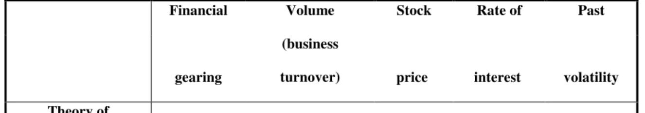
Table 1: The influence of explanatory variables on the volatility of stocks, according to the different theories.

Financial Volume Stock Rate of Past

gearing

(business

turnover) price interest volatility

Financial positive Does not apply negative positive

Does not apply

Gearing

Theory of positive with no

Volatility

Does not

apply Difference negative

Does not

apply Positive

feedback Of opinion

Equilibrium model positive with

With divergence

Does not

apply Difference negative

Does not

apply Positive

Of opinion Lagged volume

Chen, Hong and Stein (2001) related the divergence of opinion among investors to the negative asymmetry present in the distribution of returns of a group of stocks. The authors investigated the determining factors for the asymmetry in the stock returns using cross-sectional regressions to do so. The results they discovered are consistent with Hong and Stein’s (2003) model that forecast that negative asymmetries are more probable when there is large divergence of opinion between investors. In line with Hong and Stein (2003), the results of the study by Chen, Hong and Stein (2001) point to a greater negative asymmetry in the case of stock that has suffered an increase in traded volume in relation to the historical trend. Another conclusion was that stock with positive returns in previous months were more susceptible to negative asymmetry. Justification for this would be the existence of speculative bubbles.

To better understand the differences existing between the theories Table 1 summarizes the main aspects related to each one of the approaches previously mentioned.

3. Methodology

3.1. Sample

The sample in this study is made up of liquid stock present in the São Paulo Stock Exchange Index (Ibovespa) between 1995 and 2003. Liquid stocks are understood to be those that fulfill two basic requirements for being included in the sample. The first requirement is that the stock was being traded in the market in the year 2003. The second demand was that the stock had been included in Sao Paulo Stock Exchange’s theoretical portfolio on at least ten occasions during the period being studied. This sample was chosen due to the need for the stocks included to present minimum levels of liquidity that would allow for the quantitative tests to be carried out. There is no way of carrying out tests that relate volume and volatility using securities that are rarely traded. The sample included the period between January, 1995 and September, 2003. The daily data referring to the stock closing prices were taken from the Economática data base, as was information relating to the volume traded on each day (quantity of securities and the financial volume). In total 35 different stocks were taken into consideration.

The tests were carried out taking into consideration quarterly periods. In these tests we included the standard deviation of stock returns in the quarter, the amount of indebtedness at the end of quarter, the quarter-end rate of interest and the trading turnover for each stock. Seasonal influences were removed from the stock turnover series to avoid quarterly distortions, such as the absence of stagnation of the data. More details on the variables included in the study are presented below.

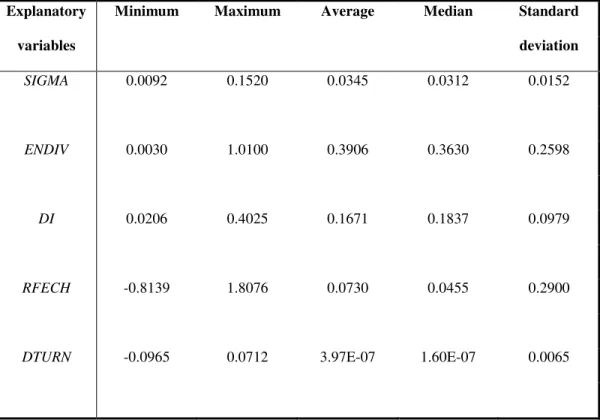
3.2. Description of the variables and descriptive statistics

Table 2 shows the descriptive statistics of the sample in quarterly periods. The SIGMA variable represents the quarterly standard deviation of stock returns. ENDIV is the level of indebtedness of the company at the end of the quarter. DI represents the inter-bank deposit rate at the end of each quarter. RFECH is the return on the stock during the quarter and

DTURN is the average turnover of trade with the security over the quarter, with the effects of seasonal influences removed.

The turnover of trade with the security is calculated by dividing the number of stocks of a particular company traded on any one day by the total number of the company’s stock in circulation. DTURN is given by

Table 2: Descriptive statistics of the sample.

Explanatory Minimum Maximum Average Median Standard

variables deviation

SIGMA 0.0092 0.1520 0.0345 0.0312 0.0152

ENDIV 0.0030 1.0100 0.3906 0.3630 0.2598

DI 0.0206 0.4025 0.1671 0.1837 0.0979

RFECH -0.8139 1.8076 0.0730 0.0455 0.2900

DTURN -0.0965 0.0712 3.97E-07 1.60E-07 0.0065

4. Empirical results

The results for the elasticity of the volatility of the returns in relation to the stock price, in accordance with equation 3 shown previously, appear in Tables 3 and 4. The specification used in both tables is

(7)

Where θS represents the elasticity of the volatility of returns in relation to the stock price and the variable LNRFECH

represents the logarithmic return of the security.

Table 3: Estimate by period of the elasticity of the volatility of returns in relation to the stock price.

Explanatory Period Period Period Sample

Variables 1995-1997 1998-2000 2001-2003 1995-2003

t t S

t

LNRFECH

u

Constant 0.063885 -0.032995 -0.021454 -0.001168 (2.45) ** (-1.86) *** (-1.97) ** (-0.11) LNRFECHt -0.543839 -0.225279 -0.224445 -0.300142

(-5.09) * (-3.86) * (-5.55) * (-7.90) *

R2 0.082 0.038 0.075 0.056

Adjusted R2 0.079 0.035 0.072 0.055

Durbin-Watson 2.407 2.467 2.746 2.583

Number of

observations 291 380 385 1056

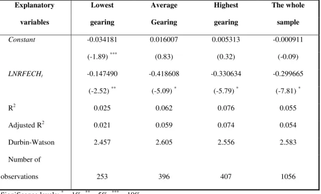
Table 4: Estimate by gearing level of the elasticity of the volatility of returns in relation to the stock price.

Explanatory Lowest Average Highest The whole

variables gearing Gearing gearing sample

Constant -0.034181 0.016007 0.005313 -0.000911

(-1.89) *** (0.83) (0.32) (-0.09)

LNRFECHt -0.147490 -0.418608 -0.330634 -0.299665

(-2.52) ** (-5.09) * (-5.79) * (-7.81) *

R2 0.025 0.062 0.076 0.055

Adjusted R2 0.021 0.059 0.074 0.054

Durbin-Watson 2.457 2.605 2.556 2.583

Number of

observations 253 396 407 1056

Significance levels: * = 1%, ** = 5%, *** = 10%.

From the results of the two tables it is possible to observe that the elasticity coefficient is to be found in the interval between -1 and zero. This occurred both in the division of the sample into three different periods (Table 3) as well as in the division by the degree of gearing of the companies (Table 4). This result confirms the behavior of the elasticity as forecast by Christie (1982); in other words there exists a negative relationship between volatility and stock price behaviors. A drop in the price of assets tends to cause an increase in the volatility of securities. Despite the fact that the results in Table 4 suggest some possibility that greater gearing results in more negative elasticity (companies with average and high gearing present more significant results than those with lower gearing) this sign is not conclusive. It is important to note that in both tables all the elasticity coefficients present significance levels of 1% (except in companies with lower gearing).

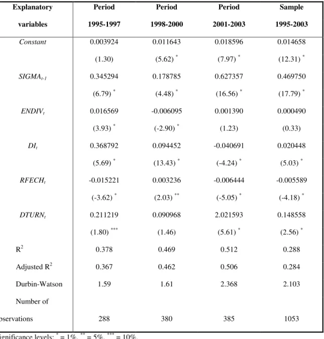
Table 5 shows the results generated by the influence of a set of explanatory variables on the behavior of the quarterly volatility of the stocks contained in the sample. As can be seen besides the results for the whole sample, Table 5 presents the results for the periods from 1995 to 1997, 1998 to 2000 and finally 2001 to 2003. The equation used in the table is

(8)

The results of Table 5 provide evidence of the persistent behavior of the volatility, thus corroborating the idea of volatility feedback. This can be seen in the positive and significant coefficient of the SIGMAt-1 variable. With regard to the

t t t

t t

t

t

SIGMA

ENDIV

DI

RFECH

DTURN

u

influence of financial gearing (ENDIV variable) on the volatility of stock returns the results are not conclusive. While the impact of indebtedness on return volatility is positive and significant in the period 1995 to 1997, between 1998 and 2000 it became negative and significant. In the period from 2001 until 2003 and for the whole of the sample the ENDIV coefficients are not significant. These inconclusive results corroborate the arguments of authors like Duffee (1995), who affirm that the degree of financial gearing of a company is not enough to explain the volatility of the returns on its stock. As far as the rate of interest variable (DI) is concerned, it presented a positive and significant relationship with the volatility of stock returns. This is the same result found by Christie (1982), who argues that an increase in the rate of interest reduces the value of companies, thereby increasing their gearing and consequently the volatility of stock returns. However, even though the results of Table 5 point to a positive relationship between the rate of interest and the volatility of stock returns, this fact cannot be justified by the gearing level of the companies.

Table 5: Cross-section estimate of stock returns (by period).

Explanatory Period Period Period Sample

variables 1995-1997 1998-2000 2001-2003 1995-2003

Constant 0.003924 0.011643 0.018596 0.014658

(1.30) (5.62) * (7.97) * (12.31) *

SIGMAt-1 0.345294 0.178785 0.627357 0.469750

(6.79) * (4.48) * (16.56) * (17.79) *

ENDIVt 0.016569 -0.006095 0.001390 0.000490

(3.93) * (-2.90) * (1.23) (0.33)

DIt 0.368792 0.094452 -0.040691 0.020448

(5.69) * (13.43) * (-4.24) * (5.03) *

RFECHt -0.015221 0.003236 -0.006444 -0.005589

(-3.62) * (2.03) ** (-5.05) * (-4.18) * DTURNt 0.211219 0.090968 2.021593 0.148558

(1.80) *** (1.46) (5.61) * (2.56) *

R2 0.378 0.469 0.512 0.288

Adjusted R2 0.367 0.462 0.506 0.284

Durbin-Watson 1.59 1.61 2.368 2.103

Number of

observations 288 380 385 1053

Significance levels: * = 1%, ** = 5%, *** = 10%.

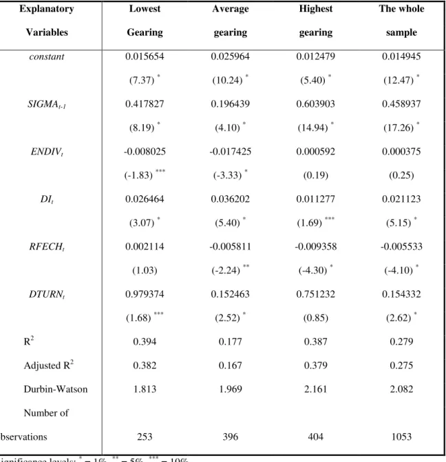
Table 6: Cross-section estimate of the volatility of stock returns (by level of gearing).

Explanatory Lowest Average Highest The whole

Variables Gearing gearing gearing sample

constant 0.015654 0.025964 0.012479 0.014945

(7.37) * (10.24) * (5.40) * (12.47) *

SIGMAt-1 0.417827 0.196439 0.603903 0.458937

(8.19) * (4.10) * (14.94) * (17.26) *

ENDIVt -0.008025 -0.017425 0.000592 0.000375

(-1.83) *** (-3.33) * (0.19) (0.25)

DIt 0.026464 0.036202 0.011277 0.021123

(3.07) * (5.40) * (1.69) *** (5.15) *

RFECHt 0.002114 -0.005811 -0.009358 -0.005533

(1.03) (-2.24) ** (-4.30) * (-4.10) *

DTURNt 0.979374 0.152463 0.751232 0.154332

(1.68) *** (2.52) * (0.85) (2.62) *

R2 0.394 0.177 0.387 0.279

Adjusted R2 0.382 0.167 0.379 0.275 Durbin-Watson 1.813 1.969 2.161 2.082 Number of

observations 253 396 404 1053

Significance levels: * = 1%, ** = 5%, *** = 10%.

5. Conclusions

company gearing. Therefore a drop in the price of the assets tends to cause an increase in the volatility of the securities. With regard to the link between company gearing and the volatility of stock returns the results were not conclusive.

The tests we carried out gave evidence of the persistent behavior of the volatility, thereby corroborating the idea of volatility feedback. As far as the rate of interest is concerned this had a positive and significant relationship with the volatility of stock returns. The results showed also that a reduction in stock price is associated with an increase in the volatility of return of the securities. This relationship is consistent with the theory; in other words, a drop in stock price is associated with a greater return demand by the stockholders and consequently with the perception of greater risk related to the security. Finally we found that a greater volume of trading tends to increase the volatility of stock returns. This result supports the argument of the theories of divergence of opinion among investors. The greater the volume traded, the greater is the amount of new information in the market, and the greater is the potential for divergence of opinion among those participating, thus causing greater volatility in stock returns.

Additional econometric tests are now necessary to interpret the results in more depth. However it is already possible to foresee some aspects of the behavior of stocks in the Brazilian market.

References

Bekaert, Geert e Wu, Guojun.Asymmetric volatility and risk in equity markets. Review of Financial Studies, v. 13, n. 1, p. 1-42, 2000.

Black, Fischer. Studies of stock price volatility changes. Proceedings of the 1976 meetings of the American Statistical Association, Business and Economics Statistics Section (American Statistical Association, Washington, DC), p. 177-181, 1976.

Campbell, J. Y. e Hentschel, L. No news is good news: an asymmetric model of changing volatility in stock returns. Journal of Financial Economics, v. 31, p. 281-318, 1992.

Chen, Joseph, Hong, Harrison e Stein, Jeremy C. Forecasting crashes: trading volume, past returns and conditional skewness in stock prices. Journal of Financial Economics, v. 61, p. 345-381, 2001.

Christie, Andrew A. The stochastic behavior of common stock variances: value, leverage and interest rate effects. Journal of Financial Economics, v. 10, p. 407-432, 1982.

Duffee, Gregory. Stock returns and volatility: a firm-level analysis. Journal of Financial Economics, v. 37, p. 399-420, 1995.

Garbade, Kenneth. Securities Markets. McGraw-Hill Series in Finance, 1982.

Hong, Harrison e Stein, Jeremy C. divergence of opinion, short-sales constraints, and market crashes. Review of Financial Studies, v. 16, n. 2, p. 487-525, 2003.

Lo, Andrew W. e Wang, Jiang. Trading volume: definitions, data analysis, and implications of portfolio theory. Review of Financial Studies, v. 13, n. 2, p. 257-300, 2000.

Miller, Edward. Risk, uncertainty, and divergence of opinion. Journal of Finances, v. 32, p. 1151-1168, 1977.

Ofek, Eli e Richardson, Matthew. DotCom mania: the rise and fall of internet stock prices. Journal of Finance, v. 58, n. 3, p. 1113-1137, 2003.