Published online in Wiley Online Library (wileyonlinelibrary.com) DOI: 10.1002/joc.4357
Bioclimatological mapping tackling uncertainty propagation:
application to mainland Portugal
T. Monteiro-Henriques,
a,b* M. J. Martins,
aJ. O. Cerdeira,
cP. Silva,
aP. Arsénio,
dÁ. Silva,
eA. Bellu
band J. C. Costa
daCentro de Estudos Florestais, Instituto Superior de Agronomia, Universidade de Lisboa, Portugal
bCentre for the Research and Technology of Agro-Environmental and Biological Sciences, CITAB, University of Trás-os-Montes and Alto Douro, UTAD, Vila Real, Portugal
cDepartamento de Matemática, Centro de Matemática e Aplicações, Faculdade de Ciências e Tecnologia, Universidade Nova de Lisboa, Caparica, Portugal
dLinking Landscape, Environment, Agriculture and Food, LEAF, Instituto Superior de Agronomia, Universidade de Lisboa, Portugal eInstituto Português do Mar e da Atmosfera, Rua C do Aeroporto de Lisboa, Portugal
ABSTRACT:We present a bioclimatological diagnosis of mainland Portugal, namely the thermotype and ombrotype maps
following Rivas-Martínez’s worldwide bioclimatic classification system. In order to obtain this diagnosis, we produced maps of bioclimatological indices using, as base data, geostatistical interpolations of air temperature and precipitation. We performed uncertainty propagation obtaining uncertainty measures for the produced maps: mean absolute errors and root mean squared errors. For the non-linear indices, besides the usual approximation using Taylor expansion, we devised error formulae, for which we showed that the propagated uncertainties are upper bounds on the true uncertainty measures. We compared the obtained uncertainty measures to those reported on a previously published work, which used a different methodological framework to obtain the same diagnosis. Although the approach we used here implies a great number of interpolations and subsequent calculation steps, it permitted the use of a large amount of data relative to precipitation. An F-test showed that the estimated mean squared errors for the maps of ombrothermic indices were significantly lower than those produced by the former methodological framework.
KEY WORDS bioclimatology; bioclimatological mapping; error propagation; mean absolute error; root mean squared error; map
algebra; Portugal
Received 13 April 2014; Revised 23 February 2015; Accepted 31 March 2015
1. Introduction
Rivas-Martínez’s worldwide bioclimatic classification sys-tem (RMWBCS) has been developed and improved by Rivas-Martínez et al. in successive attempts since 1982 (Rivas-Martínez, 1996), being the last version having been published by Rivas-Martínez et al. (2011). The different versions attempt to show better relationships with veg-etation patterns known throughout the world, classify-ing the Earth in five major macrobioclimates (tropical, Mediterranean, temperate, boreal and polar), with several subdivisions.
The most relevant bioclimatological indices used in the RMWBCS, which are undoubtedly related to species and vegetation distribution (del-Arco et al., 2002; Gavilán, 2005), are very simple algebraic expressions of tem-perature and precipitation data. RMWBCS has been particularly useful in studies including bioclimatological characterization of plant communities (Costa et al., 2012), bioclimatological description of regions (Cano et al.,
* Correspondence to: T. Monteiro-Henriques, Av. Principal 110, Campo Benfeito, 3600-371 Gosende, Portugal. E-mail: tmh@isa.ulisboa.pt
2012), potential vegetation mapping (del-Arco et al., 2006; Capelo et al., 2007; Peinado et al., 2011), vegetation surveys (Loidi et al., 2007) and even in the establishment of knowledge-transfer paths between botanical gardens under climate change scenarios (Monteiro-Henriques and Espírito-Santo, 2011).
Climatological and bioclimatological maps have long been proposed by several authors and were usually based on expert-knowledge accumulated over several years of research and analyses (Thornthwaite, 1948; Font Tullot, 2000; Rivas-Martínez et al., 2011). Nowadays, interpolation techniques side by side with computational power allow the production of high-resolution maps of climatological variables (e.g. Hijmans et al., 2005; Ninyerola et al., 2007a, 2007b), climatological indices (e.g. Peel et al., 2007), as well as of bioclimatological indices (e.g. Mesquita and Sousa, 2009). Therefore, mod-ern approaches obtain (bio)climatological diagnosis of a certain territory applying conditional clauses over maps of (bio)climatological indices, on geographical information systems (GIS); examples can be found in Peel et al. (2007) and Mesquita and Sousa (2009).
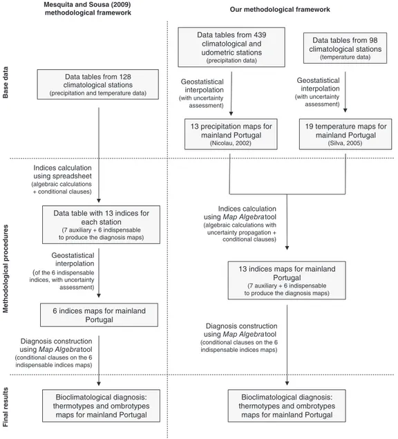
On the basis of RMWBCS, Mesquita and Sousa (2009) published maps of bioclimatological indices and a bioclimatological diagnosis for mainland Portugal using geostatistical techniques. The authors used air temperature and precipitation data from 128 climatological stations (corresponding to 96 Portuguese and 32 Spanish ones), referring to the 1961–1990 period, having rejected data series with less than 18 years of measurements. For each of the 128 data points, 13 bioclimatological indices were cal-culated. Six of them are indispensable to produce the final diagnosis maps, specifically: annual positive temperature (Tp), compensated thermicity index (Itc), annual ombroth-ermic index (Io), ombrothombroth-ermic index of the warmest bimonth of the summer quarter (Ios2), ombrothermic index of the summer quarter (Ios3) and ombrothermic index of the summer quarter plus the previous month (Ios4). The other seven are auxiliary indices necessary to obtain the former. The six indispensable indices were then interpolated (mapped) for mainland Portugal using four different mathematical techniques. Using cross validation (leave one out) the authors produced six evaluation mea-sures for each interpolation (see also Mesquita, 2005). The authors considered as best performing techniques: (i) kriging with external drift of a multiple linear regression for indices Itc, Io, Ios4 and Tp; and (ii) multiple linear regression followed by ordinary kriging of the residuals for Ios2 and Ios3. The six maps (with 1 × 1 km spatial resolution) obtained with the best techniques were used to construct the final diagnosis maps of thermotypes and ombrotypes, for the territory of Portuguese mainland. The first column of Table 1 presents a résumé on Mesquita and Sousa’s work.
Our aim was equally to produce a bioclimatological diagnosis for mainland Portugal according to RMWBCS, although using a different methodological framework and keeping track of the uncertainties associated with the pro-duced maps of bioclimatological indices.
2. Methodology
In this work, in spite of using the data of each climatologi-cal station to firstly climatologi-calculate the bioclimatologiclimatologi-cal indices and, subsequently, execute the geostatistical interpolation of the obtained indices (as e.g. in Mesquita and Sousa, 2009), we collected, as base data, geostatistical interpo-lations of precipitation and air temperature for mainland Portugal and, afterwards, calculated RMWBCS indices. The uncertainties associated with the base data were prop-agated using appropriated techniques. The indices maps were then used to obtain the bioclimatological diagnosis of mainland Portugal according to RMWBCS. The following subchapters present a detailed description of the method-ology used.
2.1. Base data
The base data employed in this work come from the spatial interpolations of the precipitation and air temperature of
mainland Portugal, achieved by means of geostatis-tical methodologies obtained by Nicolau (2002), for precipitation, and Silva (2005) for air temperature (see also Silva et al., 2007).
Nicolau (2002) aimed at discussing the performance of different mathematical techniques used for the spatial interpolation of point-associated information, in the con-struction of precipitation maps. As a result, for the territory of the Portuguese mainland, she carried out and produced a remarkable set of different analysis and precipitation maps, testing 10 different interpolation methods. The pre-cipitation series used were previously treated by, namely: pre-selection (rejecting precipitation series with less than 19 years of measurements); adjustment; and no-data fill-ing (among other tests and corrections). The result was a total of 439 series (corresponding to Portuguese clima-tological and udometric stations), used for the production of the final maps, covering the period between 1959/1960 and 1990/1991. A final set of 17 precipitation maps with 1 × 1 km spatial resolution was produced, using kriging interpolation and altitude as external drift. Five evaluat-ing measures were applied to each of the produced maps, obtained with cross validation (leave one out); Table 2 shows two of them used in this work: the mean absolute errors (MAE) and the root mean squared errors (RMSE). The MAE of an estimator T of a parameter 𝜃 (here 𝜃 is a precipitation or a temperature value in a location and T is the geostatistical interpolator) is defined as the expected value of |T − 𝜃|, and, similarly for the RMSE, as the square root of the expected value of (T − 𝜃)2. These error evalu-ation measures can thus be estimated averaging the abso-lute differences (or its squares) between the geostatistical estimates and the registered values, across all the used data points. The geostatistical estimate for each station’s location is obtained after removing that location from the data set.
As to the air temperature data, Silva (2005), after a pre-selection of the temperature series covering the 1961–1990 period (rejecting series presenting less then 20 years of measurements), used 98 sampled points (corre-sponding to 88 Portuguese and 10 Spanish climatological stations) to produce temperature maps, comparing eight different interpolation methods. To evaluate the methods performance, Silva opted for an external validation keep-ing 15% of the points apart for a subsequent evaluation and producing four evaluation measures (see Table 3 for MAE and RMSE). After selecting the best interpolation tech-nique (multiple linear regression using altitude and dis-tance from the coastline, with residuals kriging), 13 final maps were constructed employing the whole set of points, similarly with a 1 × 1 km spatial resolution. Subsequently to his work, Á. Silva (2006; pers. comm.) interpolated the mean minimum and maximum monthly air temperatures using the same methodology, as some of them are needed for the calculation of Itc; however MAE and RMSE are not available (consequently we could not calculate uncertainty propagation for Itc). Table 1 shows a comparative résumé of the three works referred in this article.
Table 1. Comparative résumé of the work of Mesquita and Sousa (2009), Nicolau (2002) and Silva (2005).
Mesquita and Sousa (2009) Nicolau (2002) Silva (2005)
No. of input data points (Portuguese + Spanish) 96 + 32 439 88 + 10
Data pre-treatments Pre-selection X X X Adjustment X No-data filling X Interpolation techniques Polynomial interpolation X Thiessen polygons X Triangulation X
Inverse distance weighting X X
Splines X X
Simple linear regression X X
Multiple linear regression X X
Ordinary kriging X X X
Kriging with external drift Xa Xa
Simple linear regression with residuals kriging X
Multiple linear regression with residuals kriging Xa Xa
Co-kriging X X
Neuronal networks X
Evaluation methodology
Cross validation (leave one out) X X
External validation (leave 15% out) X
Evaluation measures
Mean error X X X
Maximum error X
Mean absolute error X X X
Root mean squared error X X X
Percentage mean absolute error X X
Pearson correlation X X X
aSelected technique by the authors for the production of final maps.
Table 2. Evaluation measures for the estimated precipitation, obtained with cross validation; drawn from Nicolau (2002).
Symbols Precipitation MAE (mm) RMSE (mm)
P Annual (total) 101.42 150.80 P1 January mean 16.78 25.01 P2 February mean 16.00 23.18 P3 March mean 10.40 16.04 P4 April mean 8.19 12.16 P5 May mean 6.84 10.36 P6 June mean 4.28 6.33 P7 July mean 1.97 2.88 P8 August mean 1.88 2.95 P9 September mean 4.61 7.31 P10 October mean 10.97 15.91 P11 November mean 13.02 18.77 P12 December mean 16.40 23.99
2.2. Base data adjustments
Because the base data came from different sources, some previous adjustments were made in order to allow their concurrent use.
As to the air temperature, Silva (2005) treated 30 years of data, whereas, Nicolau precipitation data (2002) covers a period longer by 2 years, since she treated hydrological, and not civil year series. However, this difference is not expected to be relevant, because only mean values are concerned. Both authors used the same projection and
Table 3. Evaluation measures for the estimated air temperatures, obtained through external validation; drawn from Silva (2005).
Symbols Temperature MAE (∘C) RMSE (∘C)
T Annual mean 0.381 0.444 T1 January mean 0.520 0.602 T2 February mean 0.601 0.743 T3 March mean 0.414 0.522 T4 April mean 0.378 0.449 T5 May mean 0.299 0.370 T6 June mean 0.347 0.439 T7 July mean 0.520 0.657 T8 August mean 0.485 0.647 T9 September mean 0.519 0.624 T10 October mean 0.393 0.475 T11 November mean 0.536 0.646 T12 December mean 0.541 0.653
Tmin12 December mean minimum N/Av N/Av
Tmin1 January mean minimum N/Av N/Av
Tmin2 February mean minimum N/Av N/Av
Tmax12 December mean maximum N/Av N/Av
Tmax1 January mean maximum N/Av N/Av
Tmax2 February mean maximum N/Av N/Av
N/Av, not available.
georeferencing system, obsolete now: datum Lisbon; Hayford ellipsoid (or International 1924) and Mercator Transverse projection, with mainland Portugal parameters and coordinates origin in the Fictitious Point west of the S. Vicente Cape (Instituto Geográfico Português,
2009). Therefore, no projection adjustments were needed for the indices calculation. However, the bioclima-tological data here produced have been transformed to the updated coordinate system PT-TM06-ETRS89, using the Bursa-Wolf transformation parameters pro-vided by the IGP (Instituto Geográfico Português, 2009).
Even if the maps produced by Silva and Nicolau have the same 1 × 1 km spatial resolution and coordinate sys-tem, a 570 m displacement exists between the two grids of interpolated points (or pixels). Given that the original sur-faces resulting from the interpolations were not accessible, a possible solution would be interpolating the values from one of the grids to the locations of the other grid points, using GIS simple interpolation techniques (e.g. bilinear or cubic convolution). However, given the displacement and spatial resolution of the data, this procedure would result in a set of smoothed values, particularly in mountain-ous areas. Thus, the interpolation of new values between the original ones, while keeping the latter, was the chosen option. The Resample tool of ArcMap™9.2 SP5 (the used GIS software) was employed, selecting the cubic convo-lution technique and choosing a spatial resoconvo-lution which allowed the maintaining of the original values [in this case: 111.(1) m]. As a result, points were added to the original grids, thus achieving final grids with a spatial resolution of 111.(1) × 111.(1) m. Consequently, the initial displace-ment was reduced to approximately 60 m, that can be con-sidered negligible in view of the magnitude of other errors associated with the base data.
Silva and Nicolau did not use the same Portuguese bor-derline to cut out the final maps (estuaries and lagoons were treated differently by the authors: Silva (2005) excluded the air temperature data relative to these areas). Similarly, a number of locations next to the frontier lost cartographical representation (because the corresponding pixel centre fell out of the chosen mask). Given the unavail-ability of the original interpolated surfaces, as previously referred, these data absences were filled up with the near-est neighbour values, employing the Nibble tool from the same GIS software. For both reasons, the use and interpretation of values associated to the borderline, as well as to estuaries and lagoons, must be considered with caution.
2.3. Maps of bioclimatological indices
In order to obtain the maps of bioclimatological indices, the Map Algebra tool (from the used GIS software), which allows point-to-point operations between super-posed grids, was used to perform algebraic calculations with the collected base data, following the formulas pro-posed by RMWBCS (Rivas-Martínez et al., 2011).
Table 4 contains the list of the 13 maps of bioclimato-logical indices produced for mainland Portugal (needed to construct RMWBCS diagnosis maps). The abbreviations were kept as close as possible to those of Rivas-Martínez
et al.(2011). For the Map Algebra instructions please refer
to Monteiro-Henriques (2010).
Table 4. Bioclimatological indices computed for mainland Portugal.
Symbols
Tmax Mean temperature of the warmest month of the year
Tmin Mean temperature of the coldest month of the year
Tp Annual positive temperature (sum of the positive monthly mean temperatures, in Celsius degree ×10)
Pp Positive precipitation (sum of the monthly precipitation, relative to months with positive mean temperature)
M_maiusc Mean maximum temperature of the coldest month (M parameter, in the RMWBCS) M_minusc Mean minimum temperature of the coldest
month (m parameter, in the RMWBCS) Ic Simple continentality index, or annual thermal
amplitude
It Thermicity index
Itc Compensated thermicity index Io Annual ombrothermic index
Ios2 Ombrothermic index of the warmest bimonth of the summer quarter
Ios3 Ombrothermic index of the summer quarter Ios4 Ombrothermic index of the summer quarter plus
the previous month
2.4. Uncertainty propagation and significance tests Error and uncertainty propagation, especially when related to GIS operations and data processing, is a well-known and relatively studied problem (Heuvelink, 1998; Heuvelink and Burrough, 2002; Zhang and Goodchild, 2002). Nonetheless, its execution is complex, and implemen-tations capable of automatic and seamless propagation in current GIS are not yet known. Still, it is important to quantify uncertainty and assess how gravely can the output of models be affected by the use of input infor-mation that contains it (Bachmann and Allgöwer, 2002; Canters et al., 2002; Oksanen and Sarjakoski, 2005; Van Niel and Austin, 2007). Thus, uncertainty propagation for the maps of bioclimatological indices here pro-duced results pertinent for possible future analysis using this data.
In this subchapter we present the formulae used in the propagation of the uncertainty measures (MAE and RMSE) associated to the base data. The propagation of uncertainties is a consequence of the algebraic calculations carried out for the construction of the maps of bioclimato-logical indices, and is usually analytically deduced, or sim-ulated using the Monte Carlo method (Heuvelink, 1998). Coupled with geostatistical approaches, the Monte Carlo method allows the spatial analysis of uncertainties (see e.g. Temme et al., 2009; Hengl et al., 2010). In this work we focused on global measures of uncertainty (MAE and RMSE), which would allow the statistical comparison of our results to previous works. Our approach is particularly useful in the following common situation: the researcher has access to the variables maps and global error measures,
Table 5. Ombrotype and respective lower and upper horizons thresholds.
Ombrotypes Ombrotypes horizons Io
Ultrahyperarid Lower 0.0–0.1 Upper 0.1–0.2 Hyperarid Lower 0.2–0.3 Upper 0.3–0.4 Arid Lower 0.4–0.6 Upper 0.6–1.0 Semiarid Lower 1.0–1.4 Upper 1.4–2.0 Dry Lower 2.0–2.7 Upper 2.7–3.6 Subhumid Lower 3.6–4.6 Upper 4.6–6.0 Humid Lower 6.0–8.5 Upper 8.5–12.0 Hyperhumid Lower 12.0–17.0 Upper 17.0–24.0 Ultrahyperhumid Lower 24.0–33.9 Upper >33.9
but not to the original data (e.g. meteorological stations data), nor to maps depicting error variation in space.
For maps with the spatial representation of uncertainties associated with the variables maps used as base data in our work, please refer to the original works of Silva (2005) and Nicolau (2002).
As said before, the bioclimatological indices of RMW-BCS are of very simple calculation, and can be written linearly as x + k, k · x, x ± y or non-linearly as x/y, or com-binations of these four expressions, where x and y are climatological variables (Tables 2 and 3) or bioclimato-logical indices (Table 4) and k is a constant. We propa-gated the uncertainties in x and y, aiming to state the MAE and RMSE of the bioclimatological indices in terms of the known MAE and RMSE of x and y.
Assuming that the geostatistical interpolator is unbiased and that the errors of the estimated temperature and pre-cipitation are independent in each location, as well as between different locations, it is straightforward to show that:
MAEx±k= MAEx; RMSEx±k = RMSEx MAEkx= |k| MAEx; RMSEkx= |k| RMSEx
MAEx±y≤MAEx+ MAEy; RMSEx±y= √ RMSE2 x+ RMSE 2 y
Taylor expansion is frequently used to approximate errors coming from a non-linear expression (Heuvelink, 1998; Zhang, 2006). Consider ̂x an estimate of x, and
𝜀
x= x − ̂xthe error associated to that estimate. Using the first order expansion of x/y around ̂x∕̂y we have:
x y ≈ ̂x ̂y+ 1 ̂y ( x− ̂x)− ̂x ̂y2 ( y− ̂y) and 𝜀 x∕y≈ 1 ̂y𝜀x− ̂x ̂y2𝜀y
thus, the uncertainty measures may be estimated as MAE-T and RMSE-T:
MAE − Tx y ≈ 1 n n ∑ i=1 ( 1 ̂ yiMAEx+ | |̂xi|| ̂y2 i MAEy ) RMSE − Tx y ≈ √ √ √ √ 1 n n ∑ i=1 ( 1 ̂y2 i RMSE2 x+ ̂ x2i ̂ y4iRMSE 2 y )
where n is the number of sites for which x and y have been estimated.
As these expressions are only approximate, we also deemed the error propagation under the following pes-simistic perspective: | | |𝜀x∕y|||= | | | | | ̂x+ 𝜀 x ̂y+ 𝜀 y −̂x ̂y | | | | | ≤ | | | | | | | ̂ x+ ||𝜀x|| ̂ y− || |𝜀y||| −̂x ̂y | | | | | | |
This perspective is similar to combining the error signs in x and y in the most unfavourable way to produce the maximum propagated uncertainty for the values coming from ̂x∕̂y.
We considered replacing |𝜀x| and |𝜀y| by MAEx and MAEy, respectively: MAE∗ x y = 1 n n ∑ i=1 | | | | | ̂x i+ MAEx ̂y i− MAEy −̂xi ̂y i | | | | |
Similarly, we considered replacing |𝜀x| and |𝜀y| with RMSExand RMSEy, thus obtaining (recall that |𝜀|2= 𝜀2):
RMSE∗ x y = √ √ √ √ √ 1 n n ∑ i=1 ( ̂x i+ RMSEx ̂y i− RMSEy −̂xi ̂y i )2
For the case of Io, we found through a Monte Carlo study that MAEx y ≤MAE∗x y and RMSEx y ≤RMSE∗x y . We gener-ated 1000 samples with size n from the normal distribu-tion for the errors in temperature and in precipitadistribu-tion, and compared the ‘true’ (MAE and RMSE) and approximate (MAE* and RMSE*) uncertainty measures for Io. These unfavourable uncertainty measures (worst-case analysis) will be denoted by MAE-W and RMSE-W.
Some indices imply the use of conditional clauses, e.g. Ios2 is calculated from the mean temperatures and precip-itations of the warmest bimonth of the summer quarter. We neglected errors coming from the use of conditional clauses (e.g. the error in deciding which is the warmest bimonth of the summer quarter).
Assuming that 𝜀x/y are normally distributed with mean zero (as in the simulation study), we also checked for statistically significant differences between our results and those obtained by Mesquita and Sousa (2009) using an
F-test, where the alternative hypothesis was that RMSE2
were different. The p-values of the test were computed using the function pf () of the R statistical software, version 3.0.1 (R Core Team, 2013).
Indices calculation using Map Algebra tool (algebraic calculations with uncertainty propagation + conditional clauses) Indices calculation using spreadsheet (algebraic calculations + conditional clauses) Geostatistical interpolation (of the 6 indispensable indices, with uncertainty assessment) Geostatistical interpolation (with uncertainty assessment) Base data
Data tables from 439 climatological and udometric stations (precipitation data)
Data tables from 98 climatological stations
(temperature data)
Methodological procedures
Final results
Mesquita and Sousa (2009)
methodological framework Our methodological framework
Geostatistical interpolation (with uncertainty assessment)
13 precipitation maps for mainland Portugal
(Nicolau, 2002)
19 temperature maps for mainland Portugal
(Silva, 2005)
Data table with 13 indices for each station (7 auxiliary + 6 indispensable to produce the diagnosis maps)
6 indices maps for mainland Portugal Diagnosis construction using Map Algebra tool (conditional clauses on the 6 indispensable indices maps)
Bioclimatological diagnosis: thermotypes and ombrotypes
maps for mainland Portugal
13 indices maps for mainland Portugal (7 auxiliary + 6 indispensable to produce the diagnosis maps)
Diagnosis construction using Map Algebra tool (conditional clauses on the 6 indispensable indices maps)
Bioclimatological diagnosis: thermotypes and ombrotypes
maps for mainland Portugal Data tables from 128
climatological stations (precipitation and temperature data)
Figure 1. Methodological frameworks used in Mesquita and Sousa (2009) and in this work.
2.5. Bioclimatological diagnosis
Finally, we constructed the bioclimatological diagnosis for mainland Portugal, presenting two of the most important bioclimatological maps producible from RMWBCS: the thermotype and ombrotype maps.
A thermotype map is obtained with conditional clauses over three maps: macrobioclimates, Itc and Tp; thus an intermediate layer of macrobioclimates was constructed according to the RMWBCS, using conditional clauses of the ombrothermic indices (Io, Ios2, Ios3 and Ios4). In Portugal, only Mediterranean and temperate macrobiocli-mates are present. The ombrotype map is also obtained with conditional clauses over Io (corresponding to a sim-ple classification of Io in predefined intervals). Yet, we did minor adjustments to the subdivision of ombrotypes (the limits between each ombrotype upper and lower horizons), given that the ombrotypes limits suggested by RMWBCS have exponential adjustment (R2= 0.9961). The new sub-divisions (see Table 5) were computed after the logarithmic
transformation of the Io scale, thus avoiding the system-atic spatial under-representation of the upper horizons. The major divisions (between each ombrotype) were kept as in the RMWBCS.
The conditional clauses used were implemented using the referred Map Algebra tool of the mentioned GIS software, following the thresholds proposed by Rivas-Martínez et al. (2011).
Figure 1 shows the methodological frameworks followed by Mesquita and Sousa (2009) and in this work.
3. Results
3.1. Maps of bioclimatological indices
Figures 2 and 3 show the maps produced for each bioclima-tological index (It index is omitted as practically undistin-guishable from Itc at the presented scale). Each raster map has 111.(1) × 111.(1) m resolution and is projected accord-ing to the parameters of PT-TM06-ETRS89 coordinate
Figure 2. Bioclimatological indices maps produced for mainland Portugal (Tmax, Tmin, Tp, Pp, M_maiusc and M_minusc).
system (Instituto Geográfico Português, 2009), neverthe-less users of this information should recall that the used base data has 1 × 1 km resolution. This information can be downloaded both in coloured JPG and ESRI GRID formats from http://home.isa.utl.pt/∼tmh/.
3.2. Uncertainty propagation and significance tests As to the uncertainty propagation, Table 6 resumes all the calculated uncertainty measures and compares them with the results of Mesquita and Sousa (2009). MAE come from Mesquita (2005).
For the simulation study, 1000 samples of size
n= 7 251 544 were generated as normal variates with zero mean and standard deviation equal to 53.262 for Tp and 150.794 for Pp (the RMSE for Tp and Pp, respectively, in Table 6). The maximum (across the 1000 values) ‘true’
MAE for Io was 0.7256 while the minimum MAE-W was 0.8784. Concerning the RMSE, the maximum ‘true’ RMSE for Io was 0.9265, while the minimum RMSE-W was greater than 1.14.
As the produced RMSE-W proved (in the simulation test) to be higher than the real (unknown) RMSE, we ran the significance F-tests using the squared RMSE-W. Table 7 shows the results of those tests, comparing the squared RMSE propagated for the worst case with those obtained by Mesquita and Sousa (2009).
3.3. Bioclimatological diagnosis
Finally, Figure 4 presents the obtained thermotype and ombrotype maps for mainland Portugal according to the last version of RMWBCS (Rivas-Martínez et al., 2011).
Figure 3. Bioclimatological indices maps produced for mainland Portugal (Ic, Itc, Io, Ios2, Ios3 and Ios4).
These maps can also be downloaded from http://home.isa. utl.pt/∼tmh/.
4. Discussion
The produced maps of bioclimatological indices presented quite satisfactory MAE and RMSE. Comparing with the previous work of Mesquita and Sousa (2009), all the prop-agated uncertainties presented lower values, either using Taylor’s formula or the worst-case analysis. The method-ological framework we used implies a large number of geostatistical interpolations: 32 (corresponding to pre-cipitation and temperature variables). Note that Mesquita and Sousa’s (2009) needed only six to achieve the same
diagnosis maps. From these 32 interpolations we ought to additionally compute 13 indices maps (seven auxiliary and six indispensable to produce the final diagnosis). The fact that our approach uses a high number of geostatisti-cal interpolations and subsequent algebraic geostatisti-calculations could have lead to inflated final estimated errors, as error accumulates and amplifies in each consecutive calcula-tion. However, our approach permits the use of much more precipitation data as an input: Nicolau (2002) used not only data from climatological stations, but also data coming from the much more numerous udometric stations (where only data relative to precipitation is collected). The methodological framework followed by Mesquita and Sousa (2009) does not allow the use of data from udometric stations, as temperature data is lacking from
Table 6. MAE and RMSE estimated in this work and those estimated by Mesquita and Sousa (2009).
This work Mesquita and Sousa (2009)
Indices MAE RMSE MAE RMSE
Tmax 0.502 0.652 N/Ap N/Ap
Tmin 0.520 0.602 N/Ap N/Ap
Tp 45.720 53.262 57.938 74.378
Pp 101.419 150.794 N/Ap N/Ap
Ic 1.023 0.887 N/Ap N/Ap
Itc N/Av N/Av 12.218 15.601
MAE-T MAE-W RMSE-T RMSE-W
Io 0.075 0.773 0.089 1.139 1.005 1.751
Ios2 0.102 0.104 0.095 0.110 0.115 0.160
Ios3 0.153 0.157 0.122 0.141 0.176 0.255
Ios4 0.229 0.235 0.170 0.195 0.268 0.445
MAE-T, mean absolute errors propagated using Taylor’s formula; MAE-W, mean absolute errors propagated for the worst case; RMSE-T, root mean squared errors propagated using Taylor’s formula; RMSE-W, root mean squared errors propagated for the worst case. N/Av, not available, as the error of maximum and minimum temperatures where also not available. N/Ap: not applicable, as the index interpolation is not needed in the respective approach.
Table 7. F-tests checking for significant differences between RMSE2associated with bioclimatological indices.
Indices Fstatistic df1 df2 p-value
Tp 1.8251 127 13 0.2198
Io 2.3751 127 453 5.303e-11
Ios2 2.1538 127 453 7.328e-09
Ios3 3.2583 127 453 <2.2e-16
Ios4 5.2347 127 453 <2.2e-16
df1, degrees of freedom of RMSE2 from Mesquita and Sousa (2009);
df2, degrees of freedom of RMSE2propagated for the worst case, from
our work.
those sites and indices cannot be computed beforehand. Therefore, concerning precipitation data, the density of 1.2 input data points per 1000 km2 referred in Mesquita and Sousa (2009), is increased to 4.9 per 1000 km2in our approach, which certainly contributes to lower estimation errors.
Comparing to Mesquita and Sousa (2009), RMSE for Tp reduced 28% in our approach, although this difference did not result significant in the F-test. The magnitude of the differences in RMSE for the ombroth-ermic indices (Io, Ios2, Ios3 and Ios4) was higher (from 35% to 56%) and all resulted significantly different in the
F-test.
Taking into account that Nicolau (2002); Silva (2005) and Mesquita and Sousa (2009) used similar interpolation techniques, analyzing mostly the same period of time over the same region, and used similar criteria to pre-select data series, we conjecture that the magnitude of the differences between RMSE for the ombrothermic indices is proba-bly mostly related to the fact that Nicolau (2002) used a much greater number of input data points (accounting also for quality issues such as no-data filling and series adjustment), permitting to improve significantly the qual-ity of the precipitation estimations. In fact, Mesquita and Sousa (2009) referred that the obtained predictions for Io were too low in areas lacking climatological stations. Some residual areas of the centre east of Portugal presented very low and even negative values of Io, which produced
some unexpected areas of ultrahyperarid, hyperarid and arid ombrotypes (their absence from Portugal is widely accepted by experts). Such ombrotypes did not arise from our approach.
The produced bioclimatological maps and diagnosis were very satisfactory. A first assessment of their useful-ness and relationship with vegetation patterns at a local scale can be found in Monteiro-Henriques (2010); they were also revealed to be useful in other vegetation studies, at a regional scale, as can be attested in Pinto-Cruz et al. (2011).
Nevertheless, the belts found in the thermotype and ombrotype maps must be interpreted as climatologically similar zones, potentially containing characteristic flora and vegetation and not be assumed beforehand as the exact limits of flora and vegetation actually occurring in such areas. In the RMWBCS these thresholds are defined within a global perspective, consequently, they inevitably need to be adjusted to the local limits/ecotones (Gavilán, 2005). As RMWBCS proposes a finer subdivision of ombrotype and thermotype intervals (in upper and lower horizons), the adjustments up to the closest threshold can never be too large, and are frequently regarded as just negligible by the researcher, in view of the uncertainty normally associated to such limits. For this reason, the RMWBCS can be applied even at the local scale satisfying the researcher in his vegetation studies, allowing the potential comparison with other distant regions.
As our main conclusion, we showed that, at least in the Portuguese case, it is preferable to perform more geosta-tistical interpolations and calculation steps in the imple-mentation of RMWBCS (as it allows the use of udo-metric stations data), than performing less geostatistical interpolations (as it implies the discharge of data from udometric stations and use only data from climatological stations).
Finally it is worth mentioning that the uncertainty prop-agation procedure is rather time-consuming (the process was much longer than the construction of the correspon-dent indices maps).
Acknowledgments
We would like to thank: Rita Nicolau for the support given, particularly in the access to the base data used in this research; Felicity Anne Rowe for the English revi-sion; and three anonymous reviewers for their suggestions, which helped us to improve the manuscript. For this work, Monteiro-Henriques was financially supported mostly by a doctoral grant of Fundação para a Ciência e a Tecnologia (SFRH/BD/12356/2003) within Programa Operacional Ciência e Inovação 2010, III Quadro Comunitário de Apoio – Formação Avançada para a Ciência – Medida IV.3, and partially by a post-doctoral grant within Project SUSTAINSYS: Environmental Sustainable Agro-Forestry
Systems – NORTE-07-0124-FEDER-0000044
(ON.2-QREN-FEDER and PIDDAC-FCT-MEC). Cerdeira was partially supported by the Portuguese Foundation for Science and Technology through the Center of Mathemat-ics and Applications (CMA) within project UID/MAT/ 04106/2013. This work was also funded by the Fun-dação para a Ciência e a Tecnologia through the projects: UID/AGR/00239/2013 (Centro de Estudos Florestais) under FEDER/POCI; PTDC/AAC-AMB/113394/2009; and PTDC/AAC-AMB/111349/2009. We dedicate this work to Professor Salvador Rivas-Martínez.
References
del-Arco M, Salas M, Acebes JR, Marrero MD, Reyes-Betancort JA, Perez-de-Paz PL. 2002. Bioclimatology and climatophilous vege-tation of Gran Canaria (Canary Islands). Ann. Bot. Fennici. 39: 15–41.
del-Arco M, Perez-de-Paz PL, Acebes JR, Gonzalez-Mancebo JM, Reyes-Betancort JA, Bermejo JA, de-Armas S, Gonzalez-Gonzalez R. 2006. Bioclimatology and climatophilous vegetation of Tenerife (Canary Islands). Ann. Bot. Fennici. 43: 167–192.
Bachmann A, Allgöwer B. 2002. Uncertainty propagation in wildland fire behaviour modelling. Int. J. Geogr. Inf. Sci. 16: 115–127, doi: 10.1080/13658810110099080.
Cano E, Cano-Ortiz A, Del Río González S, Alatore Cobos J, Veloz A. 2012. Bioclimatic map of the Dominican Republic. Plant Sociol. 49: 81–90, doi: 10.7338/pls2012491/04.
Canters F, De Genst W, Dufourmont H. 2002. Assessing effects of input uncertainty in structural landscape classification. Int. J. Geogr. Inf. Sci.
16: 129–149, doi: 10.1080/13658810110099143.
Capelo J, Mesquita S, Costa JC, Ribeiro S, Arsénio P, Neto C, Monteiro-Henriques T, Aguiar C, Honrado J, Espírito-Santo D, Lousã MF. 2007. A methodological approach to potential vegetation mod-eling using GIS techniques and phytosociological expert-knowledge: application to mainland Portugal. Phytocoenologia 37: 399–415, doi: 10.1127/0340-269X/2007/0037-0399.
Costa JC, Neto C, Aguiar C, Capelo J, Espírito Santo MD, Honrado J, Pinto-Gomes C, Monteiro-Henriques T, Sequeira M, Lousã M, Lopes MC, Arsénio P, Jardim R, Alves P, Antunes JC, Pereira MD, Silva V, Ribeiro S, Gaspar N, Alves HN, Meireles C, Caraça R, Pereira EP, Martins M, Bingre P, Vila-Viçosa C, Mendes P, Canas RQ, Ferreira RP, Bellu A, Almeida JD, Caperta A, Vasconcelos T, Geraldes M, Almeida D, Gutierres F, Pinto JR, Mesquita S. 2012. Vascular plant communities in Portugal (Continental, the Azores and Madeira). Glob.
Geobot. 2: 1–180, doi: 10.5616/gg120001.
Font Tullot I. 2000. Climatología de España y Portugal. Ediciones Universidad de Salamanca: Salamanca, Spain.
Gavilán R. 2005. The use of climatic parameters and indices in vegetation distribution. A case study in the Spanish Sistema Central. Int. J.
Biometeorol. 50: 111–120, doi: 10.1007/s00484-005-0271-5.
Hengl T, Heuvelink GBM, van Loon EE. 2010. On the uncertainty of stream networks derived from elevation data: the error propagation approach. Hydrol. Earth Syst. Sci. 14: 1153–1165.
Heuvelink GBM. 1998. Error Propagation in Environmental Modelling
with GIS. Taylor & Francis: London, 127 pp.
Heuvelink GBM, Burrough PA. 2002. Developments in statisti-cal approaches to spatial uncertainty and its propagation. Int.
J. Geogr. Inf. Sci. 16: 111–113, doi: 10.1080/136588101100 99071.
Hijmans RJ, Cameron SE, Parra JL, Jones PG, Jarvis A. 2005. Very high resolution interpolated climate surfaces for global land areas. Int. J.
Climatol. 25: 1965–1978, doi: 10.1002/joc.1276.
Instituto Geográfico Português. 2009. Produtos do IGP –
Infor-mação Geodésica. http://www.igeo.pt/produtos/Geodesia/Inf_tecnica/ sistemas_referencia/sistemas_referencia.htm (accessed 12 February 2009).
Loidi J, Biurrun I, Campos JA, García-Mijangos I, Herrera M. 2007. A survey of heath vegetation of the Iberian Peninsula and Northern Morocco: a biogeographic and bioclimatic approach.
Phytocoenologia 37: 341–370, doi: 10.1127/0340-269X/2007/ 0037-0341.
Mesquita S. 2005. Modelação Bioclimática de Portugal Continental, Master thesis, Instituto Superior Técnico, Universidade Técnica de Lisboa, Lisbon.
Mesquita S, Sousa AJ. 2009. Bioclimatic mapping using geostatistical approaches: application to mainland Portugal. Int. J. Climatol. 29: 2156–2170, doi: 10.1002/joc.1837.
Monteiro-Henriques T. 2010. Landscape and Phytosociology of
the Paiva River’s Hydrographical Basin, PhD thesis, Instituto Superior de Agronomia, Universidade Técnica de Lisboa, Lisbon. http://home.isa.utl.pt/∼tmh/ (accessed 21 April 2015).
Monteiro-Henriques T, Espírito-Santo MD. 2011. Climate change and the outdoor regional living plant collections: an example from mainland Portugal. Biodivers. Conserv. 20: 335–343, doi: 10.1007/s10531-010-9864-3.
Nicolau R. 2002. Modelação e Mapeamento da Distribuição Espacial de
Precipitação – Uma Aplicação a Portugal Continental, PhD thesis, Faculdade de Ciências e Tecnologia, Universidade Nova de Lisboa, Lisbon.
Ninyerola M, Pons X, Roure JM. 2007a. Objective air temperature mapping for the Iberian Peninsula using spatial interpola-tion and GIS. Int. J. Climatol. 27: 1231–1242, doi: 10.1002/ joc.1462.
Ninyerola M, Pons X, Roure JM. 2007b. Monthly precipitation mapping of the Iberian Peninsula using spatial interpolation tools implemented in a Geographic Information System. Theor. Appl. Climatol. 89: 195–209, doi: 10.1007/s00704-006-0264-2.
Oksanen J, Sarjakoski T. 2005. Error propagation analysis of DEM-based drainage basin delineation. Int. J. Remote Sens. 26: 3085–3102, doi: 10.1080/01431160500057947.
Peel MC, Finlayson BL, McMahon TA. 2007. Updated world map of the Köppen-Geiger climate classification. Hydrol. Earth Syst. Sci. 11: 1633–1644.
Peinado M, Macias MA, Ocana-Peinado FM, Aguirre JL, Del-gadillo J. 2011. Bioclimates and vegetation along the Pacific basin of Northwestern Mexico. Plant Ecol. 212: 263–281, doi: 10.1007/s11258-010-9820-z.
Pinto-Cruz C, Barbosa AM, Molina JA, Espírito-Santo MD. 2011. Biotic and abiotic parameters that distinguish types of temporary ponds in a Portuguese Mediterranean ecosystem. Ecol. Indicators 11: 1658–1663, doi: 10.1016/j.ecolind.2011.04.012.
R Core Team. 2013. R: A Language and Environment for Statistical
Computing. R Foundation for Statistical Computing: Vienna. Rivas-Martínez S. 1996. Geobotánica y bioclimatologia – Discurso del
Acto de Investidura de Doctor Honoris Causa de la Universidad de Granada. Universidad de Granada: Granada, Spain.
Rivas-Martínez S, Rivas Sáenz S, Penas Á. 2011. Worldwide biocli-matic classification system. Glob. Geobot. 1: 1–634, doi: 10.5616/ gg110001.
Silva Á. 2005. Estimação da Temperatura Média do Ar em Portugal
Continental: Teste e Comparação de Métodos de Interpolação em Sistemas de Informação Geográfica, Master thesis, Instituto Superior
Técnico, Universidade Técnica de Lisboa, Lisbon.
Silva Á, Sousa AJ, Santos FE. 2007. Mean air temperature estimation in Mainland Portugal: test and comparison of spatial interpolation methods in GIS. In Proceedings from the Conference on Spatial
Interpolation in Climatology and Meteorology, Szalai S, Bihari Z, Szentimrey T, Lakatos M (eds). COST Office: Luxembourg, Germany, 262 pp.
Temme AJAM, Heuvelink GBM, Schoorl JM, Claessens L. 2009. Geostatistical simulation and error propagation in geomorphome-try. In Geomorphometry: Concepts, Software, Applications, Hengl T, Reuter HI (eds). Elsevier: Amsterdam, Netherlands and Oxford, UK, 121–140.
Thornthwaite CW. 1948. An approach toward a rational classification of climate. Geogr. Rev. 38: 55–94.
Van Niel KP, Austin MP. 2007. Predictive vegetation modeling for
conservation: impact of error propagation from digital elevation data. Ecol. Appl. 17: 266–80, doi: 10.1890/1051-0761(2007) 017[0266:PVMFCI]2.0.CO;2.
Zhang J. 2006. The calculating formulae, and experimental methods in error propagation analysis. IEEE Trans. Reliab. 55: 169–181, doi: 10.1109/TR.2006.874920.
Zhang J, Goodchild MF. 2002. Uncertainty in Geographical