Development and Testing of the Meta-Heuristic Hybrid DEEPSO

(1)

DEVELOPMENT AND TESTING OF THE

META-HEURISTIC HYBRID DEEPSO

FÁBIO MANUEL SOARES LOUREIRO

DISSERTAÇÃO DE MESTRADO APRESENTADA

À FACULDADE DE ENGENHARIA DA UNIVERSIDADE DO PORTO EM ENGENHARIA ELECTROTÉCNICA E DE COMPUTADORES

(2)

(3)

F

ACULDADE DE

E

NGENHARIA DA

U

NIVERSIDADE DO

P

ORTO

Development and testing of the

meta-heuristic hybrid DEEPSO

Fábio Manuel Soares Loureiro

Mestrado Integrado em Engenharia Electrotécnica e de Computadores Supervisor:: Pr. Dr. Vladimiro Henrique Barrosa Pinto de Miranda

Second Supervisor: Dr. Leonel de Magalhães Carvalho

(4)

(5)

Resumo

A maioria dos métodos de otimização com base estocástica, como é o caso dos Algoritmos Evolu-cionários, apresenta um conjunto de parâmetros que necessitam de ser ajustados: taxa de mutação, probabilidade de recombinação, fator de comunicação, entre outros.

No momento da apresentação dos algoritmos na comunidade científica, os desenvolvedores deste tipo de metodologias normalmente especificam um intervalo de valores para cada parâmetro que confere uma melhor performance ao algoritmo. Contudo a definição desse intervalo é baseado somente em algumas experiências realizadas. Uma incorreta parametrização condiciona todo o processo de otimização deste tipo de algoritmos, tornando a afinação de parâmetros num prob-lema especifico que requer alguma atenção no desenvolvimento de novos métodos de otimização evolucionários.

Desta maneira surge a necessidade da aplicação de um procedimento que encontre a con-figuração ótima dos parâmetros do algoritmo. Devido à sua dificuldade, a parametrização de algoritmos evolucionários assume-se como uma das mais importantes e promissoras áreas de in-vestigação ao nível da Computação Evolucionária.

Com vista à resolução do problema em questão, é proposta uma metodologia com base estatís-tica para afinação e comparação de Algoritmos Evolucionários. Métodos que utilizam o Planea-mento de Experiências introduzido por Ronald A. Fisher, como é o caso da Análise de Variância (ANOVA), apresentam um grande potencial neste campo . Por esta razão a ANOVA foi incluída na metodologia proposta.

Para aplicação da metodologia desenvolvida são utilizadas duas meta-heurísticas: EPSO (Evo-lutionary Particle Swarm Optimization), e o DEEPSO ( Differential Evo(Evo-lutionary Particle Swarm Optimization). Foram utilizadas três diferentes versões do DEEPSO, duas escolhidas que já tin-ham sido apresentadas, e outra que é proposta.

Ao longo deste documento, as duas meta-heurísticas utlizadas serão aplicadas a um conjunto de diferentes problemas de otimização. Para validação da metodologia proposta são aplicados a um conjunto de funções teste, sendo depois aplicados na otimização do trânsito de potências de duas redes de teste do IEEE de diferente dimensão e complexidade.

A análise dos resultados é focada às versões do DEEPSO testadas, uma vez que o EPSO apenas é utilizado para fins comparativos. Contudo foi igualmente submetido a todo processo que envolve a metodologia de afinamento e comparação. A metodologia foi aplicada com sucesso, sendo que o panorama geral dos resultados demonstra uma superioridade do DEEPSO Sg−rnd relativamente ao EPSO para problemas com maior dimensão e que apresentam mais dificuldade na sua otimização.

Palavras-chave: Optimização por Enxame de Particulas Evolucionário e Diferencial; Al-goritmos Evolucionários; Afinação de Parâmetros; Comparação de AlAl-goritmos ; Trânsito de Potências Óptimo .

(6)

(7)

Abstract

The majority of stochastic optimization methods, such as Evolutionary Algorithms (EA), have a range of adjustable parameters that need to be adjusted, like mutation rates, crossover probabilities and communication factors, among others.

At the moment of presentation of the algorithms to the scientific community, EA developers normally refer an optimal range of parameters values based on only a few experiments made. A poor algorithm parameterization hinders the discovery of good solutions. The parameter values needed for optimal algorithm performance are known to be problem specific that requires some attention on developing of new EA.

That is how that the needed for a parameter tuning procedure appears. Due to its difficulty, the issue of controlling values of various parameters of an evolutionary algorithm is one of the most important and promising areas of research in evolutionary computation.

To answer this problem, a statistical based methodology is proposed in this dissertation to precede a correct tuning and comparison of EA. The statistical methods, as Analysis of Variance (ANOVA), based on Design of experiments, which was firstly introduced by Ronald A. Fisher, seems to have a great potential in this field, and for this reason it was incorporated into this sys-tematic procedure purposed.

Two distinct heuristic methods are the basis to application of the developed methodology, the Evolutionary Particle Swarm Optimization, EPSO, and its hybrid called the Differential Particle Swarm Optimization Evolutionary, DEEPSO. Three versions of DEEPSO are tested, of those, two out of four have already been presented, that use the uniform recombination in sampling procedure, and another one that has been proposed here.

Throughout this document, DEEPSO and EPSO approaches will be applied to a set of different optimization problems. Firstly, in order to validate the proposed methodology, they have been applied in six well-known benchmark test functions and then, the case study, where EPSO and DEEPSO variants have been applied in an Optimal Power Flow (OPF) problem using two systems cases with different complexity and dimension (IEEE 57-bus system and IEEE 188 bus system).

The analyzed results are focused in the DEEPSO versions. EPSO is only used as compari-son with DEEPSO. However, it is also subjected to the whole process involving the tuning and comparison methodology. The proposed methodologies have been successful applied for both application cases (benchmark functions and OPF problem). The general overview of compari-son results shows that DEEPSO Sg−rnd performs better in more complex and larger dimension optimization problems, showing significant superiority to EPSO in these cases.

Keywords: Differential Evolutionary Particle Swarm Optimization; Evolutionary Algo-rithms; Parameter Tuning; Algorithm Comparison; Optimal Power Flow .

(8)

(9)

Acknowledgements

The quote that will be following presented has two different meanings for me. Firstly, I would like to thank the giants which worked with me at INESC TEC. For their unwavering support, motivation, and, above all, for their knowledge that helped me to complete this phase of my student life. However, it would be unfair to does not refer certain names : Pr. Vladimiro Miranda, particularly for the opportunity , Dr. Leonel Carvalho, for his availability and Carolina Marcelino, for a little of everything . I would also like to express my gratitude to Pr. Elizabeth Wanner, for hers knowledge in Statistical Analysis and hers patience to clear all my doubts.

However, I have been accompanied by giants since I was born, which have made me what I am today. Therefore, I would like to tanks to my father, my mother, my brother and my grandparents, for all their entire support and companionship. I would also like to thank all of my friends, which in one way or another also helped me growing up in all these years.

There are no amount of words that I could use to thank the person who supported me the most and gave me the strength and confidence to face this last challenge in my graduation, my love Liliana Lobo.

There is still a person that I would like to thank, my grandmother Maria, who despite no longer be here, was also a giant which marked my life for always and I know that today would be proud of me.

Fábio Loureiro

(10)

(11)

“If I have seen further, it is by standing on the shoulders of giants”

Isaac Newton

(12)

(13)

List of Figures

2.1 Gobal taxonomy of parameter setting in EA’s. . . 14

3.1 Sequence of optimization process of DEEPSO for Rosenbrock’s function using a population of 30 paritcles. For the black and white prints, the lighter squares represent the initial population, the medium light represents 15th generation and the darknest squares concern to final population . . . 24

3.2 A Black Box Process Model Schematic [1]. . . 25

3.3 Factorial experiment example of Table (3.3) and Table (3.4). . . 31

3.4 Boxplot graph description. . . 35

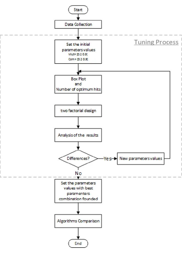
3.5 Proposed methodology for tuning and algorithm comparison. . . 38

4.1 Initial values tested for each parameter. . . 42

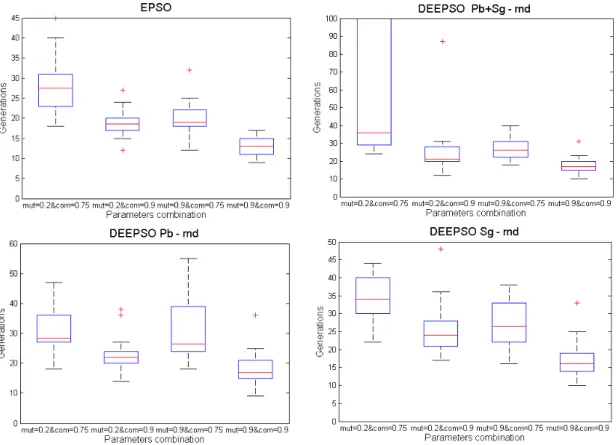
4.2 Bloxpot graphs of algorithm response for parameters values specifed in Figure4.1 . . . 43

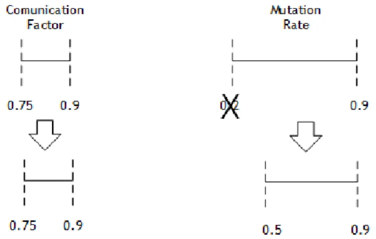
4.3 New values tested for each parameter in second iteration. . . 45

4.5 New values tested for each parameter in third iteration. . . 47

4.7 New values tested for each parameter in fourth iteration. . . 49

4.9 Number of hits on the optimum for 30 runs of each method tested. . . 52

4.10 Evolution of the average best fitness for 30 runs of EPSO and DEEPSO variants on Rastrigin’s Function. . . 53

4.11 Evolution of the average best fitness for 30 runs of EPSO and DEEPSO variants on Griewank’s Function. . . 53

4.12 Evolution of the average best fitness for 30 runs of EPSO and DEEPSO variants on Rosenbrock’s Function. . . 54

4.13 Evolution of the average best fitness for 30 runs of EPSO and DEEPSO variants on Damavandi’s Function. . . 54

4.14 Evolution of the average best fitness for 30 runs of EPSO and DEEPSO variants on Rotated Rastrigin’s Function. . . 55

4.15 Evolution of the average best fitness for 30 runs of EPSO and DEEPSO variants on Rotated Rosenbrock’s Function. . . 55

4.16 Boxplot graphs comparison for the four standart test functions used. . . 56

(16)

4.17 Boxplot graphs comparison for the Rotated versions of Rastrigin’s and

Rosen-brock’s functions. . . 57

4.18 Boxplot graph of Pb+Sg−rnd and Sg−rnd DEEPSO versions for Rosenbrock’s function. . . 58

5.1 Particle structure. . . 67

5.2 Evolution of the average best fitness for 30 runs of EPSO and DEEPSO variants on 57-bus system. . . 70

5.3 Evolution of the average best fitness for 30 runs of EPSO and DEEPSO variants on 118-bus system. . . 71

5.4 Boxplot graphs comparison of the best fitness value obtained for each system case. 71 5.5 Boxplot graphs comparison of the Pb+Sg−rnd and Sg−rnd DEEPSOs versions on 118-bus system . . . 72

5.6 Boxplot graphs comparison of the Computing time for each system case. . . 72

A.1 3-D map for 2-D Rastringin’s function. . . 79

A.2 3-D map for 2-D Griewank’s function. . . 79

A.3 3-D map for 2-D Damavandi’s function. . . 80

(17)

List of Tables

2.1 Main operators of EA schems . . . 7

3.1 Data arrangement for the one-way ANOVA. . . 27

3.2 one-way ANOVA table. . . 29

3.3 An example of a factorial experiment with two factors. . . 30

3.4 An example of a factorial experiment with two factors and with Interaction . . . . 30

3.5 Data arrangement for the two-factor factorial design. . . 32

3.6 Two-way ANOVA table . . . 34

4.1 Main features of the benchmark functions used. . . 40

4.2 Settings of external specified factors for each test function . . . 42

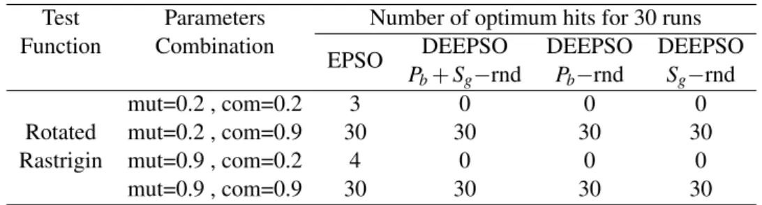
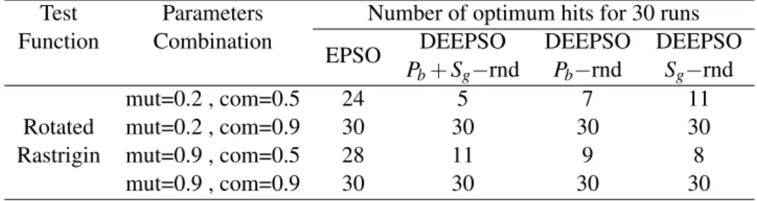
4.3 Number of optimum hits for 30 runs of each method for each parameters combi-nation. . . 44

4.4 Summary of two-way ANOVA results (Colums and Rows correspond to Commu-nication factor and Mutation rate, respectively). . . 44

4.5 Number of optimum hits for 30 runs of each method for each parameters combi-nation for second iteration. . . 46

4.6 Summary of two-way ANOVA results for second iteration (Colums and Rows correspond to Communication factor and Mutation rate, respectively). . . 46

4.7 Number of optimum hits for 30 runs of each method for each parameters combi-nation for third iteration. . . 48

4.8 Summary of two-way ANOVA results for third iteration (Colums and Rows cor-respond to Communication factor and Mutation rate, respectively). . . 48

4.9 Number of optimum hits for 30 runs of each method for each parameters combi-nation for third iteration. . . 50

4.10 Summary of two-way ANOVA results for fourth iteration (Colums and Rows cor-respond to Communication factor and Mutation rate, respectively). . . 50

4.11 Results of tuning procedure for all test functions(mut and com correspond to Com-munication factor and Mutation rate, respectively). . . 51

4.12 Variable used to distinguish the performance of algorithmos for each test function. 51 4.13 One-way ANOVA results for each test function. . . 57

4.14 One-way ANOVA results of DEEPSO versions comparison for each test function. 58 5.1 The different types of variables in OPF problem. . . 62

5.2 Summary of OPF methods [2,3,4]. . . 65

5.3 Caracteristics of each test case . . . 68

5.4 Settings of specified factors for each test case. . . 69

5.5 Results of tuning procedure for IEEE 57-bus system. . . 69

5.6 Results of tuning procedure for IEEE 118-bus system. . . 69

(18)

(19)

Abbreviations

AC Alternating Current DE Differential Evolution

DEEPSO Differential Evolutionary Particle Swarm Optimization EA Evolutionary Algorithm

ES Evolutionary Strategies EP Evolutionary Programming

EPSO Evolutionary Particle Swarm Optimization GA Genetic Algorithm

PSO Particle Swarm Optimization EC Evolutionary Computation OPF Optimal Power Flow

(20)

(21)

Chapter 1 Introduction

The first chapter of this Dissertation presents the main motivation for this work, a brief overview of the proposed methodology of tuning and comparison of Differential Evolutionary Particle Swarm Optimization (DEEPSO), and the major the objectives of this work and the main structure of this Dissertation. Lastly the organization of the thesis will be also explained.

Entire work behind this Dissertation was developed at INESC TEC under the supervision of Professor Vladimiro Miranda and Dr. Leonel Carvalho.

1.1 Motivation

Due to their general applicability, stochastic optimizers such as EA are popular among scientists and engineers facing difficult optimization problems. The most important components of EAs are thus recombination, mutation and selection. Recombination and mutation operators have param-eters in their implementation that need to be instantiated by a specific parameter value. On the other hand there are different approaches that can be used in the selection operator. Therefore, regardless of the type of EA, different algorithm’s configurations should be tested at the time of its development and presentation to the scientific community. The optimal configuration of the algo-rithm is specific for each optimization problem, and can not be defining an optimal combination of parameters based on a couple of examples of its application. Hence, a systematic procedure should be followed for EA tuning. Since EA have a probabilistic behavior, i.e. the results of an optimization performed by EA method vary from run to run and therefore, the performance evaluation must be performed using statistical based methods. In this way, a correct comparison of different optimization methods can be done, after finding their optimal configuration using a tuning procedure.

The DEEPSO method, as a new successful hybrid that was presented recently in scientific community, requires its application in other optimization problems in order to confirm its good convergence capabilities. However before performing the comparison with Evolutionary Particle Swarm Optimization (EPSO) in a set of different optimization problems, it is required to apply a tuning procedure to find the optimal configuration of both algorithms. These approaches have two

(22)

different parameters which play a crucial role in the optimization process: communication factor and mutation rate.

1.2 The purpose of this dissertation

The main objective of this dissertation is twofold: firstly, a new methodology is proposed that efficiently provides the tuning and comparison of EA; Then, the application of the methodology developed is made for three variants of DEEPSO and EPSO, evaluating its performance in set of different optimization problems. Both tuning and comparison procedures that incorporate the proposed methodology are statistical based, using designs of experiment: the two-way Analysis of variance (ANOVA) in the tuning process and one-way ANOVA for algorithms comparison. These statistical approaches only recently began to be successfully applied for this type of purposes, despite being a tool that has long been developed. In this procedures it is also analyzed other performance indicators such as the number of optimum hits in the optimum in a set of several runs and the evolution of average best fitness throughout the generations.

The development of this tool aims to perform a correct, scientific and fair comparison between the new approach so-called DEEPSO and EPSO. Furthermore there was a careful selection of the problems for the algorithms in testing in order to observe how they behave in different function landscapes and in the presence of constraints or different types of variables (continuous, discrete, binary).

In this way the proposed methodology was applied to the tuning and comparison of EPSO and DEEPSO in order to verify the superiority evidenced by DEEPSO at the moment of its presentation to the scientific community.

1.3 Structure of this Dissertation

Several works and papers were reviewed in order to understand the methodologies already pro-posed that aim EA tuning and comparison. Chapter2 not only features a summarized survey of most important existing tuning and comparison methods but it is also provided literature review concerning the topics on which DEEPSO is based: EA, Swarm intelligence, Differential Evolution (DE).

After reviewing the literature, in chapter3, the proposed methodology is presented, with all the tools used in its implementation being described in detail. Furthermore the entire formulation of DEEPSO is carefully analyzed and its also displayed two new versions of this algorithm.

Chapters4and5 refer the to application of the methodology developed to test the DEEPSO and EPSO in different optimization problems. Chapter4 features an experimental validation of the developed methodology, performing using a set of benchmark functions commonly used in the field of computational intelligence for evaluating algorithms performance. In section 4.3 it is described entire tuning procedure. Chapter5 presents the case study, with application of EPSO

(23)

1.3 Structure of this Dissertation 3

and DEEPSO versions on a typical power systems problem: Optimal Power Flow (OPF). Both tuning and comparison procedures are also applied to this problem.

Finally, the main conclusions are presented in Chapter6, featuring a few recommendations for future research in this field.

There are two appendix attached to this document: AppendixA, where it is presents an 3-D plot and a contour plot for each test function used in Chapter4; and AppendixB, which features the article containing an long abstract of developed work. This article will be submitted for a journal or conference for Power Systems.

(24)

(25)

Chapter 2 State of the Art

2.1 Evolutionary Algorithms – EA

Evolutionary algorithms form a class of meta-heuristic search methods that are often used for solving NP-hard optimization problems. In their general formulation it is easily perceptible sev-eral concepts inspired by behaviors observed in nature. For example, one of them is the natural selection process. In this process stronger individuals are the better prepared and adapted from all set of individuals, thus dominate weak individuals and thrive. Those individuals have some characteristic that distinguishes them from other members. Through inheritance this set of char-acteristics will have a very high chance of being gifted to their descendants and it will present themselves in the population for next generations.

Therefore Evolutionary Algorithms are inspired by Darwinist theories in an attempt to adopt biological evolution mechanisms [5]. From this theory of Darwinian evolution, the Evolutionary Programming (EP), as Evolution Strategies (ES) and Genetic Algorithms (GA) appeared in the early 60s [6] .

The application of genetic operators allows spawning of a new slightly different set of indi-viduals from an initial population that was randomly generated. Like each member of the initial population, these new individuals are possible successful candidates. However, they are generally a better fit than their parents. Mutation and recombination operators ensures the maintenance of individual diversity and pushes the population toward the optimum combination, while the selec-tion operator is responsible for the evoluselec-tionary characteristic of these algorithms and it is what defines who will be forming the next generation of the iterative process.

(26)

Below, we move on to a summary description of the each operator on which Evolutionary Computation is based and their general procedure:

procedure EA

Initialize a random population P of µ particles repeat

Reproduction (introduce stochastic pertubations in the new population)-generate λ offspring...

...by mutation ...by recombination

Evaluation - calculate the fitness of the individuals

Selection - of µ survivors for the next generations, based on the fitness value

until the convergence criteria is satisfied (based on fitness, on mumber of generations, etc) end procedure

These algorithms have the goal of searching the optimal solution as their main objective, in-dependently of the variables nature. It all begins with the formation of a population, which will be the set of possible solutions for a given problem. Each individual of this population is evaluated by a function that we aim to optimize. From this evaluation process, a set of “best” individuals is selected for reproduction, forming the new generation. Then these new individuals undergo a new evaluation process to eliminate those with worse performance. Thus a subsequent generation is formed [5]. After this process, the evaluation and selection procedures are iteratively applied to generate the next generations. So, the “general population” will be enriched with individuals of increasingly better fitness. When a certain stopping criterion is satisfied, the supreme individual, from the final population, is proposed as the solution of the optimization problem.

The two different approaches of the EA models can be distinguished mainly through the way that the problem variables are encoded: the phenotype and genotype methods. When the solutions of the given problem are directly represented by its variables, it is a phenotype method. In turn, genotype methods are based on genetic representation by using binary chromosomes as a coded sequence. Both EP and ES algorithms are examples of the use of the phenotype representation without passing through any intermediate algorithm for coding/decoding processes. In contrast, canonical GA trusts in the power of a discrete genetic representation of each individual to generate new individuals with better chance of survival. This distinction relating to a variable representation is not always clear. A change of the decimal representation of a numeric variable to a binary representation does not necessarily transform an ES in a GA approach and the criterion of choice should be based on the simplicity and convenience of using one instead of the other. In addition, the type of selection and recombination procedure and the size of the population (parent/offspring) are points where there may be differences between EA variants [5] .

EA has been hybridized with knowledge-based systems, Artificial Neural Networks and Fuzzy systems for several applications in the field of Power Systems, but It also have a big potential for

(27)

2.2 Evolutionary Programming and Evolution Strategies vs Genetic Algorithms 7

applications in many other areas. In general, the characteristic problems in the area of power sys-tems represent nightmares for researchers and developers: integer variables, non-convex functions, non-differentiable functions, domains not connected, badly behaved functions, multiple local op-tima, multiple objectives, and presence of fuzzy data. This kind of problems can be solved by EA approaches with very successful results [7]. However, using EA for large-scale problems generally takes too much time, which can be a serious drawback in some problems. The way to get around this problem lies in the organization and use of computational clustering of machines connected on the same network. In this way, the increase of speed is almost proportional to the number of machines connected on this network without the need of any special processor architecture or pro-gramming language. Therefore, changing EA though the introduction of self-adapting parameters can be a good way to improve the efficiency of a problem, providing better chances to find the global optima in very complex problems.

2.2 Evolutionary Programming and Evolution Strategies vs Genetic

Algorithms

All EA variants use the same principles of the evolutionary computation, but are applied with different strategies. Besides the differences in the representation of Individuals, the distinction between ES e EP can also be done through the type of selection procedure applied, by usage (or not) of recombination or/and mutation operator [8].

Table 2.1: Main operators of EA schems

Strategy Mutation Recombination Tournament selection

ES yes yes Elitism

EP yes no Stochastic

GA yes yes Stochastic (spinning roulette)

In GA, the mutation operator (random negation of a bit position) is normally used with a lower rate compared to the crossover operator, which makes the recombination/crossover of the solutions the primary source of variation in the population (mutation is usually regarded as a background operator or is not employed). The GA is usually characterized by fitness-proportionate selection (stochastic selection method where the selection probability of an individual is proportional to its fitness). In order to be better tailored for the optimization in real-value search spaces, GA started adopting chromosomes with real variables instead of bit sequences. So, Real-coded GA appeared and, thereby, started to adopt similar representations used by ES and EP [8].

In the original/primitive EP the use of crossover technique has not been observed. However, presently, there is not much point in this question because there have been some EP variants using the crossover operator [5]. Despite being developed independently from each other, some researchers argue that EP is the offspring of a kind of a mix between GA e ES, and often consider it as a special case of ES. Unlike GA, ES and EP start to give more importance to the mutation operator, as opposed to the recombination/crossover operator. Traditionally, ES adopts elitism

(28)

(the forced selection of the best individuals) for selection procedure, while EP typically uses a stochastic tournament where it randomly chooses the individuals to form the next generation.

Ultimately GA and EP/ES are two branches of the EA family and therefore they have common characteristics, which are based on a selection process for a population with evolutionary character. Initially, in its canonical form, these two branches presented themselves very distinctively but nowadays it does not make sense to talk about their differences, even more when self-adaptive mutation schemes are introduced in their formulations. With the advent of Real-coded GA, neither in the field of variables representation there are differences because like EP/ES, this modern GA shows the advantage in the use of natural variables. Working with this representation of variable problems it is easier to visualize the search space created by genetic operators and eventually modify them to enhance the performance of the algorithm. In this way it becomes easier to try variations on the operators for including the improvements in the desired exploration of possible solutions and the search for promising regions (valleys which may be indicators of a possible/local optimal solutions). Furthermore, opting for this type of representation makes it rather easier to respect the restrictions that an optimization problem may have. The major theme of discussion in this field should be the definition of the model type and which algorithm to adopt when faced with a concrete optimization problem.

2.3 Swarm intelligence

2.3.1 Particle Swarm optimization - PSO

Particle swarm optimization (PSO) is a population based stochastic optimization technique devel-oped by Russell Eberhart and James Kennedy in 1995 inspired by the ability of flocks of birds, schools of fish, and herds of animals to adapt to their environment, find rich sources of food, and avoid predators [9]. For example, Flocks of birds fly in V-shaped formations to reduce drag and save energy on long migrations. It was from this type of behavior that appeared the main basis of this algorithm: information sharing and collaboration between individuals (sets of solutions that evolve in the space of alternatives, identified as particles) through simulation of social behavior [6].

PSO shares many similarities with evolutionary computation techniques such as GA. The sys-tem is initialized with a population of random solutions and searches for optima by updating the generations. However, unlike EA, instead of using traditional genetic operators, each particle (in-dividually) adjusts its direction of movement according to the movement that it had previously, its own movement experience (memory) and its companion’s movement experience (cooperation).

Based on the movement rule, each particle is assigned a position vector Xi , which represents a possible vector as basis for next iteration, a velocity vector Vi , responsible for switching the position of the particle, and a second position vector bi to save the position which is associated to its best fitness solution that it has achieved so far. Each particle also has a third position vector bg, where the position of the best solution ever found by the entire population is saved. The PSO

(29)

2.3 Swarm intelligence 9

concept consists of, at each time step, changing the velocity of each particle in the search space toward its best position and toward the swarms best position. The velocity term from movement equation depends on three main factors so-called inertia, memory and cooperation. One of the possible formulations of the velocity of each particle is given as follows:

Xinew=Xi+Vinew (2.1)

Vinew=Dec(t)wi0Vi+Rnd1wi1(bi− Xi) +Rnd2wi2(bg− Xi) (2.2)

Where i is the generation number and wik are diagonal matrixes representing the weights of

each term. These weights are affected by a random number Rndx, drawn from the [0,1] interval,

which causes a disturbance in the trajectory of each particle shown to be beneficial for space exploration and the discovery of the optimal solution. The first term of the equation, responsible for velocity updates, refers to the inertia of the particle and reflects the direction of the current motion. Linked to this term exists a function which decreases the importance of inertia term during the course of the algorithm. The second term represents the particles own memory, where the particle keeps the best position in its past life (particular best position). In the third term is represented the swarm influence. Similarly to the memory term, it is responsible for making the particle movement being attracted to the best point found by the entire population/swarm (global best position).

In the beginning of the process, weights associated to the memory and cooperation terms need to be initialized and an adequate tuning of these parameters is not always achieved. Due to this sensitivity shown by PSO, a fine tuning of the weights is particularly important for convergence to be achieved [10]. In the first experiments, PSO proved to be a successful and fast method to converge to optimum regions, nonetheless it has weak local search ability. The particle velocity was still excessive when it was close to the optimum, overshooting and making swarm convergence difficult to attain. This problem was solved by means of particle velocity control. One example of this control is the introduction of a decreasing function Dec(t) linked to the inertia term as it is showed in PSO formulation. A different formulation for commutation of particles velocity can be also applied using a constriction factor, which affects the weights in each iteration in order to obtain a convergence control[5].

Another important issue concerns the timing of the updates of the particles best positions and the global optimal position found by the entire swarm. In this way it is necessary to determine if each particle is attracted by the latest global optimum or if the update of the current optimum is done only at the end of the current update cycle of all particles (after each iteration) [5].

2.3.2 Evolutionary Particle Swarm Optimization – EPSO

As opposed to EA, no selection operator appears in PSO formulation and all initial particles of the swarm are kept until the end, and, consequently, in this approach there is no competition between

(30)

particles [11,5]. However it is possible to interpret PSO as an ES. There is several similar char-acteristics: a fitness function (for each particles position in the search space corresponds a fitness value), a set of individuals (particles) which form a population (swarm), recombination (parti-cles exchanges information), mutation (weights of memory and cooperation terms are randomly set at each iteration) and reproduction (based on the movement rule applied to each particle)[6]. In practical terms, the high dependence of the external control schemes is considered to be the only drawback of PSO, being necessary to define external parameters recurring to a trial and error methodology.

In this context emerged Evolutionary Particle Swarm Optimization which puts together con-cepts from both EA and PSO. Self-adaptation concon-cepts are firstly introduced in PSO formulation by Miranda and Fonseca [10]. This hybridization of PSO with EA allowed a huge improvement in exploring the search space around the optimum value. Like the PSO algorithm, EPSO uses a swarm of particles evolving in the search space through a movement rule, however, these particles will also be subject to selection under the evolutionary paradigm [10,12,13]. Once the efficiency of the reproduction process is constrained by the influence of weight values in the movement equa-tion, a self-adapting propriety needs to be added in the strategic parameters. In this way, the initial value specified for weights loses its relevance in the EPSO mechanism, since the selection proce-dure also operates at the level of the weight values, selecting those which give the best efficiency in the algorithms convergence to the optimal. Despite using swarm intelligence, EPSO follows an evolutionary scheme as any other EA and therefore, it has the following operators implicit in its implementation:

procedure EPSO

Initialize a random population P of µ particles repeat

Replication - each particle is replicated r − 1 times

Mutation - each particle has its strategic parameters mutated

Reproduction - each mutated particle generates an offspring according to the movement equation

Selection - by stochastic tournament or elitism, the best particle of each offpring group (with r offpring) of each individual belonging to the previous generation is selected to form a new generation

until the convergence criteria is satisfied (based on fitness, on mumber of generations, etc) end procedure

An important point to be noted is the selection procedure. The particle which corresponds to the global best is treated in a different way than the rest of the swarm: it is not eliminated unless one of its descendants finds a better point and replaces it [14]. Therefore, selection only happens after acting upon the generation that is already better than its parent. Then, using a stochastic tournament (or elitism), the best particle among the offspring of each particle from the previous

(31)

2.3 Swarm intelligence 11

generation, is selected with probability (1 − Luck), where the luck parameter is set by a very low value.

For an EPSO algorithm, the movement equation that is going to be applied is obtained by the following formulation (the symbol ∗ in the following formulations indicates that these parameters will undergo evolution through mutation):

Xinew=Xi+Vinew (2.3)

Vinew=w∗i0Vi+w∗i1(bi− Xi) +w∗i2(b∗g− Xi) (2.4)

A new particle Xnew

i is obtained much like the way which is observed in the PSO approach.

However, the mutation of the weight values is ruled by a multiplicative Log-normal distribution obtained from Gaussian distribution where the mean equals 0 and the variance equals to 1:

w∗

ik=wik[LogN(0,1)]τ (2.5)

Where τ is the mutation rate which must be fixed externally to control of the mutations ampli-tude on weight values.

Alternatively a multiplicative or an additive mutation procedure can be followed:

w∗

ik=wik(1 + σ × N(0,1)) (2.6)

w∗

ik=wik+ σ× N(0,1) (2.7)

Where σ has an equivalent function to that of the mutation rate τ but in these mutation schemes σ must be small enough to be possible to control the weights in order to avoid that its values becomes negative.In the case of being used an additive mutation procedure, as presented in (2.7), the mutation value is insensitive to the value of wik. For this reason, multiplicative mutation

schemes, such as in (2.6), are more common in Evolution Strategies [5].

In addition, another important difference between EPSO and PSO can be observed, more precisely, on how both algorithms treat the global best value in the cooperation term. In the EPSO approach, this value also undergoes mutation . Then as it is shown in the expression (2.8), the global best particle is affected by an additive mutation scheme, which introduces a distortion in the attraction effect of the global best.

b∗

g=bg+w∗i3N(0,1) (2.8)

Where bg is the global best and w∗i3 is a new weight, which has also to been mutated. This

weight is responsible for controlling the amplitude of this introduced disorder.

With this new targets of the mutation procedure, in EPSO methodology is being avoided that particle’s convergence towards to the same region of the search space. Also in this context, a

(32)

stochastic scheme for the communication topology was presented [15,13]. This new approach oscillates between purely cognitive model and the star model, where every particle is aware of the global optimum. Therefore, the improvement in the algorithm’s behavior is reached by using a communication factor P, which is a diagonal matrix linked to cooperation term in movement equation. Since it contains binary variables of value 1 with probability p, there is a probability (1 − p) in which a certain dimension of a particle that will not receive the information available on the best location found by the swarm [15]. This parameter p is a probability value defined in [0,1] and it leads to slower/faster propagation of information between particles. Consequently, by including this constrain in free flow of information it allows a better overall local search for each particle and avoids premature convergence.

Vnew

i =w∗i0Vi+w∗i1(bi− Xi) +P[w∗i2(b∗g− Xi)] (2.9)

So an adequate tuning of the communication factor will increase the convergence capabilities of EPSO as was proven in [15], where experimental results have suggested that a lower commu-nication probability leads, in some cases, to better results than a classical deterministic star model (with p = 1). However, this cannot be taken as a guaranteed fact, since the behavior of EPSO may show a different response when changing the probability of communication.

2.4 Differential Evolution – DE

Differential evolution follows the general procedure of an EA. It was firstly introduced in [16] as an efficient Heuristic for global optimization over continuous spaces. Differential evolution follows the general procedure of an evolutionary algorithm. Using an uniform distribution, the initial population of NP targets vectors −→Xi,Gis randomly generated for each generation G:

− →_X

i,G= [x1,i,G,x2,i,G,x3,i,G, ...,xD,i,G] , with i = 1,2,...,NP (2.10)

Each vector is a candidate solution to a D dimensional optimization problem that is being treated. After initialization of each , DE enters in the evolutionary procedure like the one that is illustrated below, using three operators: mutation, crossover and selection [17].

procedure DE repeat

Mutation - generate a donor vector −→Vi,G= [v1,i,G, ...,vD,i,G]corresponding to the ith

target vector −→Xi,G, using the differential mutation scheme

Crossover - generate a trial vector −→Ui,Gfor the ith target vector −→Xi,G trough binomial

(or binomial/uniform) crossover

Selection - after evaluate the target vector −→Xi,G and the trial vector −→Ui,G, both are

compared in order to define each one will form the population of the next generation until the convergence criteria is satisfied

(33)

2.4 Differential Evolution – DE 13

The mutation step can be applied by following a high number of different procedures. The five main formulations or also called learning strategies most used in literature are:

DE/rand/1 : −→Vi,G= −→Xri 1,G+F(− →_X ri 2,G− − →_X ri 3,G) (2.11)

DE/best/1 : −→Vi,G= −→Xbest,G+F(−→Xri 1,G−

− →_X

ri

2,G) (2.12)

DE/current to best/1 : −→Vi,G= −→Xi,G+F(−→Xbest,G−−→Xi,G) +F(−→Xri 1,G−

− →_X

ri

2,G) (2.13)

DE/best/2 : −→Vi,G= −→Xbest,G+F(−→Xri 1,G− − →_X ri 2,G) +F(− →_X ri 3,G− − →_X ri 4,G) (2.14) DE/rand/2 : −→Vi,G= −→Xri 1,G+F(− →_X ri 2,G− − →_X ri 3,G) +F(− →_X ri 4,G− − →_X ri 5,G) (2.15) Where indices ri

1,r2i,r3i,ri4 and ri5 are random and mutually different integers sampled from

[1,NP] and F is a scale factor ,which needs to be externally specified. Another parameter that must be specified is the crossover rate Cr, which responsible for recombination procedure control.

Actually the differences between the applied mutation schemes are in the selection of the base vector to be perturbed and in the number of difference vectors, which are considered for pertur-bation of the selected base vector. The type of crossover can also identify one DE scheme from another [16].

Neglecting recombination, DE then proceeds with a parent selection (selecting the next gen-eration from both the parent and offspring populations) of a special type – each parent competes only with its offspring [18].

By also using scaled difference vectors, PSO algorithm models the stochastic attraction toward the personal and global best positions in the movement equation for the velocity update. The DE has a similar behavior when picks up two random individuals (the equivalent of a particle in PSO approach) from the population. For exemple, the DE/current to best/1 scheme presented in expression (2.13) may be rewritten using the movement equation as in (2.1) and (2.2):

Xinew=Xi,G+Vinew (2.16)

Vinew=F(Xbest,G− Xi,G) +F(Xri

1,G− Xri2,G) (2.17)

In [19], Suganthan and Qin have proposed a hybrid DE algorithm that in its implementation had a self-adaptive strategy. For this Self-adaptive Differential Evolution (saDE) approach, it was not necessary that the value of the control parameters (F, Cr and NP) was specified. The saDE

also becomes independent from the learning strategy applied, since this algorithm adapts perfectly its mutation scheme for the specific problem. Zang and Xie [20] proposed another popular hybrid

(34)

algorithm called DEPSO, in which the original PSO algorithm and the DE operator alternate at the odd and even iterations.

2.5 Parameter tuning for EA

Parameterized EA has been a standard part of the Evolutionary Computation community from its inception. The widespread use and applicability of these approaches is due in part to the ability to adapt an EA to a particular problem-solving context by tuning its parameters. However, tuning EA parameters can itself be a challenging task since its parameters interact in highly non-linear ways on EA performance. In addition there is one aspect that normally is not taken to account by researchers when they use a tuning method: different algorithmic configurations are optimal at different search-stages of the optimization process. The optimization process implies a that it runs on a dynamic way from a more diffuse global search until a more focused local optimization process is achieved. To begin, it requires parametric values suited for the exploration of the fitness landscape and then it requires additional parameter values which help with the convergence of the algorithm, on a further stage.

In practice, parameter values are mostly selected by conventions (for example: mutation rate should be low in order to not introduce too much distortion in the optimization process ) or by the researchers experience when they present their meta-heuristics in the scientific community. In the vast majority of cases, they present their algorithm showing its best parameters based on few trials. An EA with good parameter values can be orders of magnitude better than one with poorly chosen parameter values [21].

Figure 2.1: Gobal taxonomy of parameter setting in EA’s.

Following the classification introduced in [22], which is exhibited in Figure (2.1), the methods for parameter setting in EA fall into one of two main categories: parameter tuning and parameter control. The criteria used for its differentiation is the timing of the tuning procedure. In the first category find the optimal parameter configuration prior to the optimization process. On the other hand, parameter control refers to starting the optimization process with a suboptimal parameter configuration and then optimize the parameters values during the search process.

(35)

2.5 Parameter tuning for EA 15

The methods used for parameter control can be sub-categorized by the way they change the parameter value during the execution of the algorithm. In the case of the deterministic approaches the modification of the strategy parameter occurs following a fixed, pre-specified way without using feedback from the search. In contrast, for adaptive and self-adaptive methods, the direction and/or magnitude of the change to parameter value results of feedback from search procedure. The big difference between them is the manner that is used to updating parameter values. The adaptive control uses an external scheme to update the value, while adaptive methods result from the use of the selection operator [22].

2.5.1 Measuring search effort

Obviously, good tuning algorithms try to find good parameter values with the least possible effort. This measure can be given using the following expression A × B ×C , where A is the number of distinct parameters to be tested by the tuner; B refers to the number of runs and C is the number of function evaluations performed in one run of the EA. The total number of algorithm runs used by the tuners is given by the product A ×B. An insightful survey and classification of tuning methods is present in [21,23], which summarize existing methods in four categories: tuners that allocate the search efforts by the minimization of A, B and C, respectively.

2.5.2 Survey of tuning methods

There are a several number of algorithmic approaches to solving the parameter tuning problem, by generating parameter vectors (which are solutions to parameter tuning problems) and testing them to establish their utility (performance criteria). This type of approach can be made in an iterative way, creating new vectors iteratively during execution, or in a non-iterative way, using a fixed set of vectors. Some of the most promising methods used for this purpose are presented hereunder.

2.5.2.1 Design of experiments

Many experiments, like tuning EAs, involve the study of the effects of two or more factors/parameters and a correct approach to dealing with this type of problems is to conduct a factorial experiment. This is an experimental strategy in which factors are varied together, instead of one at a time. The factorial experiment design concept is extremely important, and it can be easily applied for tuning procedures in EA. Another approach, more accurate than factorial experiments is Response Surface Methodology. This is an empirical model of the process and to obtain a more precise esti-mate an optimum solution of certain problems. This technique is usually applied after the factorial experiment is also applied. Both approaches are collections of mathematical and statistical tech-niques that are useful for the modeling and analyzing of problems in which a response of interest is influenced by several variables and the objective is optimize this response [24].

These statistical techniques are very efficient and rigorous. They allow the effects of each pa-rameter tested to be estimated at several levels. Furthermore, these methods can be useful to avoid

(36)

misleading conclusions when interactions of parameter effects may be present. The major draw-back in applying these methods in type of optimization problems like tuning EA is that requires a several runs of the algorithm for each combination to be tested. Generally these kinds of tools are used in a step in more complex procedures.

2.5.2.2 Meta evolutionary algorithms

Since the tuning procedure is a kind of optimization problem, EAs can be successfully applied for finding a good set of parameter values. This type of EA that are used for optimizing the parameters is called a meta-EA and any kind of EA (GA, ES, EP, DE, PSO, . . . ) can be used for this purpose. To modeling this problem, the individuals used in the meta-EA are the parameter vectors, which contain parameter values to be tested. Each individual (parameter vector) has a utility value, based on information regarding fitness. Using this utility information, the meta-EA can use the selection, recombination and mutation operator as it usually does. However, this method implies a large computational cost (large number of hours for this procedure tuning be completed) [25].

Another algorithm can be applied to find the optimal values of each parameter by using con-cepts like probability distributions and entropy for tuning process. This enhanced method denom-inates as the Relevance Estimation and Value Calibration (REVAC) and it can also give infor-mation about the costs and benefits of tuning each parameter. In essence, REVAC is a specific type of meta-EA where the population approximates the probability density function of the most promising areas of the utility landscape [26].

2.5.2.3 Sampling methods

This type of tuners appreciate the use of a small number of parameter vectors, which means that the search effort applied in the tuning procedure is reduced by cutting the number of the parameters tested. In this way its efforts are axed towards to a full factorial design. Most of non-iterative sampling methods are mainly used as an initialization step in more complex models.

The Latin-Square (used to construct row-column designs and also for eliminate nuisance sources of variability) [27] and Taguchi methods (by using orthogonal arrays and testing pairs combinations to reduce the variation in a process through robust design of experiments) [28] are the two most often used. Both methodologies are often incorporated in multi-stage and iterative sampling methods.

These multi-stage approaches delimit the drawing area of new points in each iteration. For instance, in [29] Adenso-Diaz et al. introduced CALIBRA for the first time, which consists of the combination of Taguchi’s fractional factorial experimental designs coupled with a local search procedure. This method only can be used in the tuning of optimizing EA performance and not for robustness, since it needs a quality measure to define a promising area. Furthermore, the number of parameters that it is capable of handling (five parameters at most) and the lack of interaction effect analysis (CALIBRA should be more effective in situations when the interactions

(37)

2.5 Parameter tuning for EA 17

among parameters are negligible) are more two disadvantages pointed for these methods. The its effectiveness will be more clear in situations where the algorithm that is being fine-tuned has parameters whose values have significant impact on performance when changed.

2.5.2.4 Racing methods

Racing techniques are aimed at selecting the best parameter value from a very large set of pos-sible values. A notable example of this type of technique is F-RACE [30], which combines a ranked statistical test to eliminate the worst performing parameter values and a two-way analysis of variance (ANOVA). Despite being computationally less expensive than using ANOVA/Design of experiments, this method still requires a large number of runs due to the necessity to perform several initial runs for each initial parameter configuration.

In an attempt to improve the F-RACE method, in particular in relation to computer weight, two new techniques emerged: Random Sampling Design F-RACE (RSD/F-RACE) and iterative F-RACE (I/F-RACE) [31]. These methods combine the racing technique from standard F-RACE with a fine-grained search instead of using a full factorial design. The process begins with a region as big as the parameter space, from which are sampled a small population of parameter vectors. By using racing techniques, this population is reduced and then a normal distribution is applied on the surviving vectors in order to obtain a probability density function, which is used to sample points for a new generation. This process is repeated until the maximum number of tests is reached.

2.5.3 EA comparison

EAs are stochastic algorithms, because they rely on random choices in several steps. Therefore, all experimental investigations should be statistically sound, requiring a number of independent repetitions of a run with the same setup, but with different random seeds. The performance evalu-ation of these non-deterministic algorithms cannot be performed just by using basis of single-run results performed on sets of different problematic instances and a statistical analysis is the most appropriate approach for algorithm comparison.

2.5.3.1 Algorithm quality: performance and robustness

There are two performance measures that are usually used to compare two or more EAs: one regarding a solution quality and one regarding an algorithm speed or search effort.

When the optimal solution for the problem at hand is known, the Success Rate (SR) can be an adequate measure of the algorithms performance. It can be defined as the ratio between the number of optimal hits (runs terminating with success) and the number of total runs performed. Although the Mean Best Fitness measure can be used regardless of the algorithms optimal was known or not, its use is more useful to compare EAs that cannot be able to achieve the optimal, since if both algorithms to compare were converging, it will be hard to distinguish their performance through this indicator [32]. The measure of an Algorithm speed or the computational effort can be obtained by the running time or by the average number of fitness evaluations (or generations) to reach the

(38)

optimal [21,32]. In cases where one cannot specify satisfactory solution quality in advance the best/worst/average fitness value, of the consecutive populations, is plotted against a time axis.

However these utility indicators are not always appropriate. A common problem that comes up when measuring the performance of an algorithm is the variance of the data results and then for these cases the standard deviation is not meaningful. So other measures can be used like the median and visualizations, such as boxplots, can be very useful in such cases to provide an robustness measure of the algorithm [21].

In a real application expects a single execution of the algorithm to obtain a reliable solution, as close as possible to the optimum solution. It is in this context that appears the concept of the algorithm robustness. It is expected that when the algorithm is run several times, always give good results with small deviations from the presented solution.

In a competition promoted every year by IEEE Congress on Evolutionary Computation, the results of each algorithm submitted in the contest must be given by the following indicators for a specified maximum number of evaluations: Best Value, Worst Value, Median, Mean and standard deviation. The Algorithms Complexity is also measured to provide sufficient details on the com-puting system and the programming language used. In this competition a set of 30 minimization problems (benchmark functions) is given to application of the algorithm to be submitted [33].

In a summarized manner, the choice of how to do evaluate and compare EAs should be a consequence of what we want the EAs to do and what type of analyzes we intend to do for its performance and robustness.

2.5.3.2 Comparison Methodologies

Like in tuning procedures shown previously, the EA comparison methodology should follow a statistical approach. The majority of techniques which have been presented for tuning EAs can be used for comparison methodologies and therefore, the main idea of a comparison procedure must necessarily include the use of multiple criteria like as present in [34] by Carrano et al.

Using tools like Design of factorial experiments or another Statistical methods, researchers must build a methodology that includes the multi criteria evaluation in order to achieve a fair and rigorous comparison of algorithms [34]. Single criterion comparison approaches can be also applied [35]. However the assumption of guaranteed convergence to the global optimum is restric-tive, since for larger dimension problems EAs are expected to only find local optimal solutions and the assumption of finding the exact optimum is not reasonable in this cases.

An important point that must be mentioned is concerning the existence of several schemes, which use multi-criteria analysis. Nonetheless, these criteria are measured by mean values or best value of objective function found by each algorithm. In the same way, the average time for reaching each solution should not be used as the only criterion for measuring the algorithm performance. This type of comparisons despises a lot of information included in the data results and thus makes it impossible for analyzing the distribution of data values around the mean value.

In conclusion, the multicriteria statistical based comparison methodology presented in [34] should be taken as an example to follow in these type of procedures since it mixes several statistical

(39)

2.6 Conclusions 19

concepts like Stochastic Dominance (FOSD), one-way ANOVA, Permutation Tests, Bootstrapping and others in order to perform a ranking of the algorithms under analysis.

2.6 Conclusions

There is a variety of different optimization methods presented in the literature which are inspired by mechanisms characteristic to EA. The tendency to building hybrids that combine the best fea-tures of two or more algorithms has been increasing in recent years, keeping the door open to innovation and building further metaheuristics.

Thus appears there is a need for an accurate and fair assessment of the performance of these new metaheuristics, which are being successively presented in the scientific community. The quality evaluation of those methods must be done scientifically and systematically, not just based a couple of examples of its application.

Allied to the correct comparison of several existing methodologies there is the need to improve their tuning in order to get a fair comparison of results.

There are numerous procedures to tuning or either to compare algorithms. However their application has not been conspicuous during the moment of presentation and comparison of new approaches as they emerge.

(40)

(41)

Chapter 3 DEEPSO and Design of Experiments

Differential Evolutionary Particle Swarm Optimization (DEEPSO) is a new hybrid algorithm, which puts together concepts from both EPSO and Differential Evolution (DE). Basically DEEPSO uses the self-adaptive characteristics inherent to EPSO methodology with a new mutation and re-combination schemes based on the difference vectors concept [18]. In the sections below a general description of DEEPSO will be made. Presented its formulation, as well as its variants created so far.

Then a set of guidelines of the methodology used in the tuning procedure and for comparison of DEEPSO with EPSO is presented, as well as all concepts associated therewith.

3.1 Differential Evolutionary Particle Swarm Optimization – DEEPSO

Following on the some experiments that have been made in [14], which suggest that a successful differential evolution approach of EPSO could be done, Miranda and Alves presented the Differ-ential Evolutionary Particle Swarm Optimization (DEEPSO) [18].

The general idea of DE relies on the algorithm’s perception of the topology of the function be-ing optimized by sensbe-ing macro-gradients through differences of points (difference vectors). In a way, PSO algorithm follows exactly the same behavior. If this particular feature is common to both DE and PSO algorithms, then it is also common to EPSO, since it follows the equation of motion characteristic of the PSO approach, but only joining a strategy for self-adaptation of parameters. So, with only a small change in the memory term of movement rule, DEEPSO formulation can be presented as:

Xnew

i =Xi+Vinew (3.1)

Vnew

i =w∗i0Vi+w∗i1(Xr1− Xr2) +P[w∗i2(b∗G− Xi)] (3.2)

Where Xr1 and Xr2 are two different particles sampled among the current population and

dis-tinct from the current particle Xi. In this recombination scheme, the attraction for the particle’s

(42)

past best is replaced by the difference between two other individuals [13]. There should be some attention on the sampling process. Before applying the mutation scheme, the sampled particles, Xr1 and Xr2, should be ordered according to the function value associated with each particle:

( Vnew i =w∗i0Vi+w∗i1(Xr1− Xr2) +P[w∗i2(b∗G− Xi)] if, f (Xr1) < f (Xr2) Vnew i =w∗i0Vi+w∗i1(Xr2− Xr1) +P[w∗i2(b∗G− Xi)] if, f (Xr1) > f (Xr2) (3.3) This is a step in DEEPSO that must be followed in minimization problems, owing to the fact of the function is being optimized by sensing macro-gradients through the particle [18]. However in maximization problems, the conditions of the shown procedure must be reversed.

Since that in the DEEPSO model, Xr2 is established as being equal to the current particle Xi,

only Xr1 needs to be sampled. Then, perhaps, the most important point in the methodology of

DEEPSO is the definition of the set of particles from which Xr1 should be sampled. The set used

for the sampling procedure may include the current population, or in the other hand, the set of historical past best particles.

The general convention used in [18] is DEEPSO x−y, where DEEPSO stands for “Differential Evolutionary Particle Swarm Optimization”, x represents a letter denoting the set of particles used for sampling Xr1 ( Sgif it is from same generation of Xi or Pbif it is from the set of historical past

best particles) and y stands for the way that the sampling process is made (rnd if Xr1 is calculated

from a uniform recombination of all particles of the sampling set or it is sampled once from the set used for the sampling process if not specified ).

In this way, four different versions can be made using DEEPSO’s formulation as in (3.2), depending on how and from where Xr1 is sampled:

1. DEEPSO Sg: Xr1 is sampled all at once from the current generation [18].

2. DEEPSO Sg− rnd :

(a) Xr1 is calculated from a uniform recombination of each particles that belongs to the

current generation [18].

(b) The same as previously, but {Xr1,Xi} without being ordered according to its fitness

value.

3. DEEPSO Pb: Xr1 is sampled all at once from the set of historical past best particles [18].

4. DEEPSO Pb− rnd :

(a) Xr1 is calculated from a uniform recombination of each particles that belongs to the set

of historical past best particles [18].

value.

Both versions 2 and 4 use the uniform recombination of each particles from the sampling set, thus it is necessary to spend an evaluation of the particle resulting from the recombination, in order

(43)

3.1 Differential Evolutionary Particle Swarm Optimization – DEEPSO 23

to verify the condition presented in (3.3). For this reason, two sub-versions for versions 2 and 4 were defined, in order to put these versions in equal effort with versions 1 and 3, and also EPSO, with whom they will be compared afterwards. If sub-versions a) were used, the double of the evaluations in each generation would be necessary.

It is natural to ask if the DE scheme would not work when inserted the current generation and also the set of historical past best particles in the same sampling set. Therefore, another two distinct versions of DEEPSO can be established (for the abovementioned reasons, two sub-versions for version 6 are defined):

5. DEEPSO Pb+Sg: Xr1is sampled all at once with the sampling set being partially constituted

from the current generation and also from the set of historical past best particles. 6. DEEPSO Pb+Sg− rnd :

(a) Xr1 is calculated from a uniform recombination of each particle belonging to an

sam-pling set, which is partially constituted from the current generation and also from the set of historical past best particles.

value.

Since, in the present work, it will only be analyzed and tested sub-version b) of versions 2, 4 and 6, then it will not be discriminated which sub-versions are to be used, referring only the name of each version.

Another question in the DEEPSOs implementation concerns to the size of sampling set, i.e. size of the memory vector, which not was defined in [18] and can also affect the performance of each DEEPSOs version tested. Therefore, it is important to define the memory size used for each version tested.

For Sg− rnd version, the memory vector must be the same size of the population, otherwise

it would be excluded from the recombination process one or more members of the current popu-lation. Concerning the version that uses the set of historical past best particles, it was considered a sufficiently large number for the size of the memory vector, in order to make an uniform re-combination set using the entire historical past best particles group. Lastly, for the DEEPSO Pb+Sg− rnd it was defined a size 125% bigger than the population size , to include the entire

current population and also a small portion of the set of historical past best particles. Just to give an example, if the population size is set to 20, the size of the memory vector is 25: 20 particles related to the current population, and an extra 5 particles, which are the 5 past best particles.

3.1.1 Typical behavior of the DEEPSO algorithm

For a better idea of the typical behavior of the DEEPSO algorithm under study, the figure below presents a plot of the distribution’s particles on three different times of the optimization process for two dimensional Rosenbrock’s test function (which will be presented and properly formulated

(44)

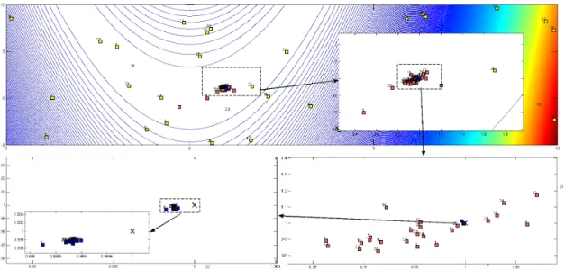
in the next chapter): initial population (by the squares signalized with yellow color); population at 15th generation (pink squares); and final population (blue squares).

Figure 3.1: Sequence of optimization process of DEEPSO for Rosenbrock’s function using a population of 30 paritcles. For the black and white prints, the lighter squares represent the initial population, the medium light represents 15th generation and the darknest squares concern to final population

As it can be observed, the initial population is randomly launched into search space within the limits placed. In a medium-scale view is already possible to observe a clear approach to the global minimum of this function, with the population at the fifteenth generation lies already in parabolic valley and distributed around the optimum point. Finally, by doing successive zooms on the details, there is the large majority of the final population distributed around the minimum point marked on (1,1) coordinates. The nearest particle of this point is at a module distance less than10−_{3 showing that the optimization process using the DEEPSO approach was successfully}

used for this test function.

As it was possible to show, the adaptive process incorporates the knowledge of the landscape, with a quick reduction in the initial dispersion through the alignment of particles along the valley, which incorporates the minimum of this function. This significant interaction found between the surroundings and each particle is due to the action of the selection operator, giving the feeling that the swarm can sense the type of landscape in which it is located.

This new heuristic method has shown great potential, suggesting to be even better than the EPSO. [16] Nonetheless, like EPSO, this new approach needs an adequate tuning of the following control parameters: mutation rate and communication factor.