A study of ensemble methods for vehicle classification on motorways

A study of ensemble methods for vehicle

classification on motorways

João Pedro Mendonça

DISSERTATION

R

Mestrado Integrado em Engenharia Informática e Computação Supervisor: Rosaldo J. F. Rossetti, PhD

Supervisor: Catarina Santiago, PhD

motorways

João Pedro Mendonça

Mestrado Integrado em Engenharia Informática e Computação

Computer Vision and Machine Learning are areas with many applications, with sensors based on the most diverse methods of image capture and video streaming being used more and more. From industrial processes to autonomous vehicles, from the identification of individuals to the moni-toring of cities, there are several applications.For the specific case of Intelligent Transportation Systems we are assisting to an increasing interest in such methodologies since highways are usu-ally equipped with cameras and so they can be used to perform in autonomous and automatic tasks such as: vehicle counting by class, incident detection, the identification of vehicles in irregularity, among others.

We are now faced with the consequences of numerous traffic occurrences, with negative implica-tions to both businesses and citizens. This results from an ineffective and subjective traffic control system, carried out by records conditioned by environmental factors, among which the quality of the image, the intensity of light, noise caused by the conditions of available light, camera position-ing, occlusion of objects and the subjectivity of human reasoning.

In this dissertation we applied an ensemble learning architecture for classifying vehicles. We propose a Bagging architecture with You Only Look Once, Single Shot MultiBox Detector and Background Subtraction as level 0 classifiers. To combine the output of the algorithms we imple-mented 2 options, namely: a Majority Voting algorithm and an Avg Best algorithm. In order to validate the proposed solution, the ensemble of classifiers was tested on three different highway datasets with different characteristics (size of the vehicles, angle of view, number of lanes and different number of classes, different lighting scenarios).

The proposed ensemble solution detected and classified more vehicles than any singular classifi-cation algorithm on 5 out of 6 tests. Single Shot MultiBox Detector proved very stable regardless of the test scenarios while You Only Look Once proved to have a better generalization with less samples of a class. Background Subtraction detects the fewest vehicles but classifies those objects almost as well as the other algorithms with faster prediction times.

Keywords:

Computing methodologies→ Computer-Vision

Computing methodologies → Machine learning → Machine learning approaches → Neural networks

Computing methodologies → Machine learning → Machine learning algorithms → Ensem-ble methods

Visão computacional e aprendizagem máquina são áreas com inúmeras aplicações, com sensores baseados nos mais diversos métodos de captura de imagem e streaming de vídeo sendo cada vez mais usados. De processos industriais a veículos autônomos, desde a identificação de indivíduos até à monitorização de cidades. Para o caso específico da área dos Sistemas Inteligentes de Trans-porte estamos a assistir a um interesse crescente em tais metodologias, já que as vias rodoviárias são geralmente equipadas com câmeras e elas podem ser usadas para executar tarefas autônomas e automáticas como: contagem de veículos por classe, detecção de incidentes, identificação de veículos em irregularidades, entre outros.

Somos agora confrontados com as consequências de numerosas ocorrências de tráfego, com im-plicações negativas para as empresas e para os cidadãos. Isto é o resultado de um sistema de controle de tráfego ineficaz e subjetivo, realizado por registos condicionados por fatores ambi-entais, de entre os quais figuram a qualidade da imagem, a intensidade da luz, o ruído provocado pelas condições de luz disponível, posicionamento da câmera, oclusão de objetos e a subjetividade do raciocínio humano.

Nesta dissertação aplicámos uma arquitetura de ’Ensemble Learning’ para classificar veículos. Propomos uma arquitetura de ’Bagging’ com ’You Only Look One’, ’Single Shot MultiBox De-tector’ e Subtração de Fundo como classificadores de nível 0. Para combinar a saída dos algorit-mos, implementámos 2 opções: um algoritmo de votação maioritária e um algoritmo de melhor média. Para validar a solução proposta, o conjunto de classificadores foi testado em três diferentes conjuntos de dados de rodovias com diferentes características (dimensão dos veículos, ângulo de visão, número de faixas, número de classes diferentes e diferentes cenários de iluminação). A solução proposta detectou e classificou mais veículos do que qualquer algoritmo de classificação singular em 5 de 6 testes. Single Shot MultiBox Detector mostrou-se muito estável, independente-mente dos cenários de teste, enquanto ’You Only Look Once’ provou ter uma melhor generaliza-ção com menos amostras de uma classe. Subtrageneraliza-ção de Fundo detecta o menor número de veículos, mas classifica esses objetos quase tão bem quanto os outros algoritmos com tempos de previsão considerávelmente mais rápidos.

My sincere thanks to Professor Rosaldo Rossetti and Catarina Santiago for all the support and guidance during the writing of this thesis. I also thank them for all the lessons that they taught me and that will stay with me throughout to the next challenges of my life. Also a thanks to Joel Carneiro for brainstorming help and for sharing his experience of his dissertation.

1 Introduction 1

1.1 Motivation . . . 1

1.2 Problem Definition . . . 2

1.3 Objectives and Contributions . . . 2

1.4 Document Structure . . . 2 2 Literature Review 3 2.1 Methods . . . 3 2.1.1 Detection . . . 5 2.1.2 Classification . . . 13 2.1.3 Ensemble Learning . . . 17

2.1.4 Metrics for Evaluating Classification Algorithms . . . 20

2.2 Related Work . . . 23

2.2.1 Detection and Classification . . . 23

2.2.2 Ensemble Learning . . . 25 2.2.3 Previous Approaches . . . 26 2.3 Summary . . . 26 3 Methodological Approach 29 3.1 Scope . . . 29 3.2 Support Technologies . . . 29 3.3 Proposed Solution . . . 30 3.3.1 Existing Solution . . . 30

3.3.2 Proposed System Architecture . . . 32

3.4 Summary . . . 40 4 Results 41 4.1 Dataset Specifications . . . 41 4.1.1 Dataset 1 . . . 42 4.1.2 Dataset 2 . . . 42 4.1.3 Dataset 3 . . . 44 4.2 Test Procedures . . . 45 4.3 Test Results . . . 46 4.4 Summary . . . 63 5 Conclusions 67 5.1 Further Developments . . . 68 5.2 Future Work . . . 69

5.3 Final Remarks . . . 69

2.1 CNN fully connected . . . 4 2.2 CNN example of architecture . . . 4 2.3 Softmax function . . . 4 2.4 RCNN overview . . . 6 2.5 Fast R-CNN architecture . . . 7 2.6 Faster R-CNN overview . . . 7 2.7 FPN explanation . . . 8 2.8 R-FCN architecture . . . 9 2.9 Overfeat architecture . . . 10

2.10 YOLO simple overview . . . 11

2.11 SSD pipeline architecture . . . 11

2.12 YOLOv3 prediction output and architecture . . . 12

2.13 RetinaNet architecture . . . 13

2.14 LDA explanation . . . 14

2.15 SVM example . . . 14

2.16 HMM example . . . 15

2.17 KNN example . . . 16

2.18 Decision Trees explanation . . . 16

2.19 Perceptron and multilayer perceptron . . . 17

2.20 Explanation of ensemble . . . 17

2.21 Stacking example . . . 18

2.22 Bagging example . . . 19

2.23 Boosting example . . . 20

2.24 AUC example . . . 22

2.25 Detection and Classification pipeline of [B. Coifman, 1998] . . . 24

2.26 Overview of [P. Barcellos, 2014] method for classifying vehicles . . . 25

3.1 Pre-existing pipeline to improve on . . . 31

3.2 Proposed system architecture with best average . . . 32

3.3 Proposed system architecture with majority voting . . . 33

3.4 SSD basic architecture . . . 34

3.5 Inception theory . . . 34

3.6 Background Subtraction work flow . . . 36

3.7 Regions where Background Subtraction classifies for dataset 1 . . . 36

3.8 Regions where Background Subtraction classifies for dataset 2 . . . 37

3.9 Regions where Background Subtraction classifies for dataset 3 . . . 37

4.1 Definition of data division . . . 41

4.2 Frame for training with a heavy vehicle of dataset 1 . . . 42

4.3 Frame for training with a light vehicle of dataset 2 . . . 42

4.4 Frame for training with a motorcycle and lightweight vehicles of dataset 2 . . . . 43

4.5 Frame for training with a heavy vehicle of dataset 2 . . . 44

4.6 Frame for training with a light vehicle of dataset 3 . . . 45

4.7 Example prediction of SSD for dataset 1 . . . 47

4.8 Example of prediction of YOLO for dataset 1 . . . 47

4.9 Example of prediction of Background Subtraction for dataset 1 . . . 48

4.10 Example of resulting Majority voting prediction for dataset 1 . . . 48

4.11 Example prediction of SSD for dataset 2 . . . 49

4.12 Example prediction of YOLO for dataset 2 . . . 50

4.13 Example prediction of Background Subtraction for dataset 2 . . . 51

4.14 Example prediction of Majority Voting for dataset 2 . . . 52

4.15 Example of prediction of SSD for dataset 3 . . . 53

4.16 Example of prediction of YOLO for dataset 3 . . . 54

4.17 Example of Majority Voting combination algorithm for dataset 3 . . . 55

4.18 Example of prediction of SSD trained on all the datasets for dataset 1 . . . 56

4.19 Example of prediction of YOLO trained on all the datasets for dataset 1 . . . 56

4.20 Example of prediction of Background Subtraction for dataset 1 . . . 57

4.21 Example of prediction of Majority voting combination for dataset 1 . . . 57

4.22 SSD prediction for heavy vehicle for error in combination . . . 58

4.23 YOLO incorrect prediction . . . 58

4.24 Final wrong prediction of the ensemble . . . 58

4.25 Example of prediction of SSD trained on all the datasets for dataset 2 . . . 59

4.26 Example of prediction of YOLO trained on all the datasets for dataset 2 . . . 60

4.27 Example of prediction of Background Subtraction for dataset 2 . . . 60

4.28 Example of prediction of Best Avg combination for dataset 2 . . . 60

4.29 Example of prediction of SSD for dataset 3 trained with all cameras . . . 61

4.30 Example of prediction of YOLO for dataset 3 trained with all cameras . . . 62

4.31 Example of prediction of Background Subtraction trained for dataset 3 . . . 62

4.32 Example of prediction of Majority Voting trained with all cameras for dataset 3 . 62 4.33 Summarized graphic for total boxes correct detections and classifications for each dataset . . . 63

4.34 Summarized graphic for detection performance per dataset . . . 64

4.35 Summarized classification performance . . . 64

4.36 Total boxes correct detections and classifications per each test set for training with all datasets . . . 64

4.37 Detection Performance per test set trained with all the datasets . . . 65

2.1 Example of a confusion matrix, TP means True Positive, FN means False Nega-tive, FP means False Positive and TN True NegaNega-tive, these concepts will be

ex-plained further and used in the next metrics . . . 21

3.1 Architecture of YOLO tiny . . . 35

4.1 training dataset on the left testing set on the right . . . 45

4.2 Evaluation Set 1 Results . . . 46

4.3 Evaluation Set 2 . . . 49

4.4 Evaluation Set 3 . . . 53

4.5 Evaluation Set 1 trained with all the cameras: 3145 boxes, 124 light and 21 heavy vehicles . . . 56

4.6 Evaluation Set 2 trained with all the cameras: 3782 boxes, 68 light vehicles, 12 heavy vehicles and 1 motorcycle . . . 59

4.7 Evaluation Set 3 trained with all the cameras: 512 boxes, 60 light vehicles and 17 heavy vehicles . . . 61

SSD Single Shot Multi-box Detector YOLO You Only Look Once

ITS Intelligent Transport System CNN Convolutional Neural Network R-CNN Regions with Convolutional Features mAP mean Average Precision

RoI Regions of Interest

RPN Region Proposals Networks FPN Feature Pyramid Networks

R-FCN Region based Fully Convolutional Networks SVM Support Vector Machine

LDA Linear Discriminant Analysis HMM Hidden Markov Model KNN K-Nearest Neighbour AUC Area Under the Curve

OpenCV Open Source Computer Vision Library TPU Tensor Processing Unit

Introduction

1.1

Motivation

Computer Vision and Machine Learning are areas with many applications, with sensors based on methods of image capture and video streaming being used more and more. The result has many uses: the counting of vehicles by class, the detection of incidents, the identification of vehicles in irregularity, among others.

At ARMIS ITS (Intelligent Transport System) they apply information and communication tech-nologies to the transport area, through intelligent solutions that reduce accidents, CO2 emissions and improve traffic conditions, ensuring values such as sustainability, efficiency and safety. ARMIS has been working on the area of detection and tracking of vehicles and currently has a solution. This suggests that the company might have an interest in the findings of this thesis in the ITS area.

According to [Toroyan, 2015] more than 1.2 million people die each year on the world’s roads, making road traffic injuries a leading cause of death globally. In [ITS, 2018] "The ITS market in roadways is expected to be worth USD 23.35 billions in 2018 and USD 30.74 billions by 2023, at a Compound Annual Growth Rate (CAGR) of 5.65% between 2018 and 2023." This increase is attributed to an increase in traffic congestion, concerns of public safety and government initiatives for effective and modern traffic management. In the Portuguese landscape, some news also con-firm the interest of government infrastructures in modern traffic management systems as reported in [Lusa, 2018] which shows also a positive approach to the area and the environment in which our problem is inserted since the input video data used in this work will be from the Porto area. Currently counting of vehicles is done manually, where humans classify vehicles while watching the video so there is also the motivation to ease the work for humans but not necessarily relieving them from the process entirely.

1.2

Problem Definition

Current approaches to classifying vehicles on highways with a single model have lead to inconsis-tencies in the results, as some methods overfit on the training set and do not classify some of the vehicles of the test set.

1.3

Objectives and Contributions

With this dissertation, we intend to feature traffic management systems with intelligent function-alities, using computer vision algorithms. Some video cameras from Portuguese highways will be used for the implementation, proof of concept and tests of the classification algorithms by com-puter vision.

The objectives defined for this thesis are the following:

1. achieve a more accurate output than single model prediction 2. show from each model the features that get valued the most

1.4

Document Structure

The next section, Literature Review, is divided in two parts, namely the methods part that provides an overview of the algorithms that are mostly used on the context of this thesis problem and the second part, Related Work, where the related solutions are described.

In the third chapter, Methodological Approach, our solution to the problem is explained with the scope, proposed solution details and support technology.

In the fourth chapter, we present the Test Procedures and Results as well as a description of each dataset and the implications of each. The fifth and final chapter includes the conclusions and provides some guidelines for future work.

Literature Review

This chapter attempts to be a two part guide. The first part presents a guide to algorithms for De-tection and Classification, methods for combining different classification algorithms and metrics for evaluating them. The first attempts featured approaches based on detection and classification in separate phases while newer applications do detection and classification at the same stage. The second part presents a review of what has been done in the area of vehicle detection, classification and ensemble systems.

2.1

Methods

In order to understand more recent approaches to detection, we must first know what is a CNN, a convolutional neural network, this explanation is based on [A. Krizhevsky, 2012] and [Y. Lecun, 2015]. A CNN takes four steps: convolution, Pooling, Flattening and Full connection.

Convolution is a mathematical operation that multiplies two functions (dot product) creating a third that expresses how one influences the other, on the case of computer vision, convolution is a small filter that goes through the entire image computing the dot product between the entries of the filter and the input image. A network is convolutional if it has at least a convolutional layer that builds feature maps from the input image.

Pooling reduces the complexity, by reducing the number of bytes taken from the feature map by using a mask. Flattening transforms the pooling maps into an input layer for the network. Full connection means that every neuron in a layer is connected to all the neurons in the immediate previous and immediate next layers. From here a CNN is just like any Neural Network it has an input layer, some hidden layers that compute weights based on training and an output layer that provides a prediction.

Figure 2.1: Taken from Udemy paid course about Deep Learning[Eremenko, 2018] Example of a CNN in the fully connection step.

Figure 2.2: Taken from [A. Krizhevsky, 2012] Example of architecture of a CNN

Some CNNs, as presented next, use Softmax functions for the output of predictions. As ex-plained more thoroughly in[Nasrabadi, 2007], Softmax is a function that takes a K-dimensional vector z and transforms it into a K-dimensional vector of real values, where each entry is in the range [0, 1].

The final concept to understand is logistic regression that to put it very simple is what allows for an approximation to a binary result, pass or fail, based on the value it either outputs 0 or 1.

2.1.1 Detection

Detection is the method in which key-points or groups of key-points, are qualified according to an objective, in the case of object detection in which vehicle detection is a part of, the method focuses on finding groups of key-points to determine where there are objects. In 2003 the Scale Invariant Feature Transform(SIFT) was presented in the "Distinctive Image Features from Scale-Invariant Keypoints" paper, [Lowe, 2004]. This technique consisted in four stages: first a search over all scales and image regions finding the candidate points; second, for each candidate region, a model is used to determine location and scale of keypoints; third at least one orientation is assigned to each keypoint location using image gradient directions; fourth image gradients are measured at the selected scale in the region around each keypoint.

From here on a lot of different methods came to light, as of late detection algorithms that integrate classification with detection have been heating up. Currently three types of detectors exist as cate-gorized in [T.-Y Lin, 2018] and will be explained resorting to examples: Classic Object Detectors, Two-stage Detectors and One-stage Detectors.

2.1.1.1 Classic Object Detectors

Classic Object Detectors consist in a classifier being applied to a dense image grid. Yann Lecun regarded as the father of Convolutional Neural Networks (CNN), is responsible for the earliest

im-plementation by applying a classifier (CNN) on handwritten digit recognition.[Y. LeCun, B. Boser, J. S. Denker, D. Henderson, R. E. Howard, W. Hubbard, L. D. Jackel, 1990] Even though sliding window methods were mostly used in object detection as said in [T.-Y Lin, 2018],

the revival of deep learning allowed the appearance of two other types of detectors Two-Stage and One-Stage detectors.

2.1.1.2 Two-Stage Detectors

As the name indicates, two-stage dectetors are composed by two stages, the first stage, detects and the second classifies. Two stage detectors came to dominate the paradigm, in the first phase the set of candidate locations (locations of images with a probable image in it) get generated, this separates most of the non object locations from the object locations (99%), in the second phase the set of candidates get classified into background and foreground. The first to use this methodology were [J. Uijlings, 2013] in Selective Search paper and upgraded upon the launch of R-CNN[R. Girshick, 2014] with a convolutional neural network (CNN) for for the second phase classification which brought with it an increase of accuracy.

The R-CNN [R. Girshick, 2014] abbreviation comes from the use of Region proposal with a CNN. The technique is composed by three modules, the first generates category-independent region proposals. These proposals define the set of candidate detections available to the detector. The second module is a large convolutional neural network (CNN) that extracts a fixed-length feature vector from each region. The third module is a set of class-specific linear Support Vector machines (SVMs).

Figure 2.4: Taken from [R. Girshick, 2014] Object detection system overview. System (1) takes an input image, (2) extracts around 2000 bottom-up region proposals, (3) computes features for each proposal using a large convolutional neural network (CNN), and then (4) classifies each region using class-specific linear SVMs

After the R-CNN, an improvement was made called the fast R-CNN[Girshick, 2015] that fea-tured a new trained network that was faster at test time and more accurate (mAp). Furthermore, training became single stage using a multi-task loss. The network first processes the whole image with several convolutional and max pooling layers to produce a convolutional feature map. Then, for each object proposal a region of interest pooling layer extracts a fixed-length feature vector from the feature map. Each feature vector is fed into a sequence of fully connected layers that finally branch into two sibling output layers: one that produces softmax probability estimates over K object classes (the number of classes of objects) plus a catch-all “background” class and an-other layer that outputs four real-valued numbers for each of the K object classes, those values are encoded refined bounding box positions.

Figure 2.5: Taken from [Girshick, 2015] Fast R-CNN architecture. An input image and multiple regions of interest (RoIs) are input into a fully convolutional network. Each RoI is pooled into a fixed-size feature map and then mapped to a feature vector by fully connected layers (FCs). The network has two output vectors per RoI: softmax probabilities and per-class bounding-box regression offsets. The architecture is trained end-to-end with a multi-task loss

Upgrades to Fast R-CNN have been made in the past few years with learned object proposals and Region Proposals Networks (RPN) like the faster R-CNN [S. Ren, 2015] where a RPN takes an image (of any size) as input and outputs a set of rectangular object proposals, each with an objectness score (probability of being an object), an RPN is a fully convolutional network that simultaneously predicts object bounds and objectness scores at each position. RPNs are trained end-to-end to generate high-quality region proposals. The Faster R-CNN is an upgrade using the aforementioned RPN that shares full image convolutional features with the detection network. Ex-tensions and small upgrades have been made more recently.

Figure 2.6: Taken from [S. Ren, 2015] Left: Region Proposal Network (RPN). Right: Example detections using RPN proposals on PASCAL VOC 2007 test. This method detects objects in a wide range of scales and aspect ratios

Feature Pyramid Networks for Object Detection is one of those extensions to faster R-CNN[T.-Y Lin, 2017] where these pyramids are scale-invariant in the sense that an object’s scale change is offset by

shift-ing its level in the pyramid. Intuitively, this property enables a model to detect objects across a large range of scales by scanning the model over both positions and pyramid levels.

Figure 2.7: Taken from [T.-Y Lin, 2017]Figure 1. (a) Using an image pyramid to build a feature pyramid. Features are computed on each of the image scales independently, which is slow. (b) Recent detection systems have opted to use only single scale features for faster detection. (c) An alternative is to reuse the pyramidal feature hierarchy computed by a ConvNet as if it were a featurized image pyramid. (d) their proposed Feature Pyramid Network (FPN) is fast like (b) and (c), but more accurate. In this figure, feature maps are indicated by blue outlines and thicker outlines denote semantically stronger features

Another extension is R-FCN [Y. Li, 2016] following R-CNN, R-FCN adopts the two-stage ob-ject detection strategy that consists of: (i) region proposal, and (ii) region classification. It extracts candidate regions by the Region Proposal Network [S. Ren, 2015] and as described above which is a fully convolutional architecture in itself. The approach shares the features between RPN and R-FCN. The figure2.8this text shows an overview of the system.

Given the proposal regions (RoIs), the R-FCN architecture is designed to classify the RoIs into object categories and background. In R-FCN, all learnable weight layers are convolutional and are computed on the entire image. The last convolutional layer produces a bank of k2 position-sensitive score maps for each category, and thus has a k2(C + 1)-channel output layer with C object categories (+1 for background). The bank of k2 score maps correspond to a k × k spatial grid de-scribing relative positions. R-FCN ends with a position-sensitive RoI pooling layer. This layer aggregates the outputs of the last convolutional layer and generates scores for each RoI.

Figure 2.8: Taken from [Y. Li, 2016] Overall architecture of R-FCN. A Region Proposal Network (RPN)[S. Ren, 2015] proposes candidate RoIs, which are then applied on the score maps. All learnable weight layers are convolutional and are computed on the entire image;

2.1.1.3 One-Stage Detectors

One-stage detectors have existed for some time, Overfeat [P. Sermanet, 2014] has kick-started newer developments as one of the first one-Stage detectors, using a single CNN to detect, classify, locate in that order and using a shared feature learning base. In Classification, each image is as-signed a single label corresponding, to the main object in it, it uses five guesses to find the correct labeling. In Localization a bounding box for the predicted object is returned with each of the five guesses. In Detection the task differs from localization because there can be any given number of objects in the image (even zero) and false positives are penalized by mean average precision measure (mAP).

Figure 2.9: Taken from [P. Sermanet, 2014]Localization (left top) and detection tasks (left bot-tom). The most left images contain predictions (ordered by decreasing confidence) while the left right images show the groundtruth labels. The detection image (left bottom ) illustrates the higher difficulty of the detection dataset, which can contain many small objects while the classification and localization images typically contain a single large object. To the right the images are Layer 1 filters (right top) of features and the layer 2 filters (right bottom)

Recently the interest in creating a fast detector to allow real time detection has brought new

de-velopments of accuracy and speed. Like YOLO [J. Redmon, 2015,J. Redmon, 2018], SSD[W. Liu, 2016], RetinaNet [T.-Y Lin, 2018].

YOLO, meaning You Only Look Once, uses a regression problem approach (classification aims at predicting a label while regression is about predicting a quantity) to spatially separate bounding boxes and object class probabilities using a single CNN in a single evaluation of a full image as written in [J. Redmon, 2015].

Figure 2.10: Taken from [J. Redmon, 2015]YOLO divides the image into an S × S grid and for each grid cell predicts B bounding boxes, confidence for those boxes, and C class probabilities

SSD as described in [W. Liu, 2016], splits the output bounding boxes into a set of default boxes per different image ratios, scales and per feature map location. During prediction time the algorithm’s network scores the presence of each object category in each default box and produces adjustments to the box more closely match the object shape. Additionally, the network combines predictions from multiple feature maps with different resolutions to naturally handle objects of various sizes.

Figure 2.11: Taken from [W. Liu, 2016]SSD framework. (a) SSD only needs an input image and ground truth boxes for each object during training. In a convolutional fashion, it evaluates a small set of default boxes of different aspect ratios at each location in several feature maps with both the shape offsets and the confidences for all object categories ((c1, c2, · · · , cp)) different scales (e.g. 8 × 8 and 4 × 4 in (b) and (c)). For each default box, it predicts At training time, the algorithm first matches these default boxes to the ground truth boxes. For example, if there has been matched two default boxes with the cat and one with the dog, which are treated as positives and the rest as negatives. The model loss is a weighted sum between localization loss and confidence loss (e.g. Softmax).

Recently, a third updated version of YOLO, YOLOv3 [J. Redmon, 2018], was released. In this version YOLO predicts bounding boxes using dimension clusters as anchor boxes. The network predicts 4 coordinates for each bounding box and then predicts an objectness score for each bound-ing box usbound-ing logistic regression. Each box predicts the classes in the boundbound-ing box. YOLOv3 predicts boxes at 3 different scales, system extracts features from those scales using a similar con-cept to feature pyramid networks (FPN). Then they take the feature map from 2 layers previous and upsample it two times. They also take a feature map from earlier in the network and merge it with upsampled features using concatenation to get more meaningful semantic information from the upsampled features and finer-grained information from the earlier feature map. A new net-work for feature extraction was also created and trained, it was called Darknet 53, because of it’s 53 convolutional layers. In this version there is also a smaller version of yolo, tiny-yolo which is extremely fast in training, the architecture is similar but with less convolutional layers.

Figure 2.12: Taken from [J. Redmon, 2018]Left:Bounding boxes with dimension priors and loca-tion predicloca-tion. Predicts the width and height of the box as offsets from cluster centroids. Predicts the center coordinates of the box relative to the location of filter application using a sigmoid func-tion. Right:Architecture of the convolutional neural network Darknet-53

RetinaNet, or as the paper is called, Focal Loss for Dense Object Detection [T.-Y Lin, 2018], is the final detector in this chapter and the second most recent one. RetinaNet is a single, uni-fied network composed of a backbone network and two task-specific subnetworks. The backbone is responsible for computing a convolutional feature map over an entire input image. The first subnet performs convolutional object classification on the backbone’s output; the second subnet performs convolutional bounding box regression. They built a FPN[T.-Y Lin, 2017] on top of the ResNet[K. He, 2016] as the backbone network the pyramid has levels P3 through P7, where l indicates pyramid level (Pl has resolution 2l lower than the input). Preliminary experiments us-ing features from only the final ResNet[K. He, 2016] layer yielded low AP. The algorithm uses translation-invariant anchor boxes similar to those in the RPN variant in FPN [T.-Y Lin, 2017].

The anchors have areas of 322to 5122on pyramid levels P3 to P7, respectively.

The classification sub-network predicts the probability of object presence at each spatial position for each of the A anchors and K object classes. This subnet is a small FCN (fully convolutional network) attached to each FPN level; parameters of this subnet are shared across all pyramid lev-els. It is designed to taking an input feature map with C channels from a given pyramid level, the subnet then applies four 3 × 3 conv layers, each with C filters and each followed by ReLU acti-vations, followed by a 3 × 3 conv layer with KA filters. Finally sigmoid activations are attached to output the KA binary predictions per spatial location. In parallel with the object classification subnet, another small FCN is attached to each pyramid level for the purpose of regressing the off-set from each anchor box to a nearby ground-truth object.

Figure 2.13: Taken from [T.-Y Lin, 2018] The one-stage RetinaNet network architecture uses a Feature Pyramid Network (FPN) backbone on top of a feedforward ResNet[K. He, 2016] archi-tecture (a) to generate a rich, multiscale convolutional feature pyramid (b). To this backbone RetinaNet attaches two subnetworks, one for classifying anchor boxes (c) and one for regressing from anchor boxes to ground-truth object boxes (d). The network design is intentionally simple, which enables this work to focus on a novel focal loss function that eliminates the accuracy gap between the one-stage detector and state-of-the-art two-stage detectors like Faster R-CNN with FPN

2.1.2 Classification

Current object detectors based on neural networks already integrate classification with detection but for the purpose of presenting a bigger picture, many classification algorithms will be presented here, not only neural networks.

2.1.2.1 Linear Discriminant Analysis(LDA)

LDA’s aims at utilizing hyperplanes to split the different classes. To do that it is necessary to find the expression of a plane that maximizes the distance between two classes and minimizes the interclass variance. The more classes the more planes are necessary to separate each of the classes from the others.

Figure 2.14: taken from [F. Lotte, 2007] A hyperplane which separates two different classes 2.1.2.2 Support Vector Machines(SVM)

SVM is a supervised learning algorithm that just like LDA the idea is to also define a hyperplane to separate classes but the most important criterion is the maximum margin hyperplane.

Figure 2.15: taken from [F. Lotte, 2007] the optimal hyperplane for generalization 2.1.2.3 Hidden Markov Model(HMM)

The mindset of Hidden Markov Model is to compute in the best way, given the parameters of the model, the probability of a particular output sequence. This requires summation over all possible state sequences. Each state of the automaton can estimate the probability of observing a given feature vector.

Figure 2.16: taken from [E. Sonnhammer, 1998] The structure of the model used in TMHMM(Transmembrane Helix Hidden Markov Model). A) The overall layout of the model. Each box corresponds to one or more states. Parts of the model with the same text are tied, i.e. their parameters are the same. Cyt. means the cytoplasmic side of the membrane and non-cyt. the other side. B) The state diagram for the parts of the model denoted helix core in A. From the last cap state there is a transition to core state number 1. The first three and the last two core states have to be traversed, but all the other core states can be bypassed. This models core regions of lengths from 5 to 25 residues. All core states have tied amino acid probabilities. C) The state structure of globular, loop, and cap regions. In each of the three regions the amino acid probabilities are tied. The three different loop regions are all modelled like this, but they have different parameters in some regions

2.1.2.4 K Nearest Neighbor classification(KNN)

KNN is based on the input of the k closest training sets in the feature space. An object is classified by a majority vote of its neighbors and k is the number of neighbors that vote to classify that object. The object is assigned to the class most common among its k nearest neighbors. If k = 1, then the object is simply assigned to the class of that single nearest neighbor. The bigger the k the lesser the noise, but also there is a risk of less separation between classes.

Figure 2.17: Example of K-Nearest Neighbours [P. Cunningham, 2007] 2.1.2.5 Decision trees

A Decision Tree is a diagram where each branch represents a test or as it is called in [Aggarwal, 2014] a split criterion, whose objective is to try splitting the training data in order to maximize the dis-crimination among the different classes over different nodes.

Figure 2.18: taken from [Aggarwal, 2014] Univariate is when the criterion is on a single attribute. Multivariate is when the split criterion uses conditions on multiple attributes.

2.1.2.6 Neural networks

In the start of this chapter a type of neural networks, the convolutional neural networks, were described to serve as introduction to the detection section.

In the book ”Data classification: algorithms and applications” [Aggarwal, 2014] the author states: ”Neural networks attempt to simulate biological systems, corresponding to the human brain. In the human brain, neurons are connected to one another via points, which are referred to as synapses. In biological systems, learning is performed by changing the strength of the synaptic connections, in response to impulses.” In computer science, Neural networks are supervised learning method composed by a group of layers of neurons, an input layer and an output layer. Each of those

neurons on the output layer get the information that was inserted in the input layer with some weights associated, those weights are the strength of the synapses. It is by adjusting the weights associated with each input that the algorithm "learns" how each part of the data influences the output classification.

Figure 2.19: taken from [Aggarwal, 2014] Perceptron and Multilayer Perceptron 2.1.3 Ensemble Learning

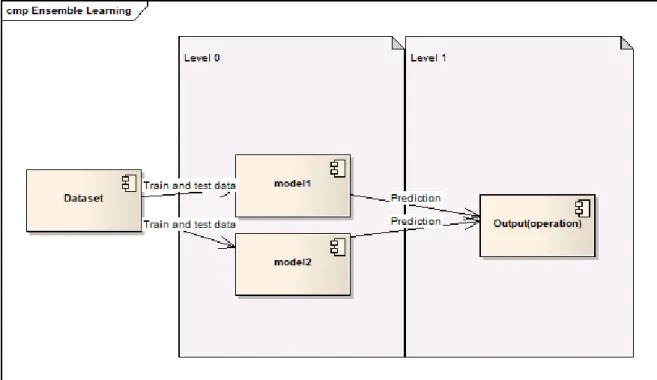
Ensemble Learning consists in combining predictions of multiple different models to increase per-formance. Some of these techniques are described next based on what was found in [Polikar, 2006] and [M. Galar, 2011]. As a matter of introduction, three very simple ensemble methods exist: max voting, averaging and weighted average.

Figure 2.20: Example diagram to explain the most basic idea of Ensemble learning. In figure2.20a dataset is used to train and test the models in the level 0 then the output of the models gets fed forward to an operation or another model in the next level, this is the most basic

idea behind ensemble.

Starting with max voting the output operation in the example is the mode of the predictions from the models. In weighted average each model gets an associated weight based on importance and the weighted average gets calculated as this (p1 ∗ w1 + p2 ∗ w2)/2 where p1 is the prediction of model1 and w1 is the weight given to model1. The average method implies the calculation of the normal average to combine the outputs. Other more advanced approaches are Stacking, Bagging and Boosting.

2.1.3.1 Stacking

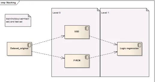
Stacking is an ensemble learning technique that takes predictions from multiple models to build a new model and then that model outputs the final predictions on the test set. The train set is used for the training of the level 0 models and for their predictions as well, those predictions are then used to build the next level model.

Figure 2.21: In this example SSD and F-RCN are the models of level 0, they make the predictions on the train set and those predictions are used to build the Logistic Regression model in level1 that makes predictions on the original test set

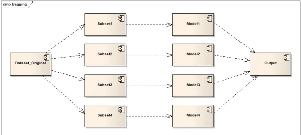
2.1.3.2 Bagging

Bagging or bootstrap aggregation consists in creating subsets from the original dataset and using each of these subsets to train different independent models. The predictions of each of these independent models are then combined using voting for classification or average.

Figure 2.22: four random subsets from the original data go through four independent models that output predictions. Those predictions are combined to make the final the output.

Bagging has two variations according to [Polikar, 2006]: Random forests and Pasting small votes. Random forests are created from decision trees with varying training parameters and said parameters can be bootstrapped versions of the train data or different feature subsets. Pasting small votes on the other hand uses large data partitioned into smaller subsets used to train different clas-sifiers, the data subsets can be created at random, called "Rvotes", or can be created consecutively based on importance of instances (those that improve diversity), called "Ivotes".

2.1.3.3 Boosting

The idea behind boosting is to use weak models (barely better than random guessing) by training them on small subsets and then make predictions on the whole dataset. The wrong predictions are weighted with bigger weights, then another model is created and fed the weighted data to attempt to correct the mistakes from the previous model this happens on a sequential loop with N iterations. The final model uses a weighted mean of all the weak models.

Figure 2.23: In the first iteration all the data has the same weight, a subset is sampled from the whole dataset. A model is trained on the subset and makes predictions on the whole dataset. The data that the model predicted incorrectly get higher weights and the cycle restarts with the updated data weights.

2.1.4 Metrics for Evaluating Classification Algorithms

Classification algorithms fall under the category of machine learning algorithms. The most com-mon metrics for machine learning algorithms are: Classification Accuracy, Logarithmic Loss, Confusion Matrix, Area under Curve, F1 Score, Mean Absolute Error and Mean Square Error.

2.1.4.1 Classification Accuracy

Classification Accuracy is the ratio between the correct predictions and total predictions. Accuracy = Number of Correct Predictions

Total Number of Predictions Made (2.1) It only evaluates well when there is the same amount of samples for each class.

2.1.4.2 Logarithmic Loss

The Logarithmic Loss metric penalizes the wrong classifications. It requires the classifier to assign a probability to each class. N samples, M classes, yi j indicates whether sample i belongs to class

jor not, pi j, indicates the probability of sample i belonging to class j

Logarithmic Loss = −1 N N

∑

∑

2.1.4.3 Confusion Matrix

A Confusion Matrix describes the performance in more detail. It looks at each of the predictions and the actual class. So it is easier to understand, [A. Mishra, 2018] has a very simple example:

Table 2.1: Example of a confusion matrix, TP means True Positive, FN means False Negative, FP means False Positive and TN True Negative, these concepts will be explained further and used in the next metrics

Predicted: Class1 Predicted: Class2 Actual: Class1 100 (TP) 10 (FN) Actual: Class2 5 (FP) 50 (TN)

What this means is that the algorithm predicted Class1 a hundred times and that was the actual class (TP), so the right prediction, fifty times predicted Class2 and it was the actual class (TN). The classification accuracy can be calculated from this since Number of Correct Predictions = 100 + 50 and the Total Number of Predictions Made = 100 + 5 + 10 + 50 so as written above

Accuracy= 150/165

2.1.4.4 Area Under the Curve(AUC)

AUC works well only with binary classification (where there is only Class1 or Class2) problems since it is the probability of the classifier ranking a random chosen positive higher than a random chosen negative. To define the AUC it is necessary to calculate True Positive Rate and False Positive Rate.

True Positive Rate = True Positive

False Negative + True Positive (2.3) False Positive Rate = False Positive

False Positive + True Negative (2.4) The area under the curve of plot False Positive Rate vs True Positive Rate is the AUC.

Figure 2.24: Example of an area under the curve taken from [J. Huang, 2005] A,B,C,D are classi-fiers

2.1.4.5 F1 Score

This metric evaluates how precise and robust the classifier is, the greater the value of F1 the better. F1 = 2 ∗ ₁ 1

precision+ 1 recall

(2.5)

Precision is the fraction of the Positives predicted that were correctly classified. Precision = True Positives

False Positives + True Positives (2.6) Recall is the fraction of actual Positives that existed and that the model predicted correctly.

Recall = True Positives

False Negatives + True Positives (2.7) High precision means that it is accurate, but lower recall means that misses too many of difficult to classify instances.

2.1.4.6 Mean Absolute Error

As the name says Mean Absolute Error is the mean of difference between the Actual Values and the Predicted Values it can also be described as the distance between the Values.

Mean Absolute Error = 1 N

N

∑

j=1

yjand y2j one represents the actual value for class j and the other the predicted for class j

2.1.4.7 Mean Squared Error

This metric is similar to the Mean Absolute Error except for the fact that it uses the square of the difference. The error gets squared so it becomes larger and more significant.

Mean Squared Error = 1 N

N

∑

j=1

(yj− y2j)2 (2.9)

yjand y2j one represents the actual value for class j and the other the predicted for class j

2.2

Related Work

In this section the current related solutions are explored. This is done to achieve better understand-ing of what has been done in the area and what technologies are indispensable for the work.

2.2.1 Detection and Classification

In 1998, an approach to a traffic surveillance system based on vehicle tracking called "A real-time computer vision system for vehicle tracking and traffic surveillance" [B. Coifman, 1998] was introduced. In this solution the authors proposed a feature-based tracking system for detecting ve-hicles under the challenging conditions. Instead of tracking entire veve-hicles, vehicle’s most salient features are tracked to make the system robust to partial occlusion. Leaving out the camera cali-bration that was done at that time, in the detection module corner features are defined as regions in the gray level intensity image where brightness varies in more than one direction. The corner features are tracked over time in the tracking module using Kalman filtering [Gelb, 1974] (using a mean weighted measure predicts the state of the system with a new value) to predict a given cor-ner’s location and velocity in the next frame. This approach is very old but the theoretical idea of feature based tracking is very good which will be thought for the tracking approach of our solution.

Figure 2.25: Taken from [B. Coifman, 1998] Overview of the system. To clarify the classification model was not implemented.

In 2008 the Institute of systems and Robotics of the FCT from the University of Coimbra Created a funded Project by Brisa [Monteiro, 2008] that included Robust Vehicle Segmentation, Stopped Vehicles Detection, Wrong Way Drivers Detection, Vehicle Counting, Vehicle Velocity Estimation project by Brisa. Describes a sliding window paradigm and it is not an integrated solu-tion since that project is more of an experiment of solving each sub-problem independently than to solve the three sub-problems of detection, classification and tracking, simply solves each problem separately together.

In 2015 [P. Barcellos, 2014] "A novel video based system for detecting and counting vehicles at user-defined virtual loops" was presented. As written in [P. Barcellos, 2014], the proposed method used motion coherence and spatial adjacency to group sampling particles in urban video sequences. A foreground mask is created using Gaussian Mixture Models and Motion Energy Images to determine the preferable locations that the particles must sample, and the convex particle groups are then analyzed to detect the vehicles. After a vehicle is detected, it is tracked using the similarity of its colors in adjacent frames. The vehicles are counted in user-defined virtual loops, by detecting the intersections of the tracked vehicles with these virtual loops.

Figure 2.26: Taken from [P. Barcellos, 2014] Overview of the method

This program however is still inefficient as it was written in [P. Barcellos, 2014]:"However, the proposed method may have a worse vehicle counting performance when the traffic flow is interrupted to be later resumed. Also, vehicle occlusions tend to worsen the vehicle counting per-formance of the proposed method. Small vehicles may be missed by the proposed method (...)" . Also since it is from 2015 none of the newer algorithms for detection and classification have been used.

Data from sky [Dat, 2018] uses aerial images to detect, classify and track providing the end user with detailed information like speed, counting and detecting anomalies. Uses drones to collect the video feed, does not use common traffic surveillance feeds. Only works with very high resolution aerial images and can not be used with current installation of cameras. There is not a paper or anywhere where to see the details of the implementation so the analysis is more on what features it provides and what requirements it has. This competing solution appears mentioned here as more of a curiosity of the applications since it can not be of use given that there is no information on the theory or implementation behind the product.

2.2.2 Ensemble Learning

"A Review on Ensembles for the Class Imbalance Problem: Bagging-, Boosting-, and Hybrid-Based Approaches", [M. Galar, 2011], is not a specific scenario where there was used a fusion of classifiers applied to vehicle classification, but actually it is focused on experiments done on many

different implementations of methods of ensemble but not in the field of vehicles specifically. Al-though there is a metric of accuracy of each algorithm tested on three vehicle datasets.

In these experiments each of the algorithms is compared with the other algorithms that are similar, belong to the same family, from there the better performing algorithms of each family are selected to be compared with the better performing algorithms of other families. The study provides some interesting conclusions, namely that ensemble based algorithms improve the results of single clas-sifiers, more complex methods do not outperform simpler ones and presents a good idea behind the experimentation method and which algorithms might be better.

In "Ensemble of Exemplar-SVMs for Object Detection and Beyond" [T. Malisiewicz, 2011], the author uses a bagging like ensemble approach to vehicle detection and classification even though it does not mention it as bagging. This approach featured an ensemble of SVMs trained on different vehicles.

Adaboost has been reported in uses for vehicle classification in a pipeline for rear view vehicle detection system based on monocular vision[Wang and Cai, 2015] and [Wen et al., 2015] where there is an approach to increasing Adaboost training speed for vehicle classification.

2.2.3 Previous Approaches

This work was done in Artificial Intelligence and Computer Science Lab Faculty of Engineering, University of Porto where there were already previous approaches in the ITS area we present some next: In ”Video Processing Techniques for Traffic Information Acquisition Using Uncontrolled Video Streams” [P. Loureiro, 2009], this paper presents a survey to the first attempts at monitoring transportation systems in order to provide information useful to the community. Adding to the survey there is an analysis of the issues that may arise and the best methods to solve them. In ” A computer-vision approach to traffic analysis over intersections” [G. Lira, 2016], this paper presents an approach using computer vision algorithms on videos obtained with drones of vehicles crossing intersections. This is done to identify and track vehicles, with the finality of extracting a statistical model.

In ”Computer-vision-based surveillance of intelligent transportation systems” [Neto et al., 2018], this paper describes the development of a video analytics server to detect and classify vehicles on motorways. This approach features Background Subtraction for detection and a fuzzy set for classification.

2.3

Summary

A lot of development has been done in the are of detection and classification, some was described in this chapter other has been left out since it was not in consideration for our solution. Some

solutions solve one problem and leave another unsolved, some are faster but with worse accuracy, others the opposite. Some methods require more data, others require weak learners but more com-putational power. The metrics vary, a few only work for binary classification problems while the others can be applied to anything, a combination of many is the best way to evaluate the classifi-cation.

Even though many similar applications have been made there is still space for further devel-opments in order to improve the solutions by using different algorithms and different approaches.

Methodological Approach

As written in the first chapter, our problem is to solve inconsistencies of single model predictions when classifying vehicles on highways. From this problem a set of questions have emerged:

1. Which algorithms classify vehicles better on their own?

2. How to fix the inconsistencies of single models to achieve a better result of classification?

3.1

Scope

Scope is defined as either Project Scope or Product scope.

According to [Kerzner, 2017], the work that needs to be accomplished to deliver a product, ser-vice, or result with the specified features and functions (hows) compose the project scope. Also according to [Kerzner, 2017], the features and functions that characterize a product, service or result (whats) is the product scope.

At first, the isolated classification algorithms will be evaluated in order to assess their strong and weak points. Afterwards, based on the findings, create an hypothesis that defines which al-gorithms will be used to solve which problems and what are their constraints. Finally solve the problem using that hypothesis.

The product scope associated is to deliver a module integrated on the existing pipeline with the fusing of different classifying algorithms allowing to see the independent accuracy of each algorithm and the combined predictions as output. These are the two scopes that can be defined in this work.

3.2

Support Technologies

Taken from [OpenCV, 2018],OpenCV (Open Source Computer Vision Library) is an open source computer vision and machine learning software library. OpenCV was built to provide a common

infrastructure for computer vision applications and to accelerate the use of machine perception in the commercial products. Being a BSD-licensed product, OpenCV makes it easy for businesses to utilize and modify the code.

As it can bee found in [Ten, 2018], TensorFlowTMis an open source software library for high performance numerical computation. Its flexible architecture allows easy deployment of compu-tation across a variety of platforms (CPUs, GPUs, TPUs), and from desktops to clusters of servers to mobile and edge devices. Originally developed by researchers and engineers from the Google Brain team within Google’s AI organization, it comes with strong support for machine learning and deep learning and the flexible numerical computation core is used across many other scientific domains.

Taken from [Chollet, 2015], Keras is a high-level neural networks API, written in Python and capable of running on top of TensorFlow, CNTK [CNT, 2017], or Theano [The, 2017]. It was developed with a focus of enabling fast experimentation. Being able to go from idea to result with the least possible delay is key to doing good research. Allows for easy and fast prototyping (through user friendliness, modularity, and extensibility). Supports both convolutional networks and recurrent networks, as well as combinations of the two. Runs seamlessly on CPU and GPU.

The scikit-learn [sci, 2017] provides API to calculate metrics like F1, accuracy, AUC and other algorithms for optimization.

3.3

Proposed Solution

In the next sections we will first analyze the existing solution and then we will present the proposed changes to that solution. It is important to analyze the existing solution in order to find what can be done to improve it.

3.3.1 Existing Solution

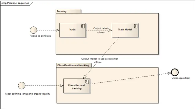
Figure 3.1: Basic Implementation pipeline

This pipeline comprises training and annotation of videos that can serve as dataset.

The tensorflow object detection pipeline for training [Ten, 2018] is used for the neural network classifier. Detection and classification is achieved with a single one-stage model SSD, discussed in the Background section and described in [W. Liu, 2016].

Currently SSD is running with three classes: light vehicles, motorcycles and heavy vehicles and performs quite well on vehicle classification, 68% of the bounding boxes, as will be described in more detail on the results chapter. This model is a pre-trained SSD, with the COCO dataset (implementation in tensorflow that can be found inhttp://download.tensorflow.org/

models/object_detection/ssd_inception_v2_coco_2018_01_28.tar.gz).

The classification has done some good outputs but also some missed classifications, the data avail-able is small which is less than optimal for training neural networks, which might be one of the reasons of the not so good predictions.

To fix these problems, an Ensemble approach to the classification task is chosen based on the fol-lowing reasons: ensemble methods work well with little data as can be found in [Polikar, 2006], ”In the absence of adequate training data, re-sampling techniques can be used for drawing overlap-ping random subsets of the available data, each of which can be used to train a different classifier, creating the ensemble. Such approaches have also proven to be very effective.” So that solves the small amount of data, as for the inconsistencies in accuracy of the classification, the same article, states ”Readers familiar with neural networks or other automated classifiers are painfully aware that good performance on training data does not predict good generalization performance (...). A set of classifiers with similar training performances may have different generalization perfor-mances. In fact, even classifiers with similar generalization performances may perform differently in the field, particularly if the test dataset used to determine the generalization performance is not

sufficiently representative of the future field data. In such cases, combining the outputs of several classifiers by averaging may reduce the risk of an unfortunate selection of a poorly performing classifier.”

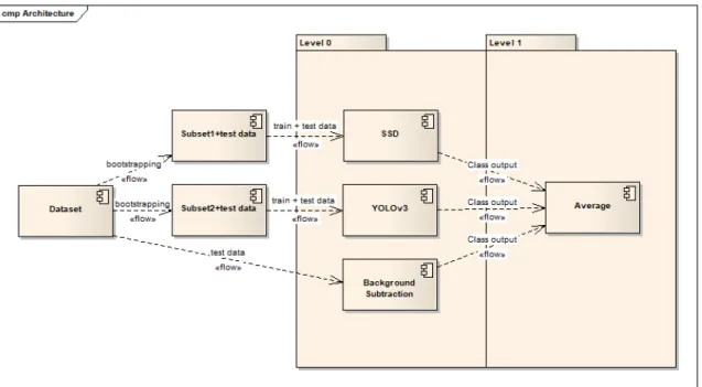
3.3.2 Proposed System Architecture

Figure 3.2, below, represents our ensemble pipeline and the possible combinations:

Figure 3.3: Architecture of the ensemble solution with majority voting as combination

We propose a Bagging strategy with the pasting small votes variation, since according to [Polikar, 2006] it is a good approach when available data is of limited size and also when there are unstable models to help ensure diversity (neural networks are unstable models). Although Boosting is also an ensemble methodology that can achieve good classification results, it is not suitable for our proposed solution since, as can be seen on the following paragraph, we are using computationally heavy learners(YOLO and SSD) and Boosting is based on weak learners that can be trained over and over.

The classification algorithms that compose the proposed ensemble are SSD, YOLO and Back-ground Subtraction. SSD performs well with vehicle datasets, as it is presented in figure 3 of [W. Liu, 2016], while being faster to train than the two-stage approaches like faster-RCNN that take a long time to train and it is already integrated in the current pipeline so it is important to have for comparison with the newer solution.

YOLOv3 the latest iteration of YOLO, has the quickest inference times of current classification algorithms as can be found in [J. Redmon, 2018] and for classification with mobility applications it is important to have the fastest algorithms possible. Finally background subtraction is a weak algorithm that was one of the first attempts of classifying vehicles and for comparison purposes it is interesting to have with the other two more recent methods.

3.3.2.1 SSD

The version existing in the original pipeline and chosen to be a part of the ensemble is SSD Incep-tion which is a SSD model architecture with an incepIncep-tion network. So we can only assume that the application behind the inception theory [Szegedy et al., 2015] with the SSD model. Normal SSD

has densely connected layers while SSD Inception has sparsely connected layers, while densely layers connect to every next layer, sparsely does not connect to all layers but instead connect to a concatenation layer.

Figure 3.4: Architecture of normal SSD taken from [W. Liu, 2016]

In Figure 3.4, above, there are fully connected convolutional layers. With inception those fully connected become sparsely connected with a filter concatenation at the end.

Figure 3.5: Diagram of the idea behind inception [Szegedy et al., 2015]

SSD was trained with 3 classes motorcycles, light vehicles and heavy vehicles. It uses 2 data augmentation options, random cropping and random horizontal flip. We mostly trained SSD for 50 000 iterations per dataset. Acceptance threshold for detection and classification was 50%.

3.3.2.2 YOLO

For the used datasets, YOLOv3 would require 1900MB of VRAM and the training time for all 3 datasets would not be within the thesis time frame, therefore we chose to perform the training with tiny YOLOv3 which has less convolutional layers therefore uses 400MB of VRAM.

Tiny YOLO is composed of 13 convolutional layers and 2 YOLO output layers, each of the first 6 convolutional layers is followed by a maxpooling operation of size 2. We trained yolo on 3 classes, so each of the convolutional layers before the YOLO layers has a filter of size 24 as presented in the guide for YOLO and in SSD’s paper [W. Liu, 2016] (classes + 5) ∗ 3. YOLO downsamples by a factor of 32 so every image size has to be a multiple of 32.

Table 3.1: Architecture of YOLO tiny based of [J. Redmon, 2018] Type Filters Size/Stride Output

Convolutional 16 3x3 256x256 Maxpool 2x2/2 128x128 Convolutional 32 3x3 128x128 Maxpool 2x2/2 64x64 Convolutional 64 3x3 64x64 Maxpool 2x2/2 32x32 Convolutional 128 3x3 32x32 Maxpool 2x2/2 16x16 Convolutional 256 3x3 16x16 Maxpool 2x2/2 8x8 Convolutional 512 3x3 8x8 Maxpool 2x2/2 4x4 Convolutional 256 1x1 4x4 Convolutional 512 3x3 4x4 Convolutional 1x1 4x4 AvgPool Global Connected 1000 Softmax

We trained YOLO with a learning rate of 0.0004 and batch size of 64. The acceptance thresh-old for detection and classification was 50%.

3.3.2.3 Background Subtraction

This classifier is the simplest and the fastest, it is based on MOG (mixture of gaussians)[T. Bouwmans, 2008].To the resulting foreground image we applied the algorithm for edge detection [Suzuki and Be, 1985].

Figure 3.6: Flow chart of the operations for extracting the background. Each of the background subractors are MOG background subractors

Finally we used dimension heuristics to remove contours that do not represent vehicles. For each camera a region for classification on each lane is selected. The region for each camera is a critical part of the method since class is given based on area threshold, everything above the threshold is a heavy and everything below is a light vehicle.

The next figure shows the region coded for the classification in the first dataset.

Figure 3.7: Regions chosen for background subtraction classification on dataset 1,area threshold is 1890 pixels

Figure 3.8: Regions chosen for background subtraction classification on dataset 2 The next figure shows the region chosen for the classification in dataset 3.

Figure 3.9: Regions chosen for background subtraction classification on dataset 3, area threshold is 60 000 pixels

Since background subtraction only classifies objects based on area and does not use any fea-tures then we associated a probability with each class. Light vehicles and motorcycles have 0.5 probability since the area of the contour boxes is not very different and this probability affects combination as we explain in the next subsection. Heavy vehicles have a higher probability of 0.7 since they have a more distinctive area.

3.3.2.4 Combination

For the combinational part, each dataset is divided into two parts, 70% of the vehicle samples are used for training while the remaining 30% are used for testing. The training part, is further divided into two halves that are fed into the two classifiers (SSD and YOLO).

The test set is the same for all the learners and will be used to serve as the data for combining the predictions of the different learners, in order to retrieve an evaluation of the single and combined predictions over the same data.

Background subtraction is implemented in a way that only classifies certain regions closer to the camera where we know the area threshold between the different classes of vehicles. Even though both learners, SSD and YOLO, output classification for the full image, doing the same on background subtraction would result in a complete randomness of predictions since the area of a vehicle box depends on how far of the camera it is.

It must be stated that Background subtraction is not a learning algorithm so it does not receive a dataset to train only the one to test.

Each algorithm is different and outputs classification differently but in order to compare all the algorithms a uniformization of output is required. To that end, for each frame or image of the test set, each model writes a predictions file <frame>-<model>.txt. Each line of the file is composed of <class> <probability> <x> <y> <width> <height> all the models output a file in that format at the end of the test phase. x, y, width, height are all aspect ratios and x and y are centroid coordinates, some of the models output the format in centroids and others in coordinates of the bounding box corners so for those we calculated the centroids.

To combine the outputs a python script was implemented, which goes frame by frame opening the output files of each model and compare each line to see which are similar since being similar means that they classify the same object. We find similarity by calculating the IOU(Intersect over Union) between the boxes which definition is shown next.

Figure 3.10: Definition of IOU, image taken from PyImageSearch an Image Search engines blog [Rosebrock, 2018]

Two methods for calculating the final prediction were implemented Max Voting also known as Majority Voting and Best Average . For Best Average if the similar lines have the same class

prediction then we sum probability, x, y, width and height then divide it by number of similar lines, the final classification is the one with higher probability.

Algorithm 1 Best Average

1: box . list that has the bounding box probability, centroid coordinates in aspect ratios, width and height

2: Zc . number of classifiers that predicted for this frame with class c 3: listAverages . list to store the averages for each class

4: sumc← ∑Z_n=1c boxn

5: listAverages.append(sumc/Zc) 6: return max(listAverages)

We also created a max voting combination method as a second option. Each classification algorithms has the same vote weight in the case that there is a tie in the number of votes then the tiebreaker is having the highest probability. A classifier votes towards a class for an object by predicting for it.

Algorithm 2 Max Voting also known as Majority Voting

1: dictionaryVotes. dictionary of votes per class ordered from the most voted to the least voted

2: dictionaryProb . dictionary of best(highest probability) per class list with outputed by classifier bounding box and associated probability

3: maxelem← dictionaryVotes.key(0)

4: i← 0

5: for i < dictionaryVotes.length do

6: elem← dictionaryVotes.key(i)

7: if dictionaryVotes.get(elem) == dictionaryVotes.get(maxelem) then

8: if dictionaryProb.get(elem) > dictionaryProb.get(maxelem) then

9: maxelem← elem

10: end if

11: end if

12: i← i + 1

13: end for

14: return maxelem, dictionaryProb.get(maxelem) . The Majority voted class is maxelem and the box associated is dictionaryProb.get(maxelem)

In the scenario that only one model has a prediction for a given object, then we used a threshold of 50% of class probability to trust the prediction, in order to reduce the situations of a single model introducing miss classifications.

For evaluating the methods we chose the average precision, F1 score and the hit rate, by hit rate we mean the percentage of annotations that the models and combination predicted correctly. We excluded the classification accuracy metric since there is a large class imbalance between heavy and light vehicles. This is even worse when there are motorcycles. The hit rate is the most useful one since it is the main comparison point between classifiers to evaluate if there are more or less vehicles being missed and the gain between the individual models and the combination.