Search for supersymmetry in events with b-quark jets and missing transverse energy in pp collisions at 7 TeV

EUROPEAN ORGANIZATION FOR NUCLEAR RESEARCH (CERN)

CERN-PH-EP/2012-240 2013/01/29

CMS-SUS-12-003

Search for supersymmetry in events with b-quark jets and

missing transverse energy in pp collisions at 7 TeV

The CMS Collaboration

∗

Abstract

Results are presented from a search for physics beyond the standard model based on events with large missing transverse energy, at least three jets, and at least one, two, or three b-quark jets. The study is performed using a sample of proton-proton collision data collected at√s =7 TeV with the CMS detector at the LHC in 2011. The integrated luminosity of the sample is 4.98 fb−1. The observed number of events is found to be consistent with the standard model expectation, which is evaluated using control samples in the data. The results are used to constrain cross sections for the production of supersymmetric particles decaying to b-quark-enriched final states in the context of simplified model spectra.

Submitted to Physical Review D

∗_{See Appendix A for the list of collaboration members}

1

1

Introduction

Many extensions of the standard model (SM) predict that events in high-energy proton-proton collisions can contain large missing transverse energy (E_Tmiss) and multiple, high-transverse mo-mentum (pT) jets. For example, in R-parity-conserving [1] models of supersymmetry (SUSY) [2],

SUSY particles are created in pairs. Each member of the pair initiates a decay chain that terminates with the lightest SUSY particle (LSP) and SM particles. If the LSP only interacts weakly, as in the case of a dark-matter candidate, it escapes detection, potentially yielding sig-nificant Emiss

T . Furthermore, in some scenarios [3], the SUSY partners of the bottom and top

quarks can be relatively light, leading to the enhanced production of events with bottom-quark jets (b jets). Events of this type, with b jets and large Emiss_T , represent a distinctive topological signature that is the subject of a search described in this paper.

We present a search for new physics (NP) in events with large Emiss_T , no isolated leptons, three or more high-pTjets, and at least one, two, or three b jets. The analysis is based on a sample of

proton-proton collision data collected at√s = 7 TeV with the Compact Muon Solenoid (CMS) detector at the CERN Large Hadron Collider (LHC) in 2011, corresponding to an integrated luminosity of 4.98 fb−1. Recent searches for NP in a similar final state are presented in Refs. [4– 8]. Our analysis is characterized by a strong reliance on techniques that use control samples in data to evaluate the SM background.

The principal sources of the SM background are events with top quarks, comprising tt pair and single-top-quark events, events with a W or Z boson accompanied by jets, and non-top multijet events produced purely through strong-interaction processes. We hereafter refer to this last class of events as “QCD” background. Diboson (WW, ZZ, or WZ) events represent a smaller source of background. For events with a W boson or a top quark, significant Emiss_T can arise if a W boson decays into a charged lepton and a neutrino. The neutrino provides a source of genuine Emiss

T . Similarly, significant EmissT can arise in events with a Z boson if the Z

boson decays to two neutrinos. For QCD background events, significant Emiss

T arises primarily

from the mismeasurement of jet pT. A smaller component of the QCD background arises from

events with semileptonic decays of b and c quarks.

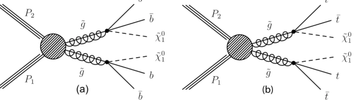
We interpret our results in the context of simplified model spectra (SMS) [9–12], which pro-vide a general framework to characterize NP signatures. They include only a few NP particles and focus on generic topologies. We consider the SMS scenarios denoted T1bbbb and T1tttt. Event diagrams are shown in Fig. 1. These two models are characterized by b-jet-enriched fi-nal states, large jet multiplicities, and large Emiss

T values, making our analysis sensitive to their

production. For convenience, we express SMS phenomenology using SUSY nomenclature. In T1bbbb (T1tttt), pair-produced gluinoseg each decay into two b-quark jets (t-quark jets) and the LSP, taken to be the lightest neutralinoχe

0_{. The LSP is assumed to escape detection, leading to}

significant Emiss_T . If the SUSY partner of the bottom quark (top quark) is much lighter than any other squark, with the gluino yet lighter, gluino decays are expected to be dominated by the three-body process shown in Fig. 1(a) [Fig. 1(b)].

As benchmark NP scenarios, we choose the T1bbbb and T1tttt models with gluino mass m

e g =

925 GeV and LSP mass mLSP=100 GeV, with normalization to the next-to-leading order (NLO)

plus next-to-leading-logarithm (NLL) cross section [13–17]. These two benchmark models lie near the boundary of our expected sensitivity.

In Sections 2-3 we describe the detector and event selection. Section 4 introduces the ∆ ˆφmin

variable, used in the evaluation of the QCD background. Our techniques to evaluate the SM background from control samples in data are presented in Section 5. In Section 6 we describe

our analysis framework, based on a likelihood method that simultaneously determines the SM background and tests the consistency of NP models with the data, taking into account possible NP contamination of control sample regions. The interpretation of our results is presented in Section 7. A summary of the analysis is given in Section 8.

P1 P2 ˜g ˜g ¯b b ˜χ0 1 ˜χ0 1 ¯b b (a) P1 P2 ˜g ˜g ¯t t ˜χ0 1 ˜χ0 1 ¯t t (b)

Figure 1: Event diagrams for the (a) T1bbbb and (b) T1tttt simplified models.

2

Detector and trigger

A detailed description of the CMS detector is given elsewhere [18]. The CMS coordinate sys-tem is defined with the origin at the center of the detector and the z axis along the direction of the counterclockwise beam. The transverse plane is perpendicular to the beam axis, with φ the azimuthal angle (measured in radians), θ the polar angle, and η = −ln[tan(θ/2)]the pseudo-rapidity. A superconducting solenoid provides an axial magnetic field of 3.8 T. Within the field volume are a silicon pixel and strip tracker, a crystal electromagnetic calorimeter, and a brass-scintillator hadron calorimeter. Muons are detected with gas-ionization chambers embedded in the steel flux-return yoke outside the solenoid. The tracker covers the region|η| <2.5 and the calorimeters|η| < 3.0. The region 3< |η| <5 is instrumented with a forward calorimeter. The near-hermeticity of the detector permits accurate measurements of energy balance in the transverse plane.

The principal trigger used for the analysis selects events based on the quantities HTand H_Tmiss,

where HT is the scalar sum of the transverse energy of jets and HTmissthe modulus of the

cor-responding vector sum. Due to increasing beam collision rates, trigger conditions varied over the period of data collection. The most stringent trigger requirements were HT >350 GeV and

H_Tmiss > 110 GeV. The efficiency of the HT component for the final event selection is measured

from data to be 86% (99%) for HTvalues of 400 GeV (500 GeV). The efficiency of the H_Tmiss

com-ponent is 98% for Emiss

T > 250 GeV. Appropriate corrections are applied to account for trigger

inefficiencies and uncertainties in the various control and search regions of the analysis.

3

Event selection

Physics objects are defined using the particle flow (PF) method [19], which is used to recon-struct and identify charged and neutral hadrons, electrons (with associated bremsstrahlung photons), muons, tau leptons, and photons, using an optimized combination of information from CMS subdetectors. The PF objects serve as input for jet reconstruction, based on the anti-kT algorithm [20] with distance parameter 0.5. Jet corrections [21] are applied to account for

residual effects of non-uniform detector response in both pT and η. The missing transverse

energy Emiss_T is defined as the modulus of the vector sum of the transverse momenta of all PF objects. The Emiss_T vector is the negative of the same vector sum.

3

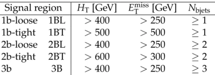
Table 1: The definition of the signal (SIG) regions. The minimum requirements on HT, EmissT ,

and the number of tagged b jets Nbjets are given. The designations 1b, 2b, and 3b refer to the

minimum Nbjets value, while “loose” and “tight” refer to less restrictive and more restrictive

selection requirements, respectively, for HTand ETmiss.

Signal region HT[GeV] Emiss_T [GeV] Nbjets

1b-loose 1BL >400 >250 ≥1

1b-tight 1BT >500 >500 ≥1

2b-loose 2BL >400 >250 ≥2

2b-tight 2BT >600 >300 ≥2

3b 3B >400 >250 ≥3

The basic event selection criteria are as follows:

• at least one well-defined primary event vertex [22]; • at least three jets with pT >50 GeV and|η| <2.4;

• a lepton veto defined by requiring that there be no identified, isolated electron or muon candidate [23, 24] with pT > 10 GeV; electron candidates are restricted to

|η| <2.5 and muon candidates to|η| <2.4;

• ∆ ˆφ_min >4.0, where the∆ ˆφminvariable is described in Section 4.

Electrons and muons are considered isolated if the scalar sum of the transverse momenta of charged hadrons, photons, and neutral hadrons surrounding the lepton within a cone of radius p

(∆η)2_{+ (∆φ)}2 _{=0.3, divided by the lepton p}

Tvalue itself, is less than 0.20 for electrons and

0.15 for muons.

To identify b jets, we use the combined-secondary-vertex algorithm at the medium working point [25]. This algorithm combines information about secondary vertices, track impact pa-rameters, and jet kinematics, to separate b jets from light-flavored-quark, charm-quark, and gluon jets. To increase sensitivity to NP scenarios, which often predict soft b jets, we use all tagged b jets with pT >30 GeV. The nominal b-jet-tagging efficiency is about 75% for jets with

a pT value of 100 GeV, as determined from a sample of b-jet-enriched dijet events [25] (for b

jets with pT ≈ 30 GeV, this efficiency is about 60%). The corresponding misidentification rate

is about 1.0%. We correct the simulated efficiencies for b-jet tagging and misidentification to match the efficiencies measured with control samples in the data. The b-tagging correction factor depends slightly on the jet pT and has a typical value of 0.95. The uncertainty on this

correction factor varies from 0.03 to 0.07 for b jets with pT from 30 to 670 GeV, and is taken to

be 0.13 for b jets with pT>670 GeV.

We define five signal regions, which partially overlap, to enhance sensitivity in different kine-matic regimes. The five regions correspond to different minimum requirements on HT, Emiss_T ,

and the number of b jets. HT is calculated using jets with pT >50 GeV and|η| <2.4. The five

regions, denoted 1BL, 1BT, 2BL, 2BT, and 3B, are specified in Table 1 and were chosen without considering the data to avoid possible bias. The regions are selected based on expected signal and background event yields in simulation, to provide maximal sensitivity for discovery of the NP scenarios considered in this paper or, in the case of non-discovery, to best set limits on their parameters. Throughout this paper, we use the generic designation “SIG” to refer to any or all of these five signal regions.

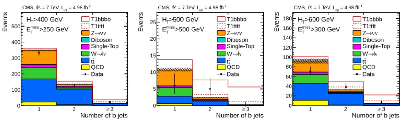
The distributions of the number of tagged b jets for the 1BL, 1BT, and 2BT samples (i.e., for the three different sets of selection criteria on HT and ETmiss), except without the requirement

Number of b jets 1 2 ≥ 3 Events 0 100 200 300 400 500 -1 = 4.98 fb int = 7 TeV, L s CMS, >400 GeV T H >250 GeV miss T E T1bbbb T1tttt ν ν → Z Diboson Single-Top ν l → W t t QCD Data Number of b jets 1 2 ≥ 3 Events 0 5 10 15 20 25 -1 = 4.98 fb int = 7 TeV, L s CMS, >500 GeV T H >500 GeV miss T E T1bbbb T1tttt ν ν → Z Diboson Single-Top ν l → W t t QCD Data Number of b jets 1 2 ≥ 3 Events 0 20 40 60 80 100 120 140 160 180 -1 = 4.98 fb int = 7 TeV, L s CMS, >600 GeV T H >300 GeV miss T E T1bbbb T1tttt ν ν → Z Diboson Single-Top ν l → W t t QCD Data

Figure 2: The distributions of the number of tagged b jets for event samples selected with the (a) 1BL, (b) 1BT, and (c) 2BT requirements, except for the requirement on the number of b jets. The hatched bands show the statistical uncertainty on the total SM background prediction from simulation. The open histograms show the expectations for the T1bbbb (solid line) and T1tttt (dashed line) NP models, both with m_eg = 925 GeV, mLSP = 100 GeV, and normalization to

NLO+NLL.

Monte Carlo (MC) simulations of SM processes. Results from the benchmark T1bbbb and T1tttt NP models mentioned in the Introduction are also shown. The simulated tt, W+jets, and Z+jets events are produced at the parton level with the MADGRAPH5.1.1.0 [26] event gen-erator. Single-top-quark events are generated with thePOWHEG301 [27] program. ThePYTHIA

6.4.22 program [28] is used to produce diboson and QCD events. For all simulated samples,

PYTHIA6.4 is used to describe parton showering and hadronization. All samples are generated using the CTEQ6 [29] parton distribution functions. The description of the detector response is implemented using the GEANT4 [30] program. The tt sample is normalized to the measured

cross section [31]. The other simulated samples are normalized using the most accurate cross section calculations currently available, which is generally NLO. The jet energy resolution in the simulation is corrected to account for a small discrepancy with respect to data [21]. In ad-dition, the simulated samples are reweighted to describe the probability distribution observed in data for overlapping pp collisions within a bunch crossing (“pileup”).

[GeV] miss T E 200 250 300 350 400 450 500 Events 0 20 40 60 80 100 120 140 160 180 200 220 T1bbbb T1tttt ν ν → Z Diboson Single-Top ν l → W tt QCD Data -1 = 4.98 fb int = 7 TeV, L s CMS, 1BL selection (a) [GeV] miss T E 200 250 300 350 400 450 500 Events 0 10 20 30 40 50 60 70 80 90 _T1bbbb T1tttt ν ν → Z Diboson Single-Top ν l → W tt QCD Data -1 = 4.98 fb int = 7 TeV, L s CMS, 2BT selection (b) [GeV] miss T E 200 250 300 350 400 450 500 Events 0 5 10 15 20 25 30 T1bbbb T1tttt ν ν → Z Diboson Single-Top ν l → W tt QCD Data -1 = 4.98 fb int = 7 TeV, L s CMS, 3B selection (c)

Figure 3: The distributions of Emiss_T for event samples selected with the (a) 1BL, (b) 2BT, and (c) 3B requirements, except for the requirement on Emiss

T . The simulated spectra are normalized

as in Fig. 2. The hatched bands show the statistical uncertainty on the total SM background prediction from simulation. The rightmost bin in all plots includes event overflow. The open histograms show the expectations for the T1bbbb (solid line) and T1tttt (dashed line) NP mod-els, both with m_eg=925 GeV, mLSP=100 GeV, and normalization to NLO+NLL.

5

Table 2: The number of data events and corresponding predictions from MC simulation for the signal regions, with normalization to 4.98 fb−1. The uncertainties on the simulated results are statistical. 1BL 1BT 2BL 2BT 3B Data 478 11 146 45 22 Total SM MC 496±7 13.3±0.6 148±2 36.8±0.9 15.0±0.2 tt 257±2 3.6±0.2 111±1 26.7±0.4 12.6±0.2 Single-top quark 26.0±1.0 0.8±0.2 9.1±0.5 2.7±0.3 0.88±0.09 W+jets 80.0±1.0 2.8±0.2 7.7±0.3 2.2±0.2 0.38±0.05 Z→νν 104±2 5.3±0.4 13.8±0.7 3.5±0.3 0.80±0.10 Diboson 1.8±0.1 0.10±0.02 0.27±0.04 0.05±0.02 0.02±0.01 QCD 28.0±6.0 0.70±0.20 6.0±1.0 1.7±0.6 0.29±0.07

jets, the E_Tmissdistributions of events in the 1BL, 2BT, and 3B samples are shown in Fig. 3. The numbers of events in the different signal regions are listed in Table 2 for data and simulation. The simulated results are for guidance only and are not used in the analysis.

4

The

∆ ˆφ

_min

variable

Figure 4: Illustration of variables used to calculate∆ ˆφminfor the case of an event with exactly

three jets with pT >30 GeV. The light-shaded (light gray) solid arrows show the true pTvalues

of the three jets i, j, and k. The dark-shaded (black) solid arrows show the reconstructed jet pT

values. The angles of jets j and k with respect to the direction opposite to jet i are denoted αj

and αk. The EmissT for the event is shown by the dotted (red) arrow. The component of EmissT

perpendicular to jet i, denoted Ti, is shown by the dotted (red) line. σTi is the uncertainty on Ti.

∆φi is the angle between Emiss_T and jet i.

Our method to evaluate the QCD background is based on the ∆ ˆφmin variable. This method

presumes that most E_Tmissin a QCD event arises from the pTmismeasurement of a single jet.

The ∆ ˆφmin variable is a modified version of the commonly used quantity∆φmin ≡ min(∆φi)

(i = 1, 2, 3), the minimum azimuthal opening angle between the Emiss_T vector and each of the three highest-pTjets in an event. Misreconstruction of a jet primarily affects the modulus of its

transverse momentum but not its direction. Thus QCD background events are characterized by small values of ∆φmin. The ∆φmin variable is strongly correlated with Emiss_T , as discussed

below. This correlation undermines its utility for the evaluation of the QCD background from data. To reduce this correlation, we divide the∆φiby their estimated resolutions σ∆φ,ito obtain

The resolution σ_∆φ,i for jet i is evaluated by considering the pT resolution σpT of the other jets

in the event. The uncertainty σTi on the component of the E

miss

T vector perpendicular to jet i

is found using σ_T2_i ≡ _∑n(σpT,nsin αn)

2_{, where the sum is over all other jets in the event with}

pT >30 GeV and αnis the angle between jet n and the direction opposite jet i. The situation is

depicted in Fig. 4 for an event with exactly three jets with pT > 30 GeV. Our estimate of the

∆φ resolution is σ_∆φ,i = arctan(σTi/ETmiss). [Note: arcsin(σTi/EmissT )is technically more correct

in this expression; we use arctan(σTi/E

miss

T ) because it is computationally more robust while

being equivalent for the small angles of interest here.] For the jet pTresolution, it suffices to use

the simple linear parametrization σpT =0.10 pT[21].

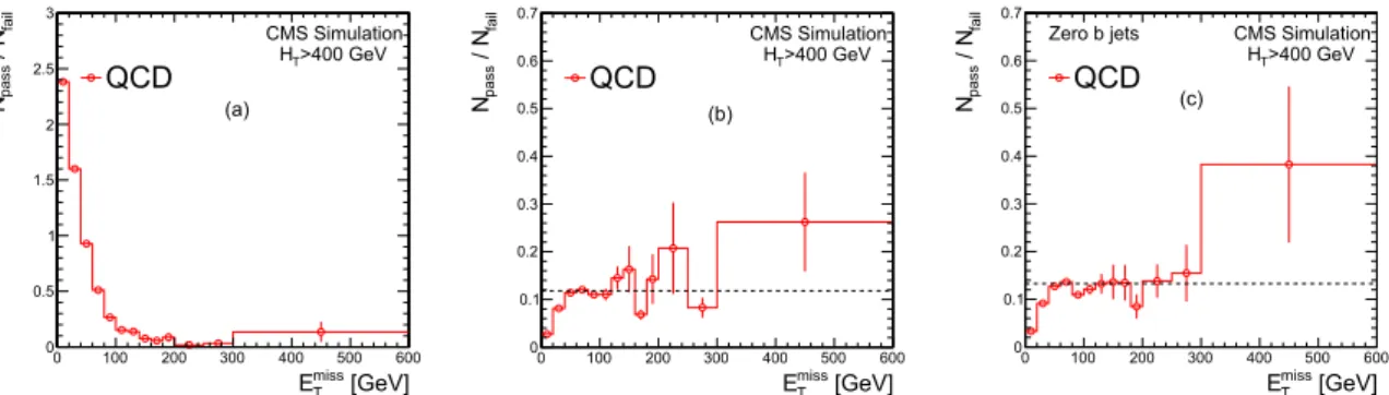
Figure 5(a) shows the ratio of the number of events with ∆φmin > 0.3 to the number with

∆φmin < 0.3 as a function of Emiss_T , for a simulated QCD sample selected with the 1BL

require-ments except for those on ∆ ˆφmin and EmissT (∆φmin > 0.3 or a similar criterion is commonly

used to reject QCD background, see, e.g., Refs. [5–8]). The strong correlation between ∆φmin

and E_Tmiss is evident. The corresponding result based on∆ ˆφmin is shown in Fig. 5(b). For the

latter figure we choose ∆ ˆφmin = 4.0 in place of∆φmin = 0.3, which yields a similar selection

efficiency. For values of Emiss

T greater than about 30 GeV, the distribution based on∆ ˆφmin is

seen to be far less dependent on Emiss

T than that based on∆φmin. Figure 5(c) shows the result

corresponding to Fig. 5(b) for events with zero tagged b jets. Comparing Figs. 5(b) and (c), it is seen that the ratio N(∆ ˆφmin≥ 4.0)/N(∆ ˆφmin <4.0)has an approximately constant value of

about 0.13 (for Emiss_T >30 GeV) irrespective of the number of b jets.

[GeV] miss T E 0 100 200 300 400 500 600 fail / N pass N 0 0.5 1 1.5 2 2.5 3 CMS Simulation QCD HT>400 GeV (a) [GeV] miss T E 0 100 200 300 400 500 600 fail / N pass N 0 0.1 0.2 0.3 0.4 0.5 0.6 0.7 CMS Simulation QCD HT>400 GeV (b) [GeV] miss T E 0 100 200 300 400 500 600 fail / N pass N 0 0.1 0.2 0.3 0.4 0.5 0.6 0.7 CMS Simulation QCD HT>400 GeV Zero b jets (c)

Figure 5: QCD-simulation results: (a) the ratio of the number of events that pass the criterion ∆φmin ≥0.3 (Npass) to the number that fail (Nfail) as a function of EmissT , for events selected with

the 1BL requirements except for those on ∆ ˆφmin and Emiss_T ; (b) The analogous ratio of events

with∆ ˆφmin ≥4.0 to those with∆ ˆφmin <4.0; and (c) the same as (b) for events with zero b jets.

The QCD-background estimate is based on the relative flatness of the distributions in (b) and (c) for E_Tmiss >_{∼30 GeV, as illustrated schematically by the dashed lines.}

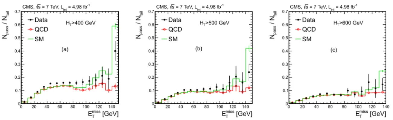
The measured results for N(∆ ˆφ_min ≥ 4.0)/N(∆ ˆφ_min < 4.0) with zero b jets, for events with HT > 400 GeV, 500 GeV, and 600 GeV, are shown in Fig. 6. By requiring that there not be a

b jet, we reduce the contribution of top-quark events, which is helpful for the evaluation of QCD background (Section 5.1). The data in Fig. 6 are collected with a pre-scaled HT trigger,

allowing events to be selected at low E_Tmisswithout a trigger bias. The data in Fig. 6(a) are seen to somewhat exceed the simulated predictions. The trend is visible in Fig. 6(b) to a lesser extent. This modest discrepancy arises because the ∆ ˆφmin distribution is narrower in the simulation

than in data. Since our method to evaluate the QCD background is based on the measured distribution, this feature of the simulation does not affect our analysis. The data in Fig. 6 are seen to exhibit the general behavior expected from the simulation. The region below around 100 GeV is seen to be dominated by the QCD background.

7 [GeV] miss T E 0 20 40 60 80 100 120 140 fail / N pass N 0 0.1 0.2 0.3 0.4 0.5 0.6 0.7 -1 = 4.98 fb int = 7 TeV, L s CMS, Data QCD SM >400 GeV T H (a) [GeV] miss T E 0 20 40 60 80 100 120 140 fail / N pass N 0 0.1 0.2 0.3 0.4 0.5 0.6 0.7 -1 = 4.98 fb int = 7 TeV, L s CMS, Data QCD SM >500 GeV T H (b) [GeV] miss T E 0 20 40 60 80 100 120 140 fail / N pass N 0 0.1 0.2 0.3 0.4 0.5 0.6 0.7 -1 = 4.98 fb int = 7 TeV, L s CMS, Data QCD SM >600 GeV T H (c)

Figure 6: The ratio N(∆ ˆφ_min ≥ 4.0)/N(∆ ˆφ_min < 4.0), denoted Npass/Nfail, as a function of

Emiss

T for the zero-b-jet sample, for events selected with the basic event selection criteria of the

analysis except for the requirements on E_Tmissand the number of b jets. The results are shown for (a) HT > 400 GeV, (b) HT > 500 GeV, and (c) HT > 600 GeV. The histograms show simulated

predictions for the QCD and total SM background.

5

Background evaluation

In this section we describe our methods to evaluate the SM background from control samples in data. Each of the three main backgrounds – from QCD, Z+jets, and top-quark and W+jets events (where “top quark” includes both tt and single-top-quark events) – is evaluated sepa-rately. We group top quark and W+jets events together because they have a similar experimen-tal signature. Note that our final results for the toexperimen-tal SM background are derived from a global likelihood procedure that incorporates our background evaluation procedures into a single fit, and that also accounts for possible NP contributions to the control regions in a consistent man-ner. The global likelihood procedure is described in Section 6.

QCD background is evaluated using the ∆ ˆφmin variable. Background from Z+jets events is

evaluated by scaling the measured rates of Z → `+<sub>`</sub>− _{(` =e or µ) events. To estimate the}

top-quark and W+jet background, we employ two complementary techniques. One, which we call the nominal method, is simple and almost entirely data based, while the other, which we call the Emiss

T -reweighting method, combines results based on data with information from

simulation to examine individual sources of top-quark and W+jets background in detail.

5.1 QCD background

The low level of correlation between ∆ ˆφmin and E_Tmiss allows us to employ a simple method

to evaluate the QCD background from data. As discussed in Section 4, the ratio N(∆ ˆφ_min ≥ 4.0)/N(∆ ˆφ_min < 4.0)is approximately independent of E_Tmiss, and also of the number of b jets, for QCD events. Furthermore, the E_Tmissdistribution below 100 GeV is expected to be dominated by QCD events, especially for events with zero b jets (Fig. 6). We therefore measure N(∆ ˆφ_min ≥ 4.0)/N(∆ ˆφ_min < 4.0) in a low Emiss

T region of the zero-b-jet sample and assume this equals

N(∆ ˆφ_min ≥ 4.0)/ N(∆ ˆφ_min < 4.0)for QCD events at all Emiss

T values, also for samples with b

jets such as our signal samples.

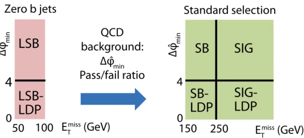
To perform this measurement, we divide the data into sideband and signal regions in the∆ ˆφmin

-E_Tmiss plane, as illustrated schematically in Fig. 7. We use the low-E_Tmiss interval defined by 50< E_Tmiss<100 GeV and∆ ˆφmin>4.0. We call this interval the low sideband (LSB) region. We

also define low∆ ˆφmin (LDP) intervals∆ ˆφmin < 4.0. We do this not only for the 50 < E_Tmiss <

100 GeV region, but also for the signal regions (SIG) and for a sideband (SB) region defined by 150< Emiss

T <250 GeV. We denote these regions LSB-LDP, SIG-LDP, and SB-LDP, respectively.

QCD

background:

∆φˆ

_min

Pass/fail ratio

E

_Tmiss

_(GeV)

SB

SIG

SB-LDP

SIG-

LDP

LSB-LDP

LSB

∆φ

ˆ

min

∆φ

ˆ

min

4

50 100

0

150 250

E

_Tmiss

_(GeV)

4

0

Zero b jets

Standard selection

Figure 7: Schematic diagram illustrating the regions used to evaluate the QCD background. The low sideband (LSB) and low sideband-low ∆ ˆφmin(LSB-LDP) regions correspond to 50 <

E_Tmiss < 100 GeV. The sideband (SB) and sideband-low ∆ ˆφmin (SB-LDP) regions correspond

to 150 < E_Tmiss < 250 GeV. The signal (SIG) and signal-low ∆ ˆφmin (SIG-LDP) regions have

E_Tmiss ranges corresponding to those in Table 1. The designation “SIG” generically refers to any of the signal regions in this table. The SIG and SIG-LDP regions shown in the diagram explicitly depict the loose kinematic signal regions 1BL, 2BL, and 3B, which require Emiss

T >

250 GeV, but implicitly include the tight kinematic signal regions 1BT and 2BT, which require E_Tmiss > 500 GeV and 300 GeV, respectively. For each choice of signal region, the condition on HT specified in Table 1 for that region is applied to all six panels of the diagram, while the

condition on the number of b jets is applied to the four panels denoted “Standard selection.” All regions with the low∆ ˆφmin (LDP) designation require 0.0 < ∆ ˆφmin < 4.0, while the other

5.1 QCD background 9

Table 3: The relative systematic uncertainties (%) for the QCD background estimate in the signal regions. Because the 1BT QCD background estimate is zero (Section 5.5), we do not present results for 1BT in this table.

1BL 2BL 2BT 3B

MC subtraction 23 43 44 24

MC closure 37 41 150 45

LSB reweighting 7.9 7.9 9.8 7.9

Total 44 60 160 52

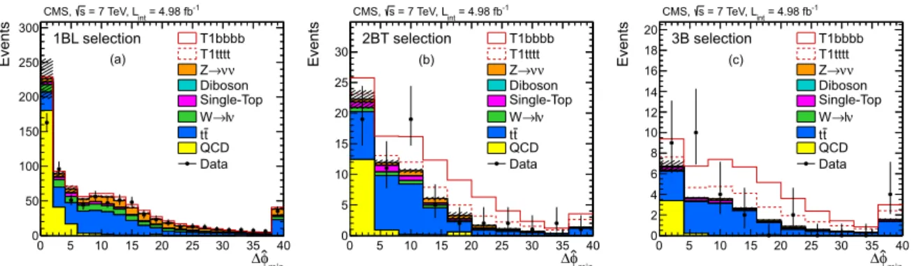
largely consist of QCD events, as illustrated for the 1BL, 2BT, and 3B SIG-LDP regions in Fig. 8 (according to simulation, QCD events comprise between 73% and 85% of the events in the SB-LDP region, depending on the SIG selection; the corresponding results for for the SIG-SB-LDP region lie between 50% and 70%). For higher values of Emiss_T , contributions to the SB-LDP and SIG-LDP regions from events with a top quark or a W or Z boson become more important. This contamination is subtracted using simulation.

min φ ∆ 0 5 10 15 20 25 30 35 40 Events 0 50 100 150 200 250 300 T1bbbb T1tttt ν ν → Z Diboson Single-Top ν l → W tt QCD Data -1 = 4.98 fb int = 7 TeV, L s CMS, 1BL selection (a) min φ ∆ 0 5 10 15 20 25 30 35 40 Events 0 5 10 15 20 25 30 T1bbbb_T1tttt ν ν → Z Diboson Single-Top ν l → W tt QCD Data -1 = 4.98 fb int = 7 TeV, L s CMS, 2BT selection (b) min φ ∆ 0 5 10 15 20 25 30 35 40 Events 0 2 4 6 8 10 12 14 16 18 20 _T1bbbb T1tttt ν ν → Z Diboson Single-Top ν l → W tt QCD Data -1 = 4.98 fb int = 7 TeV, L s CMS, 3B selection (c)

Figure 8: The distributions of∆ ˆφminin data and simulation for events selected with the (a) 1BL,

(b) 2BT, and (c) 3B requirements, except for the requirement on∆ ˆφmin. The simulated spectra

are normalized as in Fig. 2. The hatched bands show the statistical uncertainty on the total SM prediction from simulation. The open histograms show the expectations for the T1bbbb (solid line) and T1tttt (dashed line) NP models, both with m_eg=925 GeV, mLSP=100 GeV, and

normalization to NLO+NLL. The SIG-LDP regions correspond to∆ ˆφmin < 4.0 and the signal

(SIG) regions to∆ ˆφmin >4.0.

Applying corrections for the non-QCD components of the SIG-LDP and SB-LDP regions, our estimates of the QCD yields in the SIG and SB regions are therefore:

N_SIGQCD = NLSB

NLSB−LDP

× (N_SIG−LDP−NSIGtop,MC−LDP−N

W&Z,MC SIG−LDP), (1) N_SBQCD = NLSB NLSB−LDP × (NSB−LDP−N_SBtop,MC−LDP−N W&Z,MC SB−LDP ), (2)

where the LSB and LSB-LDP results are derived from the zero-b-jet, pre-scaled HTtrigger

sam-ple mentioned in Section 4. The result for N_SBQCDis used in Section 5.3. The ratio NLSB/NLSB−LDP

is found to depend on the number of primary vertices (PV) in the event and thus on the LHC instantaneous luminosity. Before evaluating Eqs. (1) and (2), we therefore reweight the events in the pre-scaled sample to have the same PV distribution as the standard sample.

Systematic uncertainties are summarized in Table 3. The systematic uncertainty associated with the subtraction of events with either a top quark or a W or Z boson from the SIG-LDP and

SB-LDP regions is determined by varying the subtracted values by their uncertainties, evalu-ated as described in Section 7. The systematic uncertainty associevalu-ated with the assumption that E_Tmissand∆ ˆφminare uncorrelated is evaluated with an MC closure test, namely by determining

the ability of the method to predict the correct yield using simulated samples. We compute (Ntrue−Npred)/Npred, where Npredis the predicted number of QCD events in the signal region,

estimated by applying the above procedure to simulated samples treated as data, and Ntrue is

the true number. We assign the result, added in quadrature with its statistical uncertainty, as a symmetric systematic uncertainty. This uncertainty is dominated by statistical uncertainties for Ntrue. The closure test is performed both for the standard simulated samples and for simulated

samples that are reweighted to account for discrepancies in the jet multiplicity distributions between data and simulation; we take the larger closure discrepancy as the uncertainty. A third systematic uncertainty is evaluated by taking±100% of the shift in the result caused by the PV reweighting of NLSB/NLSB−LDP. The systematic uncertainty associated with the trigger

efficiency is found to be negligible.

As a cross-check, we vary the definition of the LSB by raising and lowering its lower edge by 10 GeV, which alters the number of events in the LSB by more than a factor of two in each case. The observed change in the QCD background estimate is negligible.

5.2 Z+jets background

Events with a Z boson and one or more b jets present an irreducible background when the Z decays to two neutrinos. We evaluate this background by reconstructing Z → `+<sub>`</sub>− _events

(` =e or µ) and removing the`+_{and`</sub>−<sub>. Fits are performed to determine the Z→ `}+_`−_yields,

which are then corrected for background and efficiency. The efficiency is e = A ·etrig·e2_{`reco</sub>· e2<sub>`sel}, where the geometrical acceptanceAis determined from simulation while the trigger etrig,

lepton reconstruction e`reco, and lepton selection e`sel efficiencies are determined from data.

The corrected Z → `+<sub>`</sub>− _{yields are used to estimate the Z→}

ννbackground through scaling by the ratio of branching fractions, BR(Z → νν)/BR(Z → `+`−) = 5.95±0.02 [32], after accounting for the larger acceptance of Z→ννevents.

The Z → `+<sub>`</sub>− _{yields are small or zero in the signal regions. To increase these yields, we}

select events with the signal-sample requirements except with a significantly looser b-tagging definition. A scale factor derived from a control sample in data is then applied to estimate the number of Z→ `+<sub>`</sub>−_{events in the signal regions. The control sample is defined with the same}

loosened b-tagging definition, but without requiring the presence of a Z boson, and also by reversing the∆ ˆφmin requirement, i.e., we require∆ ˆφmin < 4.0, which yields a control sample

with a b-jet content similar to that in the Z → `+<sub>`</sub>− _{and Z →}

ννevents. All other selection criteria are the same as for the corresponding signal sample. The scale factors are given by the fraction of events in the control sample that passes the nominal b-tagging requirements. The scale factors have values around 0.30, 0.07, and 0.01 for the samples with≥ 1, ≥ 2, and ≥ 3 b jets, respectively. We verify that the output of the b-tagging algorithm is independent of the presence of a Z.

We validate our method with a consistency test, applying the above procedure to data samples with loosened restrictions on HT and Emiss_T . We find the number of predicted and observed

Z→ `+<sub>`</sub>−_{events to be in close agreement.}

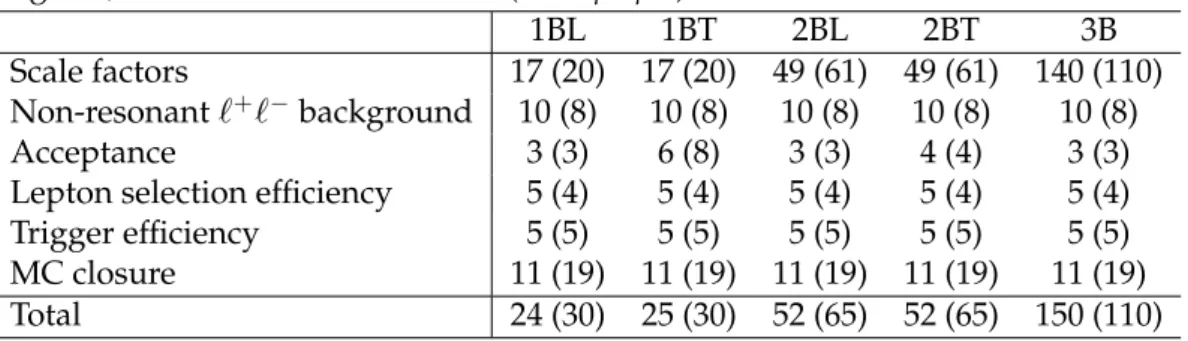
Systematic uncertainties are summarized in Table 4. We evaluate a systematic uncertainty on the scale factors by loosening and tightening the b-tagging criterion of the control sample and taking half the difference between the two results as an uncertainty. The size of the control sample changes by about±30% in these variations. In addition, we use ∆ ˆφmin > 4.0 rather

5.3 Top-quark andW+jets background (nominal) 11

Table 4: The relative systematic uncertainties (%) for the Z → ννbackground estimate in the signal regions, determined for Z→e+e−(Z→µ+µ−) events.

1BL 1BT 2BL 2BT 3B

Scale factors 17 (20) 17 (20) 49 (61) 49 (61) 140 (110)

Non-resonant`+`−background 10 (8) 10 (8) 10 (8) 10 (8) 10 (8)

Acceptance 3 (3) 6 (8) 3 (3) 4 (4) 3 (3)

Lepton selection efficiency 5 (4) 5 (4) 5 (4) 5 (4) 5 (4)

Trigger efficiency 5 (5) 5 (5) 5 (5) 5 (5) 5 (5)

MC closure 11 (19) 11 (19) 11 (19) 11 (19) 11 (19)

Total 24 (30) 25 (30) 52 (65) 52 (65) 150 (110)

than∆ ˆφmin < 4.0 to define the control sample and calculate the difference with respect to the

nominal results. Finally, we evaluate the percentage difference between the number of pre-dicted and observed events found with the consistency test described above. The three terms are added in quadrature to define the systematic uncertainty of the scale factors. We evaluate a systematic uncertainty associated with the non-resonant`+<sub>`</sub>−_{background to Z→ `</sub>+<sub>`}−_events

by comparing the fraction of fitted events in the Z → `+<sub>`</sub>− _{peak from the nominal fit with}

those found using either a loosened HT or a loosened EmissT restriction. The RMS of the three

results is added in quadrature with the statistical uncertainty from the nominal fit to define the systematic uncertainty. The 1BL selection is used to determine this uncertainty for all signal regions. A systematic uncertainty for the acceptance is defined by recalculating the acceptance after varying the pT and η ranges of the`+and`−. The largest difference with respect to the

nominal result is added in quadrature with the statistical uncertainty of the acceptance. A sys-tematic uncertainty is defined for the lepton selection efficiency, and analogously for the trigger efficiency, by recalculating the respective efficiency after varying the requirements on HT, Emiss_T ,

∆ ˆφmin, the number of jets, and the number of b jets (the number of jets is found using all jets

with pT > 50 GeV and|η| < 2.4). We also use alternative signal and background shapes in the fits used to extract the Z → `+<sub>`</sub>−_{event yields. The maximum variations from each case}

are added in quadrature with the statistical uncertainty from the nominal method to define the systematic uncertainties. Finally, we evaluate a systematic uncertainty based on an MC closure test in the manner described in Section 5.1. We use the SB region to determine this uncertainty. An analogous procedure to that described above is used to evaluate the number of Z → νν events NZ→νν

SB in the SB regions (150< EmissT < 250 GeV), along with the corresponding

uncer-tainty.

5.3 Top-quark and W+jets background (nominal)

For most signal regions, tt events are expected to be the dominant background (Table 2). Back-grounds from single-top-quark and W+jets events are expected to be smaller but to have a similar signature. Almost all top-quark and W+jets background in our analysis arises either because a W boson decays leptonically to an e or a µ, with the e or µ unidentified, not isolated, or outside the acceptance of the analysis, or because a W boson decays to a hadronically de-caying τ lepton. We find empirically, through studies with simulation, that the shape of the E_Tmissdistribution is similar for all top-quark and W+jets background categories that enter the signal (Table 1) or sideband (150 < E_Tmiss < 250 GeV) regions, regardless of whether the W boson decays to e, µ, or τ, or whether a τ lepton decays hadronically or leptonically: the decay of the W boson in W+jets events generates an E_Tmissspectrum (from the neutrino) that is similar to the Emiss_T spectrum generated by the W boson produced directly in the decay of a top quark in top quark events. Additional, softer neutrinos in events with a τ lepton do not much alter

this spectrum. We also find that this shape is well-modeled by the Emiss_T distribution of a single-lepton (SL) control sample formed by inverting the single-lepton veto, i.e., by requiring that exactly one e or one µ be present using the lepton identification criteria of Section 3, in a sample whose selection is otherwise the same as the corresponding signal sample, except to reduce the poten-tial contribution of NP to the SL samples, we impose an additional restriction MT < 100 GeV

on the SL samples (only), where MT is the transverse W-boson mass formed from the charged

lepton and E_Tmiss momentum vectors. As an illustration, Fig. 9 shows a comparison based on simulation of the E_Tmissdistributions in the signal and SL samples, for events selected with the 1BL, 2BT, and 3B criteria.

The Emiss_T distributions of events in the SL samples with the 1BL, 2BT, and 3B requirements are shown in Fig. 10. The distributions are seen to be overwhelmingly composed of tt events (for example, according to simulation, top and W+jets events comprise over 98% of the events in the SB-SL samples for all SIG selections). The expected contributions of the benchmark T1bbbb NP scenario are found to be negligible, while those of the benchmark T1tttt scenario are seen to be small in Fig. 10 compared to Fig. 3.

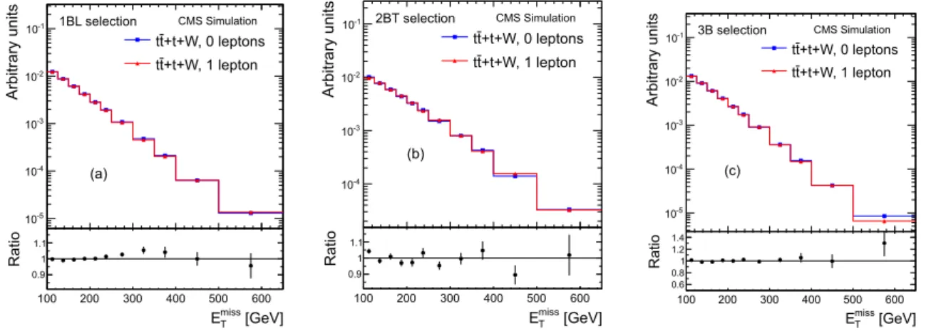
[GeV] miss T E 100 200 300 400 500 600 Arbitrary units -5 10 -4 10 -3 10 -2 10 -1 10 1BL selection CMS Simulation +t+W, 0 leptons tt +t+W, 1 lepton tt [GeV] miss T E 100 200 300 400 500 600 Ratio 0.9 1 1.1 (a) [GeV] miss T E 100 200 300 400 500 600 Arbitrary units -4 10 -3 10 -2 10 -1 10 2BT selection CMS Simulation +t+W, 0 leptons tt +t+W, 1 lepton tt [GeV] miss T E 100 200 300 400 500 600 Ratio 0.9 1 1.1 (b) [GeV] miss T E 100 200 300 400 500 600 Arbitrary units -5 10 -4 10 -3 10 -2 10 -1 10 3B selection CMS Simulation +t+W, 0 leptons tt +t+W, 1 lepton tt [GeV] miss T E 100 200 300 400 500 600 Ratio 0.6 0.81 1.2 1.4 (c)

Figure 9: The distributions of Emiss_T in simulated events selected with the (a) 1BL, (b) 2BT, and (c) 3B requirements, except for the requirement on Emiss_T . The square (triangle) symbols show the results for signal (single-lepton SL control) sample events. The small plots below the main figures show the ratio of the signal to SL sample curves. The event samples include tt, W+jet, and single-top-quark events.

Based on these observations, we implement a template method in which the shape of the Emiss_T distribution in an SL sample is used to describe the shape of the Emiss_T distribution in the cor-responding signal sample of Table 1, for all top-quark and W+jets categories. An uncertainty for our presumption of the similarity of the Emiss_T spectra between different top and W+jet categories is evaluated through the closure test described below. We split each SL sample into a sideband Emiss_T region SB-SL defined by 150 < Emiss_T < 250 GeV, and a signal Emiss_T region SIG-SL given by the corresponding Emiss

T requirement in Table 1. The templates are

normalized based on the number of top-quark plus W+jets events observed in the SB regions (150 < E_Tmiss < 250 GeV) of samples selected with the requirements of Table 1 except for that on E_Tmiss. A schematic diagram of the different regions used to evaluate the top and W+jets background with the nominal method is presented in Fig. 11. Contributions to the SB region from QCD and Z→ ννevents are taken from the data-based estimates of Sections 5.1 and 5.2. Small, residual contributions from other backgrounds such as diboson events are subtracted using simulation.

5.3 Top-quark andW+jets background (nominal) 13 [GeV] miss T E 200 250 300 350 400 450 500 Events 0 20 40 60 80 100 120 T1tttt Single-Top ν l → W tt Data -1 = 4.98 fb int = 7 TeV, L s CMS, 1BL selection (a) [GeV] miss T E 200 250 300 350 400 450 500 Events 0 10 20 30 40 50 60 T1tttt Single-Top ν l → W tt Data -1 = 4.98 fb int = 7 TeV, L s CMS, 2BT selection (b) [GeV] miss T E 200 250 300 350 400 450 500 Events 0 5 10 15 20 25 T1tttt_Single-Top ν l → W tt Data -1 = 4.98 fb int = 7 TeV, L s CMS, 3B selection (c)

Figure 10: The distributions of E_Tmiss for the SL control sample for events selected with the (a) 1BL, (b) 2BT, and (c) 3B requirements, except for the requirement on Emiss

T . The simulated

spectra are normalized as in Fig. 2. The hatched bands show the statistical uncertainty on the total SM prediction from simulation. The open dashed histogram shows the expectations for the T1tttt NP model with m_eg = 925 GeV, mLSP = 100 GeV, and normalization to NLO+NLL

(the corresponding contributions from the T1bbbb model are negligible and are not shown).

E_Tmiss _(GeV) 150 250 4 4 150 250 Standard selection Single lepton E_Tmiss _(GeV)

Top & W+jets

background: SIG/SBratio

∆φ

ˆ

min

∆φ

ˆ

min

SB

SIG

SB-SL

SIG-SL

Figure 11: Schematic diagram illustrating the regions used to evaluate the top and W+jets back-ground with the nominal method. The sideband (SB) and signal (SIG) regions are described in the caption to Fig. 7. The sideband-single-lepton (SB-SL) and signal-single-lepton (SIG-SL) re-gions correspond to the SB and SIG rere-gions, respectively, except an electron or muon is required to be present and a requirement is placed on the transverse W boson mass MT <100 GeV.

Table 5: The relative systematic uncertainties (%) for the nominal top-quark and W+jets back-ground estimate in the signal regions.

1BL 1BT 2BL 2BT 3B MC closure 4.6 15 5.4 4.6 2.8 Subtraction of QCD 13 19 8.2 20 8.0 Subtraction of Z→νν 3.4 3.9 5.4 5.9 15 MC subtraction 0.6 0.6 0.2 0.4 0.1 Trigger efficiency 13 14 11 11 10 Total 19 28 15 24 20

Our estimate of the top-quark and W+jets background in the SIG region is therefore: N_SIGtop+W= NSIG−SL

NSB−SL

× (NSB−NSBZ→νν−NSBQCD−N

other,MC

SB ). (3)

Contamination of the SB region in the benchmark T1bbbb (T1tttt) NP scenario is predicted to be around 1% (1%) for the 1BL, 1BT, and 2BL selections, 4% (3%) for the 2BT selection, and 7% (5%) for the 3B selection. The likelihood procedure described in Section 6 accounts for NP contributions to all control regions in a coherent manner.

Systematic uncertainties are summarized in Table 5. We consider the systematic uncertainty associated with MC closure, evaluated as described in Section 5.1. The closure is evaluated separately for the nominal combined top-quark and W+jets simulated sample, with the W+jets cross section increased by 50% and the single-top-quark cross section by 100%, and with the W+jets cross section decreased by 50% and the single-top-quark cross section by 100% (these variations account for uncertainties on the relative cross sections; they are based on the uncer-tainties of the NLO calculations and on comparisons between data and simulation). We take the largest closure discrepancy as the uncertainty. We also consider the systematic uncertainty associated with subtraction of the QCD- and Z → νν-background estimates in the SB region, evaluated by varying these estimates by their uncertainties. The systematic uncertainty asso-ciated with other backgrounds is evaluated by varying the MC-based background estimates in the SB region by their uncertainties, which we assume to be±100% for these small terms. A final systematic uncertainty accounts for the uncertainty on the trigger efficiency.

5.4 Top-quark and W+jets background (Emiss_T -reweighting)

We perform a second, complementary evaluation of the top-quark and W+jets background, which we refer to as the Emiss_T -reweighting method. The E_Tmissdistribution is determined sepa-rately for each of the three principal top-quark and W+jets background categories:

1. top-quark or W+jets events in which exactly one W boson decays into an e or µ, or into a τthat decays into an e or µ, while the other W boson (if any) decays hadronically; 2. top-quark or W+jets events in which exactly one W boson decays into a hadronically

decaying τ, while the other W boson (if any) decays hadronically;

3. tt events in which both W bosons decay into an e, µ or τ, with the τ decaying either leptonically or hadronically.

For the 1BL selection, these three categories represent, respectively, approximately 44%, 49%, and 7% of the total expected background from top-quark and W+jets events, as determined from simulation.

5.4 Top-quark andW+jets background (Emiss_T -reweighting) 15

5.4.1 Single e or µ events: category 1

Category 1 top-quark and W+jets background is evaluated with the SL data control sample introduced in Section 5.3. To relate event yields in the SL and SIG samples, we use constraints derived from knowledge of the W-boson polarization. The polarization of the W boson gov-erns the angular distribution of leptons in the W boson rest frame. Because forward-going lep-tons are boosted to higher momentum, and backward-going leplep-tons to lower momentum, the W-boson polarization is directly related to the lepton momentum spectrum in the laboratory frame. W-boson polarization is predicted to high precision in the SM, with calculations carried out to the next-to-next-to-leading order for tt events [33] and to NLO for W+jets events [34]. The results of these calculations are consistent with measurements [35–38].

To construct a distribution sensitive to the W-boson polarization in W→ `ν(` = e, µ) events (we include W→ τν → `ννν events in this category), we calculate the angle ∆θT between

the direction of the W boson in the laboratory frame and the direction of the e or µ in the W boson rest frame, all defined in the transverse plane. The pT of the W boson is given by the

vector sum of the Emiss

T and charged lepton pT vectors. When∆θTis small, the charged lepton

is produced along the pT direction of the W boson, typically resulting in a high-pT charged

lepton and a low-pT neutrino (and therefore low ETmiss) in the laboratory frame. Such events

usually appear in the SL sample. Conversely, when∆θTis large, the charged lepton (neutrino)

has lower (higher) pT, typically leading to larger ETmiss, a charged lepton that fails our e or µ

identification criteria, and an event that appears as background in the signal samples.

[rad.] T θ ∆ 0 0.5 1 1.5 2 2.5 3 Events 0 20 40 60 80 100 120 140 1BL selection Data MC (gen leptons) , dilepton tt Single-Top ν l → W , single lepton tt -1 =4.98 fb int =7 TeV, L s CMS, (a) [rad.] T θ ∆ 0 0.5 1 1.5 2 2.5 3 Events 0 2 4 6 8 10 12 14 16 18 20 22 2BT selection Data MC (gen leptons) , dilepton tt Single-Top ν l → W , single lepton tt -1 =4.98 fb int =7 TeV, L s CMS, (b) [rad.] T θ ∆ 0 0.5 1 1.5 2 2.5 3 Events 0 1 2 3 4 5 6 3B selection Data MC (gen leptons) , dilepton tt Single-Top ν l → W , single lepton tt -1 =4.98 fb int =7 TeV, L s CMS, (c)

Figure 12: The distributions of ∆θT for events with a single e or µ for the (a) 1BL, (b) 2BT,

and (c) 3B selection criteria except with a loosened Emiss_T restriction for (b) as described in the text. The stacked, filled histograms show simulated predictions for events in the SL sample. The dashed histogram shows the corresponding simulated prediction in the limit of perfect charged lepton reconstruction. The simulated results are normalized as in Fig. 2.

Figure 12 shows the distribution of∆θT in data and simulation for SL events selected with the

1BL, 2BT, and 3B criteria, except a looser Emiss_T requirement (Emiss_T >250 GeV) is used for the 2BT region to reduce statistical fluctuations. These results can be compared to those expected in the limit of perfect charged lepton reconstruction, indicated by the dashed histograms in Fig. 12, which show the corresponding simulated predictions, including simulation of the detector, for top-quark and W+jets events with a single W→ `νdecay, where the e or µ needs only to be present at the generator level. The difference between the dashed histogram and the sum of the histograms with exactly one true e or µ found in the event represents W→ `νevents in which the e or µ is either not reconstructed or does not meet the selection criteria of Section 3.

To estimate the E_Tmiss distribution of category 1 events, we measure the E_Tmiss distribution of SL events in bins of ∆θT. The ETmiss distribution for each bin is then multiplied by an MC

Table 6: The relative systematic uncertainties (%) for the E_Tmiss-reweighting estimate of the top-quark and W+jets background, for category 1 (category 2) events.

1BL 1BT 2BL 2BT 3B

σ(W → `ν)/σ(tt)ratio 0.1 (0.7) 3.3 (3.9) 0.1 (0.3) 0.2 (0.3) 0.6 (0.3)

Lepton efficiency 2.0 (2.0) 2.0 (2.9) 2.0 (2.0) 2.0 (2.2) 2.0 (2.0)

Top-quark pTspectrum 0.1 (2.2) 6.8 (0.7) 0.6 (3.2) 1.6 (0.7) 1.6 (2.7)

Jet energy scale 1.6 (3.0) 5.0 (5.2) 1.7 (2.1) 1.2 (4.9) 1.1 (4.1)

Jet energy resolution 0.2 (0) 0.4 (1.6) 0.2 (0.2) 0.5 (0.4) 0.3 (0.2) b-tagging efficiency 0.2 (0.4) 1.0 (2.8) 0.4 (0.6) 0.5 (0.5) 0.3 (0.4)

MC closure 10 (4.7) 55 (29) 12 (5.1) 17 (16) 21 (6.6)

τvisible energy — (1.5) — (3.1) — (1.9) — (2.0) — (2.1)

Total 10 (6.5) 56 (30) 12 (7.0) 17 (17) 21 (8.7)

scale factor, determined as follows. The numerator equals the difference between the total yield from single-lepton processes (the dashed histograms in Fig. 12) and the subset of those events that enter the SL sample, both determined for that bin. The denominator equals the corresponding number of events that appear in the SL sample from all sources. The definition of the denominator therefore corresponds to the SL observable in data. The normalization of the E_Tmiss distribution in each ∆θT bin is thus given by the corresponding measured yield,

corrected by a scale factor that accounts for the e or µ acceptance and reconstruction efficiency. The corrected Emiss_T spectra from the different∆θT bins are summed to provide the total Emiss_T

distribution for category 1 events.

Systematic uncertainties are summarized in Table 6. To evaluate a systematic uncertainty asso-ciated with the relative tt and W+jets cross sections, we vary the W+jets cross section by±50%. From studies of Z → `+<sub>`</sub>− _{events, the systematic uncertainty associated with the lepton}

re-construction efficiency is determined to be 2%. A systematic uncertainty associated with the top-quark pTspectrum is evaluated by varying the W-boson pTdistribution in the simulated tt

sample. In these variations, the number of events in the upper 10% of the distribution changes by two standard deviations of the corresponding result in data. The systematic uncertainties associated with the jet energy scale, jet energy resolution, and b-tagging efficiency are evalu-ated as described in Section 7. A systematic uncertainty to account for MC closure is evaluevalu-ated as described in Section 5.3.

5.4.2 τ→hadrons: category 2

Category 2 top-quark and W+jets background is evaluated using a single-muon data control sample. The muon in the event is replaced with a simulated hadronically decaying τ (a τ jet) of the same momentum. To account for the addition of the τ jet, the initial selection criteria are less restrictive than those of the nominal analysis. We require two or more jets, Emiss_T >100 GeV, and do not place restrictions on HTor∆ ˆφmin. To ensure compatibility with the triggers used to

define this single-muon control sample, the minimum muon pTis set to 25 GeV, and the muon

isolation requirement is also more stringent than the nominal criterion of Section 3.

The visible energy fraction of the τ jet, namely its visible energy divided by its pTvalue, is

de-termined by sampling pT-dependent MC distributions (“response templates”) of the τ visible

energy distribution, for a given underlying value of τ lepton pT. The τ jet visible energy is

added to the event. The modified event is then subjected to our standard signal region selec-tion criteria. A normalizaselec-tion factor derived from simulaselec-tion accounts for the relative rates of category 2 and single-muon control sample events.

5.5 Summary of the data-based background estimates 17

Table 7: The SM background estimates from the procedures of Sections 5.1-5.4 in comparison with the observed number of events in data. The first uncertainties are statistical and the second systematic. For the total SM estimates, we give the results based both on the nominal and Emiss_T -reweighting methods to evaluate the top-quark and W+jets background.

1BL 1BT 2BL 2BT 3B

QCD 28±3±12 0.0±0.2±0.3 4.7±1.3±2.8 0.8±0.4±1.2 1.0±0.5±0.5 Z→νν 154±20±32 2.4±1.9±0.5 32±5±20 6.2±2.0±3.9 4.7±1.3±6.5

top quark & W+jets:

nominal 337±30±63 6.5±3.3±1.8 123±17±19 22.8±6.9±5.5 8.8±4.0±1.8 Emiss_T -reweighting 295±16±17 4.0±1.2±1.5 116±8±8 19.8±2.5±2.2 13.6±3.2±1.2 Total SM: nominal 519±36±72 8.9±3.8±1.9 159±18±28 29.8±7.2±6.8 14.4±4.2±6.8 Emiss T -reweighting 477±26±38 6.4±2.3±1.6 153±10±22 26.8±3.2±4.6 19.3±3.5±6.6 Data 478 11 146 45 22

The same systematic uncertainties are considered as for category 1 events. In addition, we evaluate an uncertainty for the τ jet visible energy by varying the τ energy scale by±3% [39]. Systematic uncertainties are summarized in Table 6.

5.4.3 tt dilepton events: category 3

The contribution of category 3 top-quark and W+jets background events is determined using dilepton data control samples. When both leptons are electrons or both are muons, or when one is an electron and the other a muon (where the e or µ can either be from a W boson or τ decay), we use simulated predictions to describe the shape of the Emiss_T distribution. The normalization is derived from data, by measuring the number of dilepton events that satisfy loosened selection criteria for each class of events (ee, µµ, or eµ) individually. The measured value is multiplied by an MC scale factor, defined by the number of corresponding tt dilepton events that satisfy the final selection criteria divided by the number that satisfy the loosened criteria.

When one or both of the leptons is a hadronically decaying τ, we apply a procedure similar to that described for category 2 events. Data control samples of eµ+jets and µµ+jets events are selected with the loosened criteria of Section 5.4.2. One or both muons is replaced by a τ-jet using MC response templates. The signal sample selection criteria are applied to the modified events, and the resulting Emiss_T distributions normalized by scaling the number of events in the respective control samples with factors derived from MC simulation.

The E_Tmissdistributions of all six dilepton categories are summed to provide the total category 3 prediction. A systematic uncertainty is evaluated based on MC closure in the manner described in Section 5.1.

5.5 Summary of the data-based background estimates

A summary of the background estimates is given in Table 7. The results from the three cate-gories of Section 5.4 are summed to provide the total E_Tmiss-reweighting top-quark and W+jets prediction. The estimates from the E_Tmiss-reweighting method are seen to be consistent with those from the nominal method and to yield smaller uncertainties. Note that there are statisti-cal correlations between the nominal and Emiss_T -reweighting methods because they both make use of the SIG-SL region of Fig. 11. However, the nominal method relies on the SB and SB-SL regions of Fig. 11, while the Emiss_T -reweighting method does not. The E_Tmiss-reweighting method makes use of MC scale factors and data selected with lepton-based triggers (for category 2 and 3 events), while the nominal method does not. Furthermore, the systematic uncertainties of the

two methods are largely uncorrelated (compare Tables 5 and 6).

The data are generally in good agreement with the SM expectations. However, for 2BT, the data lie 1.1 and 2.2 standard deviations (σ) above the predictions (including systematic uncertain-ties) for the nominal and E_Tmiss-reweighting methods, respectively. For 3B, the corresponding deviations are 1.2σ and 0.7σ. Since these deviations are not significant, we do not consider them further.

As an illustration, Fig. 13 presents the background predictions in comparison to data for the 1BL, 2BT, and 3B selections. These results are based on the nominal top-quark and W+jets background estimate.

6

Likelihood analysis

[GeV] miss T E 250 300 350 400 450 500 550 Events 0 50 100 150 200 250 300 350 400 T1bbbb T1tttt +W+t tt ν ν → Z QCD Data -1 = 4.98 fb int = 7 TeV, L s CMS, 1BL selection (a) [GeV] miss T E 300 350 400 450 500 550 Events 0 5 10 15 20 25 30 35 _T1bbbb T1tttt +W+t tt ν ν → Z QCD Data -1 = 4.98 fb int = 7 TeV, L s CMS, 2BT selection (b) [GeV] miss T E 250 300 350 400 450 500 550 Events 0 5 10 15 20 25 30 35 T1bbbb T1tttt +W+t tt ν ν → Z QCD Data -1 = 4.98 fb int = 7 TeV, L s CMS, 3B selection (c)

Figure 13: The data-based SM background predictions for Emiss_T in the (a) 1BL, (b) 2BT, and (c) 3B signal regions in comparison to data. The top-quark and W+jets estimate is based on the nominal method. The hatched bands show the total uncertainty on the prediction, including systematic uncertainties. The uncertainties are correlated between bins. The open histograms show the expectations for the T1bbbb (solid line) and T1tttt (dashed line) NP models, both with m_eg=925 GeV, mLSP=100 GeV, and normalization to NLO+NLL.

We perform a global likelihood fit that simultaneously determines the SM background and yield of a NP model, using the background estimation techniques of Section 5. The likeli-hood analysis allows us to treat the SM backgrounds in a more unified manner than is possible through the collection of individual results in Table 7. Furthermore, it allows us to account for NP contributions to the control regions (“signal contamination”), as well as to the signal region, in a comprehensive and consistent manner.

It is difficult to account for signal contamination using the Emiss

T -reweighting method, in

con-trast to the nominal method. Therefore, signal contamination is evaluated for the nominal method only. Of the two NP scenarios we consider, one of them, the T1tttt model, exhibits non-negligible contamination of the SL samples, while the other, the T1bbbb model, does not. Since the T1bbbb model does not exhibit significant signal contamination, we employ both the nominal- and Emiss_T -reweighting-based likelihood fits for this model. For the T1tttt model, we employ only the likelihood fit based on the nominal method.

For the nominal method, the data are divided into 11 mutually exclusive bins, corresponding to the 11 observables listed in Table 8, where each “observable” corresponds to the number of data events recorded for that bin. Note that the SB-SL events of Fig. 11 are divided into two components, one for electrons (denoted SB–Se) and the other for muons (denoted SB–Sµ), be-cause their trigger efficiencies and uncertainties differ. Similarly, the reconstruction efficiencies

19

Table 8: The observables (number of data events) of the likelihood analysis for the nominal method, representing the signal region and ten control regions. The seven observables listed in the upper portion of the table are subject to contributions from the signal model in our analysis. The E_TmissSB region corresponds to 150< Emiss_T <250 GeV while the SIG regions correspond to the Emiss_T regions listed in Table 1. The low∆ ˆφminregion corresponds to∆ ˆφmin <4.0.

SIG Standard selection, Emiss

T SIG region

SB Standard selection, Emiss_T SB region

SIG–LDP Standard selection, Emiss_T SIG/low∆ ˆφminregion

SB–LDP Standard selection, Emiss_T SB/low∆ ˆφminregion

SIG–SL Single-lepton selection, Emiss_T SIG region SB–Se Single-electron selection, E_TmissSB region SB–Sµ Single-muon selection, E_TmissSB region SIG–ee Z→e+e−selection, E_TmissSIG region SB–ee Z→e+e−selection, E_TmissSB region SIG–µµ Z→µ+µ−selection, E_TmissSIG region SB–µµ Z→µ+µ−selection, E_TmissSB region of Z→e+_e−_{and Z →}

µ+µ−events differ, so we divide the Z → `+`− events of Section 5.2 according to the lepton flavor. We further divide the Z → `+<sub>`</sub>− _{events according to whether}

they appear in the sideband (150 < Emiss_T < 250 GeV) or signal regions (Table 1) of E_Tmiss. The four Z → `+<sub>`</sub>−_{samples are denoted SIG-ee and SIG-µµ for events in the signal regions, and}

SB-ee and SB-µµ for events in the sideband region.

The likelihood model provides a prediction for the mean expected value of each observable in terms of the parameters of the signal and background components. The likelihood function is the product of 11 Poisson probability density functions, one for each observable, β distribu-tions [40] that parametrize efficiencies and acceptances, and β0 distributions [40] that account for systematic uncertainties and uncertainties on external parameters. (External parameters include such quantities as the acceptanceAand scale factors between the samples with loose and nominal b-tagging requirements discussed in Section 5.2.) The new physics scenarios con-sidered here can contribute significantly to the seven observables listed in the upper portion of Table 8. In our model, the relative contributions of NP to these seven observables are taken from the NP model under consideration. The NP yield in the SIG bin is a free parameter. The NP contributions to the other six bins thus depend on the NP yield in the SIG bin.

Analogous procedures are used to define the likelihood function for the Emiss_T -reweighting method, with simplifications since there is no SB region in this case.

The likelihood function is used to set limits on NP models. Upper limits at 95% confidence level (CL) are evaluated taking into account the effects of variation of the external parameters and their correlations. All upper limits are determined using a modified frequentist technique (CLs) [41, 42].

7

Limits on the T1bbbb and T1tttt models

Simulated T1bbbb and T1tttt event samples are generated for a range of gluino and LSP masses using PYTHIA, with mLSP < meg. For increased efficiency when performing scans over the

SMS parameter space (see below), we base simulation of the CMS detector response on the fast simulation program [43], accounting for modest differences observed with respect to the GEANT4 simulation.

Table 9: The relative systematic uncertainties (%) for the signal efficiency of the T1bbbb SMS model with m_eg=925 GeV and mLSP=100 GeV.

1BL 1BT 2BL 2BT 3B

Jet energy scale 2.1 11 2.1 3.5 1.9

Unclustered energy 0.2 0.8 0.2 0.2 0.2

Jet energy resolution 1.0 2.0 1.0 1.0 1.0

Pileup 1.0 1.0 1.0 1.0 1.0

b-jet tagging efficiency 0.8 0.9 3.8 3.9 9.0

Trigger efficiency 3.6 3.6 3.6 3.6 3.6

Parton distribution functions 0.4 1.6 0.4 0.7 0.5

Anomalous E_Tmiss 1.0 1.0 1.0 1.0 1.0

Lepton veto 3.0 3.0 3.0 3.0 3.0

Luminosity 2.2 2.2 2.2 2.2 2.2

Total uncertainty 5.9 12 7.0 7.6 11

Systematic uncertainties on signal efficiency are summarized in Table 9, using the T1bbbb benchmark model as an example. A systematic uncertainty associated with the jet energy scale is evaluated by varying this scale by its pT- and η-dependent uncertainties. A systematic

uncer-tainty associated with unclustered energy is evaluated by varying the transverse energy in an event that is not clustered into a physics object by±10%. The systematic uncertainties associ-ated with the correction to the jet energy resolution, the pileup reweighting method mentioned in Section 3, the b-jet tagging efficiency scale factor, and the trigger efficiency, are evaluated by varying the respective quantities by their uncertainties. The uncertainty for the trigger ef-ficiency includes a 2.5% uncertainty for the plateau efef-ficiency. Systematic uncertainties asso-ciated with the parton distribution functions are evaluated following the recommendations of Ref. [44]. The systematic uncertainty associated with anomalous E_Tmissvalues, caused by beam background and reconstruction effects, is 1%. The systematic uncertainty associated with the lepton veto is determined from studies of Z→ `+<sub>`</sub>−_{events in data to be 3.0%. The uncertainty}

in the luminosity determination is 2.2% [45].

We determine 95% CL upper limits on the SMS cross sections as a function of the gluino and LSP masses. Using the NLO+NLL cross section as a reference, we also evaluate 95% CL ex-clusion curves. The jet energy scale, unclustered energy, parton distribution function, and b-jet tagging efficiency uncertainties are evaluated for each scan point. Other uncertainties are fixed to the values in Table 9. For each choice of gluino and LSP mass, we use the combination of the top-quark and W+jets background estimation method, and the signal selection (Table 1), that provides the best expected limit. We do not include results for points near the m

e

g= mLSP

diag-onal because of neglected uncertainties from initial-state radiation (ISR), which are large in this region. Specifically, we remove from consideration any point for which the signal efficiency changes by more than 50% when the ISR radiation inPYTHIAis (effectively) turned off.

For the T1bbbb model, the E_Tmiss-reweighting method is always found to provide the best expected result: we therefore use this method to determine the T1bbbb limits. The Emiss_T -reweighting method incorporates an additional constraint compared to the nominal method, namely the normalization of the SM prediction for the Emiss

T distribution from the SIG-SL

sam-ple (Fig. 11), and not merely the Emiss_T distribution shape. As a consequence, it has greater discrimination power against NP scenarios.

The results for T1bbbb are shown in Fig. 14(a). The 1BT selection is found to provide the best expected result in the bottom right corner of the distribution, corresponding to the region of large gluino-LSP mass splitting. The 2BT selection is best for the swath roughly parallel to the