Submitted to Physical Review D
Search for pair-produced heavy quarks decaying to W q in the two-lepton channel at
√
s = 7 TeV with the ATLAS detector
The ATLAS Collaboration
A search is presented for heavy-quark pair production (Q ¯Q) under the decay hypothesis Q ¯Q → W+qW−q with q = d, s, b for up-type Q or q = u, c for down-type Q. The search is performed¯ with 1.04 fb−1of integrated luminosity from pp collisions at√s = 7 TeV collected by the ATLAS detector at the CERN LHC. Dilepton final states are selected, requiring large missing transverse momentum and at least two jets. Mass reconstruction of heavy quark candidates is performed by assuming that the W boson decay products are nearly collinear. The data are in agreement with Standard Model expectations; a heavy quark with mass less than 350 GeV is excluded at 95% confidence level.
PACS numbers: 12.60.-i, 13.85.Rm, 14.65.-q, 14.65.Jk, 14.80.-j
The addition of one or more heavy quarks is a nat-ural extension to the Standard Model, capable of pro-viding an additional source of CP violation in Bs de-cays and accommodating a heavy Higgs boson [1, 2]. Searches for heavy quarks with the Collider Detector at Fermilab (CDF) constrain the mass of heavy quarks (Q) that decay as Q → W q, where q = d, s, b for up-type Q or q = u, c for down-type Q, to be mQ> 340 GeV [3]. More specific searches have also con-strained the mass of up-type heavy quarks (t0) that de-cay as t0 → W b to be mt0 > 358 GeV [3] and the mass of down-type heavy quarks (b0) decaying via b0→ W t to be mb0 > 372 GeV [4]. The D0 experiment at Fermilab has set a mass limit of mQ > 285 GeV [5] on heavy quarks that decay as Q → W q. All previous searches used the “lepton+jets” channel, where only one of the produced W bosons decays hadronically.
In this Article, a search is presented for pair produc-tion of a heavy quark (Q ¯Q) in data corresponding to an integrated luminosity of 1.04 fb−1 from proton-proton collisions at √s = 7 TeV collected by the ATLAS ex-periment. The heavy quark is assumed to decay via Q → W q where q = d, s, b for up-type Q or q = u, c for down-type Q. This search does not include states with q = t, i.e. d0 → W t decays are assumed not to happen. The search is performed in the dilepton channel, where both W bosons decay leptonically. Fourth-generation up-type quarks (t0) decaying through weak charged currents (t0 → W b, t0→ W s, and t0→ W d) are used as a bench-mark.
Three complementary searches for fourth-generation quarks were performed with the ATLAS detector using 1.04 fb−1 of 2011 data. These searches all implement b-quark identification algorithms and are thus targeted towards more specific heavy quark decay modes. The channels considered are t0t¯0→ W+W−b¯b in the lepton plus jets channel (setting a limit mt0 > 404 GeV [6]), b0b¯0→ W+W−t¯t → W+W−W+W−b¯b in the lep-ton plus jets channel (mb0 > 480 GeV [7]), and b0b¯0→ W+W−t¯t → W+W−W+W−b¯b with two same sign leptons in the final state (mb0> 450 GeV [8]).”
The dileptonic final state arises in a way similar to that
of pair-produced top quarks: Q ¯Q → `+νq`−ν ¯¯q, where ` is either e or µ. Leptonically-decaying intermediary τ leptons are able to contribute to this final state if addi-tional neutrinos are considered. The signature is at least two jets, two oppositely charged leptons, and missing transverse momentum (Emiss
T ) from undetected neutri-nos. Top quark pair production is the dominant source of background. To distinguish a potential heavy-quark signal, heavy-quark mass reconstruction is performed by taking advantage of the larger boost each W boson re-ceives from the decay of a heavy quark compared to the decay of a top quark. This large boost makes each unde-tected neutrino approximately collinear with an observed charged lepton.
The following sections contain descriptions of the ATLAS detector (Section I), simulated samples (Sec-tion II), object reconstruction (Section III), baseline event selection (Section IV), data-driven background estimates (Section V), mass reconstruction strategy (Section VI), validation of background modeling (Sec-tion VII), final event selection (Section VIII), binned maximum-likelihood ratio fit using the reconstructed mass (SectionIXand SectionX), and final results (Sec-tionXI).
I. THE ATLAS DETECTOR
The ATLAS detector [9] is a multi-purpose particle detector with precision trackers, calorimeters and muon spectrometers. The momenta of charged particles with pseudorapidity |η| < 2.51 are measured by the inner de-tector (ID), which is a combination of silicon pixels,
sili-1ATLAS uses a right-handed coordinate system with its origin at
the nominal interaction point (IP) in the center of the detector and the z-axis along the beam pipe. The x-axis points from the IP to the center of the Large Hadron Collider (LHC) ring and the y-axis points upward. Cylindrical coordinates (r, φ) are used in the transverse plane, φ being the azimuthal angle around the beam pipe. The pseudorapidity is defined in terms of the polar angle θ as η = − ln tan(θ/2).
con microstrips and a straw-tube tracker. The ID oper-ates in a uniform 2 T axial magnetic field produced by a superconducting solenoid. The pixel detector measure-ments enable precise determination of production ver-tices.
Electromagnetic (EM) calorimetry for electron and photon reconstruction is provided by a high-granularity, three layer liquid argon (LAr) sampling calorimeter with lead absorbers in the region |η| < 3.2. A presampler is used to correct for energy lost by electrons and pho-tons in material in front of the calorimeter for |η| < 1.8. Hadronic calorimetry for |η| < 1.7 is provided by a scin-tillating tile sampling calorimeter with steel absorbers, and for 1.5 < |η| < 3.2 it is provided by a LAr sampling calorimeter with copper-plate absorbers.
Muons are detected with a multi-system muon spec-trometer (MS). Precision measurements in the η coordi-nate are provided by monitored drift tubes for |η| < 2.7. These are supplemented by cathode-strip chambers mea-suring both the η and azimuth (φ) coordinates for 2.0 < |η| < 2.7. Fast measurements required for initi-ating trigger logic are provided by resistive-plate cham-bers for |η| < 1.05 and then by thin-gap chamcham-bers for 1.05 < |η| < 2.4. The muon detectors operate in a non-uniform toroidal magnetic field generated by a supercon-ducting air-core magnet system.
The ATLAS detector uses a three-level trigger sys-tem to select events for offline analysis. For this search, events are required to have at least one lepton satis-fying trigger requirements. Electron trigger candidates must have transverse energy ET> 20 GeV, must sat-isfy shower-shape requirements [10] and must have an ID track matched to the EM shower. Muon trigger can-didates must have transverse momentum pT> 18 GeV and matching tracks in the ID and MS.
II. SIMULATED SIGNAL AND BACKGROUND SAMPLES
Simulated samples are used to evaluate the contribu-tions from the Q ¯Q signal (assuming an up-type heavy quark) and most background processes. Unless other-wise noted, all events are showered and hadronized with herwig v6.5 [11,12], using jimmy [13] for the underly-ing event model. After event generation, all samples are processed with the geant4-based [14] simulation of the ATLAS detector [15] and subject to the same reconstruc-tion algorithms as the data.
The CERN LHC instantaneous luminosity varied during data-taking from about 2 × 1032 cm−2s−1 to 1 × 1033cm−2s−1 [16,17]. At maximum luminosity nu-merous proton-proton (pp) interactions were superim-posed in each bunch crossing. This pileup background produces additional activity in the detector, affecting variables such as jet reconstruction and isolation ener-gies. Monte Carlo (MC) events simulate the pileup back-ground by adding minimum bias events on top of the
hard scatter. The MC events are later reweighted such that the simulated instantaneous luminosity distribution matches that in data.
A. Heavy-quark pair production
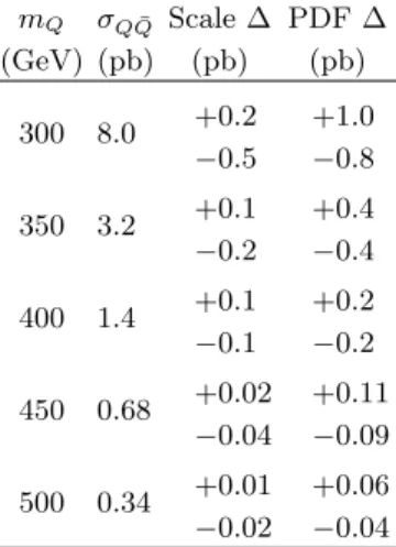
Production and decay of heavy-quark pairs (Q ¯Q) is modeled with the leading-order (LO) generator pythia 6.421 [18] using MRST 2007 LO* [19] parton distribu-tion funcdistribu-tions (PDFs). The producdistribu-tion cross-secdistribu-tion is calculated using hathor [20] with approximate next-to-next-to-leading-order (NNLO) QCD calculations with CTEQ6.6 PDFs [21] for several heavy-quark masses (mQ). In addition, scale uncertainties are evaluated in the range mQ/2 to 2×mQand PDF uncertainties are cal-culated from the CTEQ6.6 error eigenvectors. The cross-sections and uncertainties for each heavy-quark mass con-sidered in this analysis are shown in TableI. Samples are generated with either t0 → W b, t0 → W s, or t0 → W d final states; final results are verified with all three decay modes.
TABLE I. NNLO cross-sections, scale uncertainties and PDF uncertainties calculated using hathor for Q ¯Q production in √
s = 7 TeV pp collisions with CTEQ6.6 PDFs for different heavy-quark mass assumptions. Other uncertainties related to the cross-sections are neglected. The 1σ uncertainties are each represented by ∆. mQ σQ ¯Q Scale ∆ PDF ∆ (GeV) (pb) (pb) (pb) 300 8.0 +0.2 +1.0 −0.5 −0.8 350 3.2 +0.1 +0.4 −0.2 −0.4 400 1.4 +0.1 +0.2 −0.1 −0.2 450 0.68 +0.02 +0.11 −0.04 −0.09 500 0.34 +0.01 +0.06 −0.02 −0.04
B. Top quark pair production
The background due to t¯t production is modeled us-ing the next-to-leadus-ing-order (NLO) generator mc@nlo v3.41 [22] with an assumed top quark mass of 172.5 GeV and the NLO PDF set CTEQ6.6. The cross-section for t¯t production is normalized to the value obtained from an approximate NNLO calculation [20].
C. Z boson, diboson and single-top quark production
The background from Z/γ∗ boson production in asso-ciation with jets is modeled with the LO generator alp-gen v2.13 [23]. The LO PDF set CTEQ6.1 [21] is used to generate Z/γ∗+jets events with dilepton invariant mass m``> 10 GeV. For W W , W Z and ZZ production, events are generated with the LO generator herwig v6.5 and the LO PDF set CTEQ6.1. For the small background from single-top production, mc@nlo is used with the NLO PDF set CTEQ6.6, invoking the diagram removal scheme [24, 25] to remove overlaps between the single-top and t¯t final states. The cross-sections for Z/γ∗+jets samples are determined using NNLO inclusive calcula-tions from fewz [26, 27] and from a data-driven tech-nique where possible, while the cross-sections for dibo-son samples are determined using NLO calculations with mc@nlo. The cross-sections for single-top samples are normalized to an approximate NNLO prediction [28,29].
III. OBJECT SELECTION
Electrons are found by a calorimeter-seeded recon-struction algorithm and must have a track that matches an energy deposit in the calorimeter. They are re-quired to satisfy Ecluster/ cosh(ηtrack) > 25 GeV, where Ecluster is the energy deposited in the calorimeter clus-ter and ηtrack is the pseudorapidity of the matching track. Electrons are required to be in a pseudorapid-ity range |ηcluster| < 2.47, excluding the transition region 1.37 < |ηcluster| < 1.52 between the EM calorimeter bar-rel and endcap. They must also satisfy a calorimeter isolation Ical< 3.5 GeV requirement in ∆R < 0.2, where ∆R =p(∆η)2+ (∆φ)2. Calorimeter isolation is defined as the energy reconstructed within a cone of a certain radius around the lepton that is not associated with that lepton, and it is represented by Ical. The calorimeter shower shape is required to closely resemble what is ex-pected for electrons [10].
Jets are reconstructed from topological clusters of en-ergy deposits in the calorimeter [30] using the anti-kt algorithm with distance parameter R = 0.4 [31, 32]. These jets are calibrated to the hadronic energy scale us-ing a correction factor obtained from simulation which depends on pT and η [33] They are required to sat-isfy pT> 25 GeV and |η| < 2.5. Jets that fall within ∆R < 0.2 of accepted electrons are rejected.
Muons are found by requiring that a track recon-structed in the MS has a matching track in the ID. A loose cosmic ray rejection is applied by removing all muon pairs that are back-to-back azimuthally (∆φ(µ, µ0) > 3.1) and whose transverse impact parameter with respect to the beam line is greater than 0.5 mm. Muon can-didates must satisfy pT> 20 GeV and |η| < 2.5. The muon must be isolated, satisfying calorimeter isola-tion Ical< 4 GeV in ∆R < 0.3 and tracking isolation
Itrk< 4 GeV in ∆R < 0.3. Tracking isolation is defined as the sum of track momenta within a cone of a certain radius around the lepton vertex, and it is represented by Itrk. The muon must also not fall within ∆R < 0.4 of any jet with pT> 20 GeV.
The Emiss
T is constructed from the vector sum of calorimeter topological cluster energies projected onto the transverse plane [34]. Calorimeter deposits not asso-ciated to a jet are calibrated at the EM energy scale. De-posits associated with selected jets contribute at the cor-rected hadronic energy scale. Muon transverse momenta are included after correcting for muon energy losses in the calorimeters.
IV. BASELINE EVENT SELECTION
The Q ¯Q pair decay yields two charged leptons, two jets and EmissT from the undetected neutrinos. An ini-tial dilepton selection is applied to validate the modeling of the Z/γ∗boson production background as well as the identification of leptons, reconstruction of jets and mea-surement of Emiss
T .
The initial dilepton selection [35,36] first requires that an event contains a high-quality reconstructed primary vertex. The event must also have exactly two leptons (e or µ) with opposite charges, at least one of which must be associated with the object that triggered the event. The two leptons must not share a track in the ID. At this stage, the data sample is dominated by Z/γ∗ → `` de-cays (the Drell-Yan process), although the contribution from t¯t production is evident at large jet multiplicity, as can be seen in Figures1and2. These figures show good agreement between the data and background expecta-tion.
To reduce the background from Z/γ∗→ `` decays, the baseline selection requires:
• All events must have at least two jets, each with pT> 25 GeV and |η| < 2.5;
• Same-flavor events (ee and µµ) must satisfy a missing transverse momentum requirement, Emiss
T > 60 GeV;
• The dilepton invariant mass of same-flavor events (ee and µµ) must be greater than 15 GeV and must fall outside a window around the Z boson mass, defined as 81 GeV < m``< 101 GeV;
• In different-flavor events (eµ), HT, defined as the scalar sum of ETfrom every lepton and jet passing the object selection criteria, must exceed 130 GeV. The HTrequirement reduces the Z/γ∗→ τ τ back-ground, where a Emiss
T requirement is insufficient due to the presence of neutrinos.
jets N 0 2 4 6 8 10 Events 1 10 2 10 3 10 4 10 5 10 -1 L = 1.04 fb
∫
fake leptons single top
WW/WZ/ZZ tt τ τ → * γ Z/ Z/γ* → ee µ µ → * γ Z/ BG Uncertainty = 7 TeV) s Data ( ATLAS ee channel jets N 0 2 4 6 8 10 Events 1 10 2 10 3 10 4 10 5 10 (a) jets N 0 2 4 6 8 10 Events -1 10 1 10 2 10 3 10 4 10 5 10 6 10 7 10 -1 L = 1.04 fb
∫
fake leptons single top
WW/WZ/ZZ tt τ τ → * γ Z/ Z/γ* → ee µ µ → * γ Z/ BG Uncertainty = 7 TeV) s Data ( ATLAS channel µ µ jets N 0 2 4 6 8 10 Events -1 10 1 10 2 10 3 10 4 10 5 10 6 10 7 10 (b) jets N 0 2 4 6 8 10 Events 0 200 400 600 800 1000 -1 L = 1.04 fb
∫
fake leptons single top
WW/WZ/ZZ tt τ τ → * γ Z/ Z/γ* → ee µ µ → * γ Z/ BG Uncertainty = 7 TeV) s Data ( ATLAS channel µ e jets N 0 2 4 6 8 10 Events 0 200 400 600 800 1000 (c)
FIG. 1. Jet multiplicity after initial dilepton selection in (a) ee, (b) µµ, and (c) eµ channels. The shaded region indicates the magnitude of cross-section and luminosity uncertainties. Samples are stacked in the same order as they are presented in the legend, from left to right; the first entry in the legend is at the bottom of the stack. The data-driven Drell-Yan estimate defined in SectionV Ahas not been applied here.
[GeV] ll m 50 100 150 200 250 300 Events / 5 GeV 1 10 2 10 3 10 4 10 5 10 -1 L = 1.04 fb
∫
fake leptons single top
WW/WZ/ZZ tt τ τ → * γ Z/ Z/γ* → ee µ µ → * γ Z/ BG Uncertainty = 7 TeV) s Data ( ATLAS ee channel [GeV] ll m 50 100 150 200 250 300 Events / 5 GeV 1 10 2 10 3 10 4 10 5 10 (a) [GeV] ll m 50 100 150 200 250 300 Events / 5 GeV 1 10 2 10 3 10 4 10 5 10 -1 L = 1.04 fb
∫
fake leptons single top
WW/WZ/ZZ tt τ τ → * γ Z/ Z/γ* → ee µ µ → * γ Z/ BG Uncertainty = 7 TeV) s Data ( ATLAS channel µ µ [GeV] ll m 50 100 150 200 250 300 Events / 5 GeV 1 10 2 10 3 10 4 10 5 10 (b) [GeV] ll m 50 100 150 200 250 300 Events / 5 GeV 0 50 100 150 200 250 300 -1 L = 1.04 fb
∫
fake leptons single top
WW/WZ/ZZ tt τ τ → * γ Z/ Z/γ* → ee µ µ → * γ Z/ BG Uncertainty = 7 TeV) s Data ( ATLAS channel µ e [GeV] ll m 50 100 150 200 250 300 Events / 5 GeV 0 50 100 150 200 250 300 (c)
FIG. 2. Dilepton mass after initial dilepton selection in (a) ee, (b) µµ, and (c) eµ channels. The shaded region indicates the magnitude of cross-section and luminosity uncertainties. The last bin contains overflow events, and the first bin contains underflow events. Samples are stacked in the same order as they are presented in the legend, from left to right; the first entry in the legend is at the bottom of the stack. The data-driven Drell-Yan estimate defined in SectionV Ahas not been applied here.
V. DATA-DRIVEN ESTIMATES
A. Drell-Yan events
The total number of Drell-Yan ee and µµ events re-maining after the baseline selection has been applied is estimated with a data-driven technique that extrapolates from a control region (CR) [37]. Events in the CR have dilepton invariant mass in the range 81 GeV – 101 GeV with at least two jets and Emiss
T > 30 GeV. The number of data events in the control region, Data(CR), and MC Z/γ∗+jets events in the control region, MCDY(CR), are used to scale the prediction of Z/γ∗+jets events in the signal region, MCDY. Non-Z/γ∗ background processes in the control region, MCother(CR), are subtracted from the data using MC predictions. The estimated number of Z/γ∗+jets events in the signal region, NDY, in the ee and µµ channels is calculated with Equation1:
NDY =
(Data(CR) − MCother(CR)) MCDY(CR)
× MCDY. (1)
B. Fake lepton events
A small fraction of the background consists of events in which a jet or a non-prompt lepton is misidentified as a prompt lepton from W boson decay. Prompt lep-tons and misidentified non-prompt leplep-tons are referred to as real and fake leptons, respectively. Fake muons are predominantly produced from semi-leptonic b or c quark decays in which the muon passes the isolation re-quirements despite being produced in association with a jet. There are three principal mechanisms for producing fake electrons: heavy-flavor decay, light flavor jets with a leading π0overlapping with a reconstructed track from a charged particle, and asymmetric conversion of photons into e+e−. The largest source of events with fake leptons is W boson production with associated jets, including lepton plus jets decays of top quark pairs.
A matrix method [36] is used to estimate the fraction of the sample that comes from fake lepton events. A looser lepton selection is defined, and the number of observed dilepton events with two tight leptons (NTT), one loose and one tight lepton (NTL, NLT) or two loose leptons (NLL) is counted. The leptons are ordered by pT such that the leading lepton in NTL is tight and the leading lepton in NLT is loose. Tight leptons pass the selection criteria defined in Section III. Loose electrons need to pass the same selections as the electrons defined in Sec-tion III except for looser shower shape and calorimeter isolation requirements [10]. Loose muons only need to satisfy pT> 20 GeV, |η| < 2.5 and the muon-jet overlap requirements defined in SectionIII.
The probabilities for real and fake leptons that pass the loose identification criteria to also pass the tight criteria are defined as r`and f`, respectively. These two
probabil-ities are measured separately for ` = e and ` = µ. Using r`and f`, linear expressions are obtained for the observed yields as a function of the number of events with zero, one and two real leptons together with two, one and zero fake leptons (NFF, NRF and NFR, NRR; in NRF the real lepton has greater pTthan the fake lepton, and vice versa for NFR): NTT NTL NLT NLL = M NRR NRF NFR NFF , (2)
where M is a 4 × 4 matrix containing terms proportional to r` and f`. The matrix is inverted in order to extract the real and fake content of the observed dilepton event sample. The method explicitly accounts for the presence of events with two fake leptons.
The probability (r`) for a real loose lepton to pass the tight criteria is measured in Z → `` events in data with a tag-and-probe method. The probability for a fake loose electron to satisfy the tight requirements (fe) is measured by requiring exactly one loose electron in an event with Emiss
T < 10 GeV. The probability for a fake loose muon to satisfy the tight requirements (fµ) is mea-sured in a control region obtained by requiring exactly one loose muon with |∆φ(µ, Emiss
T )| < 0.5. The baseline selection requirements from SectionIV are not applied when checking these control regions.
VI. MASS RECONSTRUCTION
After the baseline selection has been applied, mass re-construction of heavy quark candidates is performed in order to discriminate the heavy-quark decays from the dominant t¯t background. Direct reconstruction is not possible, as two neutrinos escape the detector. However, a unique feature of the heavy quark is the large momen-tum of the daughter W boson, which makes its decay products approximately collinear in the detector as seen in Figure3.
Both neutrino momentum vectors are reconstructed by assuming that the neutrinos are the sole contribu-tors to ETmiss and that they are approximately collinear with the leptons. The optimal values of each |∆η(ν, `)| and each |∆φ(ν, `)| are fit by minimizing the mass differ-ence between the two reconstructed heavy quarks using minuit [38]. The fitted direction of each neutrino is con-strained to be within ∆R < 2.5 of the direction taken by the neutrino’s leptonic partner from the W boson decay, and all jet combinations are considered during each step of the mass difference minimization. A solution of the minimization procedure is penalized if the scalar sum of neutrino momenta exceeds the scalar sum of lepton mo-menta by at least 30%. The square of the difference be-tween each reconstructed W boson mass and 80.4 GeV is
added to the square of the heavy-quark mass difference in the minimized function; the preferred solutions pro-duce W bosons with reconstructed masses that are close to the W boson mass. The full minimization function is: fmin= (mQ1− mQ2) 2+ (m W1− (80.4 GeV)) 2+ (m W2− (80.4 GeV))2.
The two reconstructed mass values tend to be more correlated for signal than background, as shown in Fig-ure4. This is because the collinear approximation does not work well for single-top, diboson, Drell-Yan, and fake lepton events. An event is only kept if the two values of reconstructed mass are within 25 GeV of each other. The selection efficiency for this requirement is greater than 99% for each signal, 95% for t¯t, and only 75% – 90% for other backgrounds.
The final reconstructed mass (mCollinear) is taken to be the average of the two reconstructed masses in the event. Distributions of mCollinear for various simulated Q ¯Q samples and the t¯t background are shown in Figure5.
Generated Events 0 50 100 150 200 250 ) ν R(l, ∆ True 0 0.5 1 1.5 2 2.5 3 3.5 4 of W boson [GeV] T True p 0 50 100 150 200 250 300 350 400 450 500 Simulation ATLAS = 350 GeV Q m
FIG. 3. True pTof parent W boson versus true ∆R between
its daughter lepton and neutrino. The scale, shown on the right, indicates the number of generated MC events.
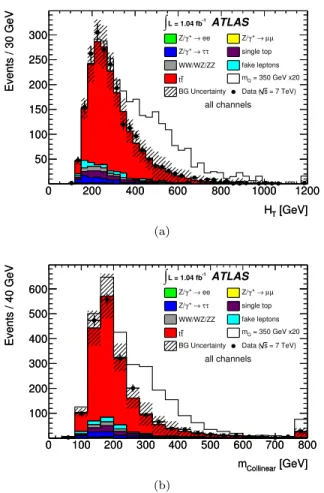
The expected background yields and number of ob-served events after the baseline selection are given in Ta-ble II. Distributions of HT and mCollinear are shown in Figure6.
VII. BACKGROUND VALIDATION
Event samples with the baseline selection and low HT, low lepton pT, low jet pT or low EmissT are examined to validate the modeling of the background (Figure 7). These conditions cause the distributions to be depleted of signal. In each case, the data is described well by the background model, within uncertainties.
[GeV] Collinear1 m 0 100 200 300 400 500 600 700 800 900 [GeV] Collinear2 m 0 200 400 600 800 1000 1200 1400 = 350 GeV Q m Background 25 GeV ± Collinear2 = m Collinear1 m Simulation ATLAS
FIG. 4. Correlation between reconstructed masses for Q ¯Q pairs produced with mQ = 350 GeV and for
background samples. The fitting method selects solu-tions with correlated mass values, however this correla-tion is smaller for background events. Events within |mCollinear1− mCollinear2| < 25 GeV are kept; this region is
found between the two lines in the figure.
[GeV]
Collinear
m
0 100 200 300 400 500 600 700 800
Fraction of Events / 40 GeV
0 0.05 0.1 0.15 0.2 0.25 0.3 Simulation ATLAS t t = 350 GeV Q m = 400 GeV Q m = 450 GeV Q m [GeV] Collinear m 0 100 200 300 400 500 600 700 800
Fraction of Events / 40 GeV
0 0.05 0.1 0.15 0.2 0.25 0.3
FIG. 5. mCollinearfor simulated heavy-quark pairs produced
with masses of 350 GeV, 400 GeV and 450 GeV and for top quark pairs. Each histogram is normalized to unit area. The distributions have long tails that are produced by wrong jet assignment in events where at least one of the correct jets fails selection requirements.
VIII. FINAL EVENT SELECTION
The baseline selection provides excellent discrimina-tion against Z/γ∗ production and other backgrounds, but additional selection requirements are necessary to suppress the dominant t¯t background. A tri-angular selection in HT + ETmiss versus mCollinear, HT+ ETmiss> X − 0.4 × mCollinear with X dependent on the assumed signal mass, is applied. Mass-dependent requirements on Emiss
T and leading jet pT are imposed as well. These selection requirements are optimized in MC simulation by seeking a point of maximum signif-icance, S/√S + B, while simultaneously varying all of
[GeV] T H 0 200 400 600 800 1000 1200 Events / 30 GeV 50 100 150 200 250 300 -1 L = 1.04 fb ∫ ee → * γ Z/ Z/γ* →µµ τ τ → * γ Z/ single top WW/WZ/ZZ fake leptons t t mQ = 350 GeV x20
BG Uncertainty Data (s = 7 TeV)
ATLAS all channels [GeV] T H 0 200 400 600 800 1000 1200 Events / 30 GeV 50 100 150 200 250 300 (a) [GeV] Collinear m 0 100 200 300 400 500 600 700 800 Events / 40 GeV 100 200 300 400 500 600 -1 L = 1.04 fb ∫ ee → * γ Z/ Z/γ* →µµ τ τ → * γ Z/ single top WW/WZ/ZZ fake leptons t t mQ = 350 GeV x20
BG Uncertainty Data (s = 7 TeV)
ATLAS all channels [GeV] Collinear m 0 100 200 300 400 500 600 700 800 Events / 40 GeV 100 200 300 400 500 600 (b)
FIG. 6. Expected and observed distributions of (a) HTand
(b) mCollinear for the sum of ee, µµ and eµ channels after
the baseline selection. The last bin contains overflow events. Samples are stacked in the same order as they are presented in the legend, from left to right; the first entry in the legend is at the bottom of the stack. The signal has been amplified to 20 times the expected rate.
TABLE II. Expected and observed number of events after baseline selection. Uncertainties shown are statistical and systematic, added in quadrature.
Process ee eµ µµ t¯t 190 +40−30 1140 +250 −200 370 +80 −70 single-top 9.4 +2.2 −1.9 60 +14−11 24 +5−5 Z/γ∗→ ee 6.3 +2.0−1.9 0.0 +0.1 −0.0 0.0 +0.1 −0.0 Z/γ∗→ µµ 0.0 +0.1−0.0 2.2 +1.1 −1.1 17 +5 −4 Z/γ∗→ τ τ 7.3 +2.4 −2.2 62 +15−12 16 +4−4 W W , W Z, ZZ 8.7 +2.2−1.9 49 +11 −10 12.7 +3.0 −2.6 fake leptons 3.7 ±2.8 70 ±40 0.5 ±0.8 Total Bg 230 +50−40 1380 +310 −250 440 +90 −80 Observed 243 1410 460 . [GeV] Collinear m 0 100 200 300 400 500 600 700 800 900 Events / 40 GeV 100 200 300 400 500 600 -1 L = 1.04 fb ∫ ee → * γ Z/ Z/γ* →µµ τ τ → * γ Z/ single top WW/WZ/ZZ fake leptons t t BG Uncertainty = 7 TeV) s Data ( ATLAS all channels < 400 GeV T H [GeV] Collinear m 0 100 200 300 400 500 600 700 800 900 Events / 40 GeV 100 200 300 400 500 600 (a) [GeV] Collinear m 0 100 200 300 400 500 600 700 800 900 Events / 40 GeV 50 100 150 200 250 -1 L = 1.04 fb ∫ ee → * γ Z/ Z/γ* →µµ τ τ → * γ Z/ single top WW/WZ/ZZ fake leptons t t BG Uncertainty = 7 TeV) s Data ( ATLAS all channels < 60 GeV T Leptons p [GeV] Collinear m 0 100 200 300 400 500 600 700 800 900 Events / 40 GeV 50 100 150 200 250 (b) [GeV] Collinear m 0 100 200 300 400 500 600 700 800 900 Events / 40 GeV 20 40 60 80 100 120 140 160 -1 L = 1.04 fb ∫ ee → * γ Z/ Z/γ* →µµ τ τ → * γ Z/ single top WW/WZ/ZZ fake leptons t t BG Uncertainty = 7 TeV) s Data ( ATLAS all channels < 60 GeV T Jets p [GeV] Collinear m 0 100 200 300 400 500 600 700 800 900 Events / 40 GeV 20 40 60 80 100 120 140 160 (c) [GeV] Collinear m 0 100 200 300 400 500 600 700 800 900 Events / 40 GeV 50 100 150 200 250 300 350 400 -1 L = 1.04 fb ∫ ee → * γ Z/ Z/γ* →µµ τ τ → * γ Z/ single top WW/WZ/ZZ fake leptons t t BG Uncertainty = 7 TeV) s Data ( ATLAS all channels < 80 GeV miss T E [GeV] Collinear m 0 100 200 300 400 500 600 700 800 900 Events / 40 GeV 50 100 150 200 250 300 350 400 (d)
FIG. 7. Distributions of mCollinear in events that have (a)
HT< 400 GeV, (b) two leptons with pT< 60 GeV, (c) all jets
with pT< 60 GeV or (d) ETmiss< 80 GeV. Each histogram
contains the sum of the ee, µµ and eµ channels. The last bin contains overflow events. Samples are stacked in the same order as they are presented in the legend, from left to right; the first entry in the legend is at the bottom of the stack.
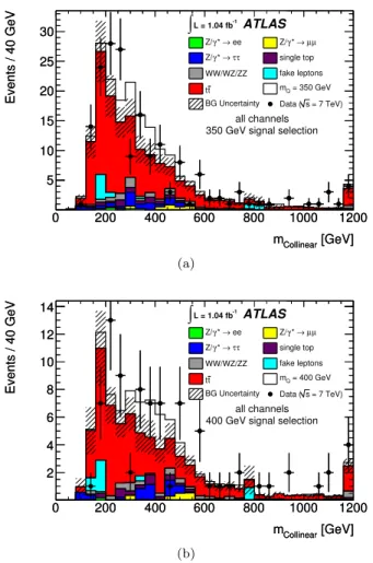
the selection requirement parameters. Distributions of HT + ETmiss versus mCollinear for background and signal are shown in Figure8. TablesIIIandIVlist the full set of optimized selection requirements at each mass point. TableV lists the expected backgrounds, expected signal and observed data for each mass point after this final se-lection. Figure9shows the distributions in mCollinear for two signal samples after the final selection.
Events 0 10 20 30 40 50 60 [GeV] Collinear m 0 100 200 300 400 500 600 [GeV] miss T + ET H 0 200 400 600 800 1000 Simulation ATLAS Backgrounds (a) Events 0 0.1 0.2 0.3 0.4 0.5 0.6 0.7 0.8 [GeV] Collinear m 0 100 200 300 400 500 600 [GeV] miss T + E T H 0 200 400 600 800 1000 Simulation ATLAS = 350 GeV Q m (b)
FIG. 8. HT+ ETmissversus mCollinearfor (a) background and
(b) mQ= 350 GeV signal events for the sum of ee, µµ, and eµ
channels. The scale, shown on the right, indicates the number of reconstructed MC events per bin passing the baseline selec-tion and weighted toR Ldt = 1.04 fb−1
. The shaded region is removed by the triangular selection requirement shown in TableIII.
IX. SYSTEMATIC UNCERTAINTIES
The major sources of systematic uncertainty are due to modeling of the signal and most sources of background.
The uncertainties due to simulation of the lepton trig-ger, reconstruction and selection efficiencies are assessed
TABLE III. List of HT+ ETmissversus mCollinearrequirements
for each mQ.
mQ(GeV) Triangle Requirement (GeV)
300 HT + ETmiss> 610 − 0.4 × mCollinear
350 HT + ETmiss> 700 − 0.4 × mCollinear
400 HT + ETmiss> 790 − 0.4 × mCollinear
450 HT + ETmiss> 880 − 0.4 × mCollinear
500 HT + ETmiss> 970 − 0.4 × mCollinear
TABLE IV. List of jet pT and ETmiss requirements for each
mQ.
mQ(GeV) Jet pT(GeV) ETmiss(GeV)
300 Leading jet pT> 80 —
350 Leading jet pT> 120 —
400 Leading jet pT> 130 ETmiss> 70
450 Leading jet pT> 130 ETmiss> 70
500 Leading jet pT> 130 ETmiss> 70
TABLE V. Expected background, expected signal and ob-served data in ee, µµ, and eµ channels for mQ= 300 − 500
GeV after final selection. The uncertainties shown include both statistical and systematic contributions.
mQ Expected Expected Observed
(GeV) Background Signal Data 300 300 +40−40 95 +14 −12 315 350 148 +22−18 35 +5 −4 180 400 75 +11−10 17.1 +2.5 −2.1 89 450 49 +8−6 8.4 +1.2 −1.0 57 500 30 +5 −4 4.4 +0.6 −0.5 36
using leptons from Z → ee and Z → µµ in data [36]. MC events are corrected for differences in data and sim-ulation. The statistical and systematic uncertainties in these corrections are included in the uncertainties on the acceptance values. Uncertainties in the modeling of the lepton energy scale and resolution are studied using re-constructed Z boson mass distributions. The jet energy scale (JES) and its uncertainty are derived by combining information from test-beam data, LHC collision data and simulation [33]. The JES uncertainty varies as a func-tion of jet pT and η and also accounts for the presence of nearby jets and event pileup. There is additional un-certainty associated with jets originating from b quarks in simulation. Smaller uncertainties are associated with the jet energy resolution and jet finding efficiency.
Uncertainties related to the Emiss
T arise due to uncer-tainties associated with low momenta jets, event pileup, and calorimeter energy not associated with reconstructed leptons or jets [34]. There is also some uncertainty in
[GeV] Collinear m 0 200 400 600 800 1000 1200 Events / 40 GeV 5 10 15 20 25 30 -1 L = 1.04 fb
∫
ee → * γ Z/ Z/γ* →µµ τ τ → * γ Z/ single top WW/WZ/ZZ fake leptons t t mQ = 350 GeVBG Uncertainty Data (s = 7 TeV)
ATLAS
all channels 350 GeV signal selection
[GeV] Collinear m 0 200 400 600 800 1000 1200 Events / 40 GeV 5 10 15 20 25 30 (a) [GeV] Collinear m 0 200 400 600 800 1000 1200 Events / 40 GeV 2 4 6 8 10 12 14 -1 L = 1.04 fb
∫
ee → * γ Z/ Z/γ* →µµ τ τ → * γ Z/ single top WW/WZ/ZZ fake leptons t t mQ = 400 GeVBG Uncertainty Data (s = 7 TeV)
ATLAS
all channels 400 GeV signal selection
[GeV] Collinear m 0 200 400 600 800 1000 1200 Events / 40 GeV 2 4 6 8 10 12 14 (b)
FIG. 9. Distributions of mCollinear for the sum of ee, µµ,
and eµ channels after applying the final selection for (a) mQ= 350 GeV and (b) mQ= 400 GeV. The last bin
con-tains overflow events. The uncertainty bands include all sta-tistical and systematic background uncertainties. The signal samples are normalized using the cross-sections in Table I. Samples are stacked in the same order as they are presented in the legend, from left to right; the first entry in the legend is at the bottom of the stack.
mating the effect of a readout problem affecting a subset of the LAr calorimeter channels in a part of the data set. The use of simulated samples to calculate the signal and background acceptances gives rise to systematic un-certainties from the generator choice, the amount of ini-tial and final state radiation (ISR/FSR), and from the PDF choice. The uncertainty due to the choice of gener-ator for t¯t events is evaluated by comparing the predic-tions of mc@nlo with those of powheg [39] interfaced to either herwig or pythia. The uncertainty due to ISR/FSR is evaluated by studies using the AcerMC [40] generator interfaced to pythia, varying the parameters controlling ISR and FSR in a range consistent with exper-imental data [41]. For Z/γ∗+jets events, the generator uncertainty is evaluated by comparing the predictions of alpgen with the PDF set CTEQ6.1 and sherpa [42] with the PDF set CTEQ6.6. Finally, the uncertainty in
TABLE VI. Overall normalization uncertainties for each back-ground, which are either due to cross-section uncertainties or uncertainties related to data-driven methods.
Background +1σ Unc. −1σ Unc.
t¯t 7 % 10 % single-top 7 % 7 % Z/γ∗→ ee 60 % 30 % Z/γ∗→ µµ 40 % 30 % Z/γ∗→ τ τ 40 % 40 % W W , W Z, ZZ 5 % 5 % fake leptons 50 % 50 %
the PDFs used to generate signal, t¯t and single-top events is evaluated using the procedure adopted in a measure-ment of the t¯t cross-section [36].
The integrated luminosity measurement carries a 3.7% uncertainty [16, 17]. Each sample also has an uncer-tainty associated with its theoretical cross-section or with its data-driven rate. For t¯t [20], single-top [28, 29] and Z/γ∗ → τ τ [43] the rate uncertainty is estimated from theoretical calculations. Z/γ∗ → ee, Z/γ∗ → µµ and fake lepton event rate uncertainties are evaluated with the data-driven fitting described in SectionV. The cross-section uncertainty for each signal point comes from hathor NNLO calculations and can be found in TableI. The background normalization uncertainties are listed in TableVI.
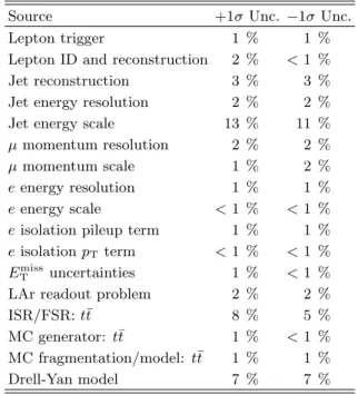
The effects of the systematic uncertainties on the over-all background yield are summarized in TableVIIfor the cuts used for mQ = 350 GeV.
X. RESULTS AND DISCUSSION
A binned maximum-likelihood ratio technique is used to fit distributions of mCollinear to the observed data in order to measure the most likely Q ¯Q production cross-section, σ(pp → Q ¯Q). In the fitting technique, all events with mCollinear> 760 GeV are considered to belong in the same bin. A shape fit is performed on background and signal simultaneously; this allows the background normalization to float, but maintains the bin-to-bin rela-tionships which defines the background and signal shapes in mCollinear. This fitting procedure allows for the possi-bility of an underestimated or overestimated background in the signal region. To take into account system-atic uncertainties, the signal and background shapes are smoothly deformed in generated samples of pseudo-data by random variations consistent with these uncertainties as shown in TableVIand Table VII; these fluctuations are not constrained by the data. Most of the systematic uncertainties are assumed to be correlated between signal and background; the uncertainties due to cross-section or data-driven estimates, Drell-Yan modeling, t¯t modeling,
TABLE VII. The effects of the ±1σ systematic uncertainties on the overall background yield.
Source +1σ Unc. −1σ Unc.
Lepton trigger 1 % 1 %
Lepton ID and reconstruction 2 % < 1 %
Jet reconstruction 3 % 3 %
Jet energy resolution 2 % 2 %
Jet energy scale 13 % 11 %
µ momentum resolution 2 % 2 %
µ momentum scale 1 % 2 %
e energy resolution 1 % 1 %
e energy scale < 1 % < 1 % e isolation pileup term 1 % 1 % e isolation pTterm < 1 % < 1 %
ETmissuncertainties 1 % < 1 %
LAr readout problem 2 % 2 %
ISR/FSR: t¯t 8 % 5 %
MC generator: t¯t 1 % < 1 % MC fragmentation/model: t¯t 1 % 1 %
Drell-Yan model 7 % 7 %
and t¯t generation are uncorrelated between signal and background.
A small excess is observed over the background expec-tation for each hypothetical Q mass.
Since the statistical interpretation uses the full shape of the signal and background distributions, the results the results in Table V do not entirely determine the re-sults; only a signal-like excess would weaken the observed limits. The excess shape in the mCollinear distribution is not particularly signal-like and the data are found to be in better agreement with the background-only than the signal+background hypothesis.
Statistical interpretation of the fitted cross-section σ is made using the CLs technique [44, 45]. This tech-nique performs fits in pseudo-data generated from the background model and varying levels of injected signal to measure the ability of the fit to distinguish between the background-only and background-plus-signal hypotheses. In the case that the data are in better agreement with the background-only hypothesis, 95% CL upper limits on the signal cross-section σ95are derived. The limit σ95 is chosen so that
ps 1 − p0
< 0.05
where psis the fraction of fits in pseudo-data with in-jected signal σ95 which give a result as seen in the data, and p0 is the corresponding fraction from pseudo-data drawn from the background hypothesis. Thus the per-formance of the fitting technique in ensembles of pseudo-data is naturally accounted for. Figure 10 shows the
observed and expected limits on the production cross-section σ(pp → Q ¯Q).
The upper limit on the production cross-section is converted into a lower limit on mQ by finding the point of intersection with the theoretical prediction as a function of mQ. This analysis finds a lower limit of mQ> 350 GeV at 95% confidence level (C.L.) whereas a limit of mQ> 335 GeV was expected. This limit as-sumes that the branching ratio (BR) of Q → W q is 100%. Limits were calculated for simulated samples of Q → W b, Q → W s, and Q → W d, but the results were approximately the same for all samples. The results from Q → W u and Q → W c were assumed to be analogous for Q → W s and Q → W d, respectively.
[GeV] Q m 300 320 340 360 380 400 420 440 460 480 500 ) [pb] q q -W + W → Q BR(Q× σ 1 10 2 10
∫
Ldt = 1.04 fb-1 95% C.L. NNLO from HATHORuncertainty σ 1 ± and
Median Expected Limit Observed Limit σ 1 ± σ 2 ± ATLAS [GeV] Q m 300 320 340 360 380 400 420 440 460 480 500 ) [pb] q q -W + W → Q BR(Q× σ 1 10 2 10
FIG. 10. Observed and median expected 95% C.L. cross-section upper limits on Q ¯Q production, compared to the the-oretical prediction. The limit was calculated for five signal masses, and a linear interpolation has been made between mass points. Limits were calculated for simulated samples of Q → W b, Q → W s, and Q → W d, but the results were approximately the same for all samples. The results from Q → W u and Q → W c were assumed to be analogous for Q → W s and Q → W d, respectively.
XI. CONCLUSIONS
This Article presents a search for pair production of heavy quarks decaying to W q in the dilepton channel at the CERN LHC. This search allows q = d, s, b for up-type Q final states or q = u, c for down-up-type Q final states. The analyzed data correspond to an integrated luminosity of 1.04 fb−1 collected by the ATLAS detector in pp collisions at √s = 7 TeV. To enhance the sensi-tivity to a new quark, mass reconstruction is performed by exploiting the boost received by the heavy-quark de-cay products. The reconstructed mass is used for binned maximum-likelihood ratio fitting.
The data are found to be in agreement with the ex-pectation from the Standard Model. A lower limit is set on the mass mQ> 350 GeV at 95% confidence level. This limit assumes BR(Q → W q) = 100% and is
appli-cable to many exotic models [46, 47], including up-type fourth-generation quarks t0, down-type fourth generation quarks b0, and quarks with exotic charges (such as −4/3) decaying to light quarks.
XII. ACKNOWLEDGEMENTS
We thank CERN for the very successful operation of the LHC, as well as the support staff from our institutions without whom ATLAS could not be operated efficiently. We acknowledge the support of ANPCyT, Argentina; YerPhI, Armenia; ARC, Australia; BMWF, Austria; ANAS, Azerbaijan; SSTC, Belarus; CNPq and FAPESP, Brazil; NSERC, NRC and CFI, Canada; CERN; CONI-CYT, Chile; CAS, MOST and NSFC, China; COLCIEN-CIAS, Colombia; MSMT CR, MPO CR and VSC CR, Czech Republic; DNRF, DNSRC and Lundbeck Founda-tion, Denmark; EPLANET and ERC, European Union; IN2P3-CNRS, CEA-DSM/IRFU, France; GNAS,
Geor-gia; BMBF, DFG, HGF, MPG and AvH Foundation, Germany; GSRT, Greece; ISF, MINERVA, GIF, DIP and Benoziyo Center, Israel; INFN, Italy; MEXT and JSPS, Japan; CNRST, Morocco; FOM and NWO, Netherlands; RCN, Norway; MNiSW, Poland; GRICES and FCT, Portugal; MERYS (MECTS), Romania; MES of Rus-sia and ROSATOM, RusRus-sian Federation; JINR; MSTD, Serbia; MSSR, Slovakia; ARRS and MVZT, Slovenia; DST/NRF, South Africa; MICINN, Spain; SRC and Wallenberg Foundation, Sweden; SER, SNSF and Can-tons of Bern and Geneva, Switzerland; NSC, Taiwan; TAEK, Turkey; STFC, the Royal Society and Lever-hulme Trust, United Kingdom; DOE and NSF, United States of America.
The crucial computing support from all WLCG part-ners is acknowledged gratefully, in particular from CERN and the ATLAS Tier-1 facilities at TRIUMF (Canada), NDGF (Denmark, Norway, Sweden), CC-IN2P3 (France), KIT/GridKA (Germany), INFN-CNAF (Italy), NL-T1 (Netherlands), PIC (Spain), ASGC (Tai-wan), RAL (UK) and BNL (USA) and in the Tier-2 fa-cilities worldwide.
[1] B. Holdom et al., PMC Phys. A 3, 4 (2009). [2] A. K. Alok et al., Phys. Rev. D 83, 073008 (2011). [3] The CDF Collaboration, Phys. Rev. Lett. 107, 261801
(2011).
[4] The CDF Collaboration, Phys. Rev. Lett. 106, 141803 (2011).
[5] The D0 Collaboration, Phys. Rev. Lett. 107, 082001 (2011).
[6] The ATLAS Collaboration, arXiv:1202.3076 (submitted to Phys. Rev. Lett.) (2012).
[7] The ATLAS Collaboration, arXiv:1202.6540 (submitted to Phys. Rev. Lett.) (2012).
[8] The ATLAS Collaboration, arXiv:1202.5520 (submitted to J. High Energy Phys.) (2012).
[9] The ATLAS Collaboration, JINST 3, S08003 (2008). [10] The ATLAS Collaboration, arXiv:1110.3174 (submitted
to Eur. Phys. J. C) (2011).
[11] G. Corcella et al., CERN-TH/2002-270 (2005).
[12] G. Corcella et al., J. High Energy Phys. 0101 (2001) 010. [13] J. M. Butterworth et al., Z. Phys. C 72, 637 (1996). [14] The GEANT4 Collaboration, Nucl. Instrum. Methods
Phys. Res., Sect. A 506, 250 (2003).
[15] The ATLAS Collaboration, Eur. Phys. J. C 70, 823 (2010).
[16] The ATLAS Collaboration, Eur. Phys. J. C 71, 1630 (2011).
[17] The ATLAS Collaboration, ATLAS-CONF-2011-116 (2011).https://cdsweb.cern.ch/record/1376384
[18] T. Sj¨ostrand et al., J. High Energy Phys. 0605 (2006) 026.
[19] A. Sherstnev and R. S. Thorne, Eur. Phys. J. C 55, 553 (2008).
[20] M. Aliev et al., Comput. Phys. Commun. 182:1034 (2011).
[21] P. M. Nadolsky et al., Phys. Rev. D 78, 013004 (2008).
[22] S. Frixione and B. R. Webber, J. High Energy Phys. 0206 (2002) 029.
[23] M. Mangano et al., J. High Energy Phys. 0307 (2003) 001.
[24] S. Frixione et al., J. High Energy Phys. 0807 (2008) 029. [25] S. Frixione et al., J. High Energy Phys. 0603 (2006) 092. [26] K. Melnikov and F. Petriello, Phys. Rev. D 74, 114017
(2006).
[27] R. Gavin et al., Comput. Phys. Commun. 182:2388 (2011).
[28] N. Kidonakis, Phys. Rev. D 83, 091503 (2011). [29] N. Kidonakis, Phys. Rev. D 81, 054028 (2010).
[30] W. Lampl et al., ATL-LARG-PUB-2008-002 (2008). https://cdsweb.cern.ch/record/1099735
[31] M. Cacciari, G. P. Salam and G. Soyez, J. High Energy Phys. 0804 (2008) 063.
[32] M. Cacciari and G. P. Salam, Phys. Lett. B 641 (2006) 57.
[33] The ATLAS Collaboration, arXiv:1112.6426 (submitted to Eur. Phys. J. C) (2011).
[34] The ATLAS Collaboration, Eur. Phys. J. C 72, 1844 (2012).
[35] The ATLAS Collaboration, ATLAS-CONF-2010-038 (2010).https://cdsweb.cern.ch/record/1277678
[36] The ATLAS Collaboration, Eur. Phys. J. C 71, 1577 (2011).
[37] The ATLAS Collaboration, ATLAS-CONF-2011-100 (2011).https://cdsweb.cern.ch/record/1369215
[38] F. James, CERN Program Library Long Writeup D506 (1998).
[39] P. Nason, PoS RADCOR2009 018 (2010). [40] B. Kersevan et al., TPJU-6/2004 (2004).
[41] The ATLAS Collaboration, CERN-OPEN-2008-020 (2009).
007.
[43] J. Alwall et al., Eur. Phys. J. C 53, 473 (2008). [44] A. Read, J. Phys. G 28, 2693 (2002).
[45] T. Junk, Nucl. Instrum. Methods Phys. Res., Sect. A
434, 435 (1999).
[46] J. A. Aguilar-Saavedra, J. High Energy Phys. 0911 (2009) 030.
The ATLAS Collaboration
G. Aad48, B. Abbott110, J. Abdallah11, A.A. Abdelalim49, A. Abdesselam117, O. Abdinov10, B. Abi111, M. Abolins87, O.S. AbouZeid157, H. Abramowicz152, H. Abreu114, E. Acerbi88a,88b, B.S. Acharya163a,163b, L. Adamczyk37, D.L. Adams24, T.N. Addy56, J. Adelman174, M. Aderholz98, S. Adomeit97, P. Adragna74, T. Adye128, S. Aefsky22, J.A. Aguilar-Saavedra123b,a, M. Aharrouche80, S.P. Ahlen21, F. Ahles48, A. Ahmad147, M. Ahsan40, G. Aielli132a,132b, T. Akdogan18a, T.P.A. ˚Akesson78, G. Akimoto154, A.V. Akimov93, A. Akiyama66, M.S. Alam1, M.A. Alam75, J. Albert168, S. Albrand55, M. Aleksa29, I.N. Aleksandrov64, F. Alessandria88a, C. Alexa25a, G. Alexander152, G. Alexandre49, T. Alexopoulos9, M. Alhroob20, M. Aliev15, G. Alimonti88a, J. Alison119, M. Aliyev10, B.M.M. Allbrooke17, P.P. Allport72, S.E. Allwood-Spiers53, J. Almond81,
A. Aloisio101a,101b, R. Alon170, A. Alonso78, B. Alvarez Gonzalez87, M.G. Alviggi101a,101b, K. Amako65,
P. Amaral29, C. Amelung22, V.V. Ammosov127, A. Amorim123a,b, G. Amor´os166, N. Amram152, C. Anastopoulos29, L.S. Ancu16, N. Andari114, T. Andeen34, C.F. Anders20, G. Anders58a, K.J. Anderson30, A. Andreazza88a,88b, V. Andrei58a, M-L. Andrieux55, X.S. Anduaga69, A. Angerami34, F. Anghinolfi29, A. Anisenkov106, N. Anjos123a, A. Annovi47, A. Antonaki8, M. Antonelli47, A. Antonov95, J. Antos143b, F. Anulli131a, S. Aoun82, L. Aperio Bella4, R. Apolle117,c, G. Arabidze87, I. Aracena142, Y. Arai65, A.T.H. Arce44, S. Arfaoui147, J-F. Arguin14, E. Arik18a,∗, M. Arik18a, A.J. Armbruster86, O. Arnaez80, C. Arnault114, A. Artamonov94, G. Artoni131a,131b, D. Arutinov20, S. Asai154, R. Asfandiyarov171, S. Ask27, B. ˚Asman145a,145b, L. Asquith5, K. Assamagan24, A. Astbury168, A. Astvatsatourov52, B. Aubert4, E. Auge114, K. Augsten126, M. Aurousseau144a, G. Avolio162, R. Avramidou9, D. Axen167, C. Ay54, G. Azuelos92,d, Y. Azuma154, M.A. Baak29, G. Baccaglioni88a, C. Bacci133a,133b, A.M. Bach14, H. Bachacou135, K. Bachas29, M. Backes49, M. Backhaus20, E. Badescu25a, P. Bagnaia131a,131b, S. Bahinipati2, Y. Bai32a, D.C. Bailey157, T. Bain157, J.T. Baines128, O.K. Baker174, M.D. Baker24, S. Baker76, E. Banas38,
P. Banerjee92, Sw. Banerjee171, D. Banfi29, A. Bangert149, V. Bansal168, H.S. Bansil17, L. Barak170, S.P. Baranov93, A. Barashkou64, A. Barbaro Galtieri14, T. Barber48, E.L. Barberio85, D. Barberis50a,50b, M. Barbero20,
D.Y. Bardin64, T. Barillari98, M. Barisonzi173, T. Barklow142, N. Barlow27, B.M. Barnett128, R.M. Barnett14, A. Baroncelli133a, G. Barone49, A.J. Barr117, F. Barreiro79, J. Barreiro Guimar˜aes da Costa57, P. Barrillon114, R. Bartoldus142, A.E. Barton70, V. Bartsch148, R.L. Bates53, L. Batkova143a, J.R. Batley27, A. Battaglia16, M. Battistin29, F. Bauer135, H.S. Bawa142,e, S. Beale97, T. Beau77, P.H. Beauchemin160, R. Beccherle50a, P. Bechtle20, H.P. Beck16, S. Becker97, M. Beckingham137, K.H. Becks173, A.J. Beddall18c, A. Beddall18c, S. Bedikian174, V.A. Bednyakov64, C.P. Bee82, M. Begel24, S. Behar Harpaz151, P.K. Behera62, M. Beimforde98, C. Belanger-Champagne84, P.J. Bell49, W.H. Bell49, G. Bella152, L. Bellagamba19a, F. Bellina29, M. Bellomo29, A. Belloni57, O. Beloborodova106,f, K. Belotskiy95, O. Beltramello29, S. Ben Ami151, O. Benary152,
D. Benchekroun134a, C. Benchouk82, M. Bendel80, N. Benekos164, Y. Benhammou152, E. Benhar Noccioli49, J.A. Benitez Garcia158b, D.P. Benjamin44, M. Benoit114, J.R. Bensinger22, K. Benslama129, S. Bentvelsen104, D. Berge29, E. Bergeaas Kuutmann41, N. Berger4, F. Berghaus168, E. Berglund104, J. Beringer14, P. Bernat76, R. Bernhard48, C. Bernius24, T. Berry75, C. Bertella82, A. Bertin19a,19b, F. Bertinelli29, F. Bertolucci121a,121b, M.I. Besana88a,88b, N. Besson135, S. Bethke98, W. Bhimji45, R.M. Bianchi29, M. Bianco71a,71b, O. Biebel97, S.P. Bieniek76, K. Bierwagen54, J. Biesiada14, M. Biglietti133a, H. Bilokon47, M. Bindi19a,19b, S. Binet114, A. Bingul18c, C. Bini131a,131b, C. Biscarat176, U. Bitenc48, K.M. Black21, R.E. Blair5, J.-B. Blanchard135, G. Blanchot29, T. Blazek143a, C. Blocker22, J. Blocki38, A. Blondel49, W. Blum80, U. Blumenschein54,
G.J. Bobbink104, V.B. Bobrovnikov106, S.S. Bocchetta78, A. Bocci44, C.R. Boddy117, M. Boehler41, J. Boek173, N. Boelaert35, J.A. Bogaerts29, A. Bogdanchikov106, A. Bogouch89,∗, C. Bohm145a, V. Boisvert75, T. Bold37, V. Boldea25a, N.M. Bolnet135, M. Bona74, V.G. Bondarenko95, M. Bondioli162, M. Boonekamp135, C.N. Booth138, S. Bordoni77, C. Borer16, A. Borisov127, G. Borissov70, I. Borjanovic12a, M. Borri81, S. Borroni86,
V. Bortolotto133a,133b, K. Bos104, D. Boscherini19a, M. Bosman11, H. Boterenbrood104, D. Botterill128, J. Bouchami92, J. Boudreau122, E.V. Bouhova-Thacker70, D. Boumediene33, C. Bourdarios114, N. Bousson82, A. Boveia30, J. Boyd29, I.R. Boyko64, N.I. Bozhko127, I. Bozovic-Jelisavcic12b, J. Bracinik17, A. Braem29, P. Branchini133a, G.W. Brandenburg57, A. Brandt7, G. Brandt117, O. Brandt54, U. Bratzler155, B. Brau83,
J.E. Brau113, H.M. Braun173, B. Brelier157, J. Bremer29, R. Brenner165, S. Bressler170, D. Britton53, F.M. Brochu27, I. Brock20, R. Brock87, T.J. Brodbeck70, E. Brodet152, F. Broggi88a, C. Bromberg87, J. Bronner98, G. Brooijmans34, W.K. Brooks31b, G. Brown81, H. Brown7, P.A. Bruckman de Renstrom38, D. Bruncko143b, R. Bruneliere48,
S. Brunet60, A. Bruni19a, G. Bruni19a, M. Bruschi19a, T. Buanes13, Q. Buat55, F. Bucci49, J. Buchanan117,
N.J. Buchanan2, P. Buchholz140, R.M. Buckingham117, A.G. Buckley45, S.I. Buda25a, I.A. Budagov64, B. Budick107, V. B¨uscher80, L. Bugge116, O. Bulekov95, M. Bunse42, T. Buran116, H. Burckhart29, S. Burdin72, T. Burgess13, S. Burke128, E. Busato33, P. Bussey53, C.P. Buszello165, F. Butin29, B. Butler142, J.M. Butler21, C.M. Buttar53, J.M. Butterworth76, W. Buttinger27, S. Cabrera Urb´an166, D. Caforio19a,19b, O. Cakir3a, P. Calafiura14,
G. Calderini77, P. Calfayan97, R. Calkins105, L.P. Caloba23a, R. Caloi131a,131b, D. Calvet33, S. Calvet33,
M. Campanelli76, V. Canale101a,101b, F. Canelli30,g, A. Canepa158a, J. Cantero79, L. Capasso101a,101b, M.D.M. Capeans Garrido29, I. Caprini25a, M. Caprini25a, D. Capriotti98, M. Capua36a,36b, R. Caputo80, C. Caramarcu24, R. Cardarelli132a, T. Carli29, G. Carlino101a, L. Carminati88a,88b, B. Caron84, S. Caron103, G.D. Carrillo Montoya171, A.A. Carter74, J.R. Carter27, J. Carvalho123a,h, D. Casadei107, M.P. Casado11, M. Cascella121a,121b, C. Caso50a,50b,∗, A.M. Castaneda Hernandez171, E. Castaneda-Miranda171,
V. Castillo Gimenez166, N.F. Castro123a, G. Cataldi71a, F. Cataneo29, A. Catinaccio29, J.R. Catmore29, A. Cattai29, G. Cattani132a,132b, S. Caughron87, D. Cauz163a,163c, P. Cavalleri77, D. Cavalli88a, M. Cavalli-Sforza11,
V. Cavasinni121a,121b, F. Ceradini133a,133b, A.S. Cerqueira23b, A. Cerri29, L. Cerrito74, F. Cerutti47, S.A. Cetin18b, F. Cevenini101a,101b, A. Chafaq134a, D. Chakraborty105, K. Chan2, B. Chapleau84, J.D. Chapman27,
J.W. Chapman86, E. Chareyre77, D.G. Charlton17, V. Chavda81, C.A. Chavez Barajas29, S. Cheatham84, S. Chekanov5, S.V. Chekulaev158a, G.A. Chelkov64, M.A. Chelstowska103, C. Chen63, H. Chen24, S. Chen32c, T. Chen32c, X. Chen171, S. Cheng32a, A. Cheplakov64, V.F. Chepurnov64, R. Cherkaoui El Moursli134e,
V. Chernyatin24, E. Cheu6, S.L. Cheung157, L. Chevalier135, G. Chiefari101a,101b, L. Chikovani51a, J.T. Childers29, A. Chilingarov70, G. Chiodini71a, A.S. Chisholm17, M.V. Chizhov64, G. Choudalakis30, S. Chouridou136,
I.A. Christidi76, A. Christov48, D. Chromek-Burckhart29, M.L. Chu150, J. Chudoba124, G. Ciapetti131a,131b, K. Ciba37, A.K. Ciftci3a, R. Ciftci3a, D. Cinca33, V. Cindro73, M.D. Ciobotaru162, C. Ciocca19a, A. Ciocio14, M. Cirilli86, M. Citterio88a, M. Ciubancan25a, A. Clark49, P.J. Clark45, W. Cleland122, J.C. Clemens82,
B. Clement55, C. Clement145a,145b, R.W. Clifft128, Y. Coadou82, M. Cobal163a,163c, A. Coccaro171, J. Cochran63, P. Coe117, J.G. Cogan142, J. Coggeshall164, E. Cogneras176, J. Colas4, A.P. Colijn104, N.J. Collins17,
C. Collins-Tooth53, J. Collot55, G. Colon83, P. Conde Mui˜no123a, E. Coniavitis117, M.C. Conidi11, M. Consonni103, V. Consorti48, S. Constantinescu25a, C. Conta118a,118b, F. Conventi101a,i, J. Cook29, M. Cooke14, B.D. Cooper76, A.M. Cooper-Sarkar117, K. Copic14, T. Cornelissen173, M. Corradi19a, F. Corriveau84,j, A. Cortes-Gonzalez164, G. Cortiana98, G. Costa88a, M.J. Costa166, D. Costanzo138, T. Costin30, D. Cˆot´e29, R. Coura Torres23a,
L. Courneyea168, G. Cowan75, C. Cowden27, B.E. Cox81, K. Cranmer107, F. Crescioli121a,121b, M. Cristinziani20, G. Crosetti36a,36b, R. Crupi71a,71b, S. Cr´ep´e-Renaudin55, C.-M. Cuciuc25a, C. Cuenca Almenar174,
T. Cuhadar Donszelmann138, M. Curatolo47, C.J. Curtis17, C. Cuthbert149, P. Cwetanski60, H. Czirr140, P. Czodrowski43, Z. Czyczula174, S. D’Auria53, M. D’Onofrio72, A. D’Orazio131a,131b, P.V.M. Da Silva23a, C. Da Via81, W. Dabrowski37, T. Dai86, C. Dallapiccola83, M. Dam35, M. Dameri50a,50b, D.S. Damiani136, H.O. Danielsson29, D. Dannheim98, V. Dao49, G. Darbo50a, G.L. Darlea25b, W. Davey20, T. Davidek125, N. Davidson85, R. Davidson70, E. Davies117,c, M. Davies92, A.R. Davison76, Y. Davygora58a, E. Dawe141, I. Dawson138, J.W. Dawson5,∗, R.K. Daya-Ishmukhametova22, K. De7, R. de Asmundis101a, S. De Castro19a,19b, P.E. De Castro Faria Salgado24, S. De Cecco77, J. de Graat97, N. De Groot103, P. de Jong104, C. De La Taille114, H. De la Torre79, B. De Lotto163a,163c, L. de Mora70, L. De Nooij104, D. De Pedis131a, A. De Salvo131a,
U. De Sanctis163a,163c, A. De Santo148, J.B. De Vivie De Regie114, S. Dean76, W.J. Dearnaley70, R. Debbe24, C. Debenedetti45, D.V. Dedovich64, J. Degenhardt119, M. Dehchar117, C. Del Papa163a,163c, J. Del Peso79, T. Del Prete121a,121b, T. Delemontex55, M. Deliyergiyev73, A. Dell’Acqua29, L. Dell’Asta21, M. Della Pietra101a,i, D. della Volpe101a,101b, M. Delmastro4, N. Delruelle29, P.A. Delsart55, C. Deluca147, S. Demers174, M. Demichev64, B. Demirkoz11,k, J. Deng162, S.P. Denisov127, D. Derendarz38, J.E. Derkaoui134d, F. Derue77, P. Dervan72,
K. Desch20, E. Devetak147, P.O. Deviveiros104, A. Dewhurst128, B. DeWilde147, S. Dhaliwal157, R. Dhullipudi24,l, A. Di Ciaccio132a,132b, L. Di Ciaccio4, A. Di Girolamo29, B. Di Girolamo29, S. Di Luise133a,133b, A. Di Mattia171, B. Di Micco29, R. Di Nardo47, A. Di Simone132a,132b, R. Di Sipio19a,19b, M.A. Diaz31a, F. Diblen18c, E.B. Diehl86, J. Dietrich41, T.A. Dietzsch58a, S. Diglio85, K. Dindar Yagci39, J. Dingfelder20, C. Dionisi131a,131b, P. Dita25a, S. Dita25a, F. Dittus29, F. Djama82, T. Djobava51b, M.A.B. do Vale23c, A. Do Valle Wemans123a, T.K.O. Doan4, M. Dobbs84, R. Dobinson29,∗, D. Dobos29, E. Dobson29,m, J. Dodd34, C. Doglioni49, T. Doherty53, Y. Doi65,∗, J. Dolejsi125, I. Dolenc73, Z. Dolezal125, B.A. Dolgoshein95,∗, T. Dohmae154, M. Donadelli23d, M. Donega119, J. Donini33, J. Dopke29, A. Doria101a, A. Dos Anjos171, M. Dosil11, A. Dotti121a,121b, M.T. Dova69, J.D. Dowell17, A.D. Doxiadis104, A.T. Doyle53, Z. Drasal125, J. Drees173, N. Dressnandt119, H. Drevermann29, C. Driouichi35, M. Dris9, J. Dubbert98, S. Dube14, E. Duchovni170, G. Duckeck97, A. Dudarev29, F. Dudziak63, M. D¨uhrssen29, I.P. Duerdoth81, L. Duflot114, M-A. Dufour84, M. Dunford29, H. Duran Yildiz3a, R. Duxfield138, M. Dwuznik37, F. Dydak29, M. D¨uren52, W.L. Ebenstein44, J. Ebke97, S. Eckweiler80, K. Edmonds80, C.A. Edwards75, N.C. Edwards53, W. Ehrenfeld41, T. Ehrich98, T. Eifert142, G. Eigen13, K. Einsweiler14, E. Eisenhandler74, T. Ekelof165, M. El Kacimi134c, M. Ellert165, S. Elles4, F. Ellinghaus80, K. Ellis74, N. Ellis29, J. Elmsheuser97, M. Elsing29, D. Emeliyanov128, R. Engelmann147, A. Engl97, B. Epp61, A. Eppig86, J. Erdmann54, A. Ereditato16, D. Eriksson145a, J. Ernst1, M. Ernst24, J. Ernwein135, D. Errede164, S. Errede164, E. Ertel80, M. Escalier114, C. Escobar122, X. Espinal Curull11, B. Esposito47, F. Etienne82, A.I. Etienvre135, E. Etzion152, D. Evangelakou54, H. Evans60, L. Fabbri19a,19b, C. Fabre29, R.M. Fakhrutdinov127, S. Falciano131a, Y. Fang171, M. Fanti88a,88b, A. Farbin7, A. Farilla133a, J. Farley147, T. Farooque157, S.M. Farrington117, P. Farthouat29, P. Fassnacht29, D. Fassouliotis8, B. Fatholahzadeh157, A. Favareto88a,88b, L. Fayard114, S. Fazio36a,36b, R. Febbraro33,