Measuring complexity in a business cycle
Texto
Imagem

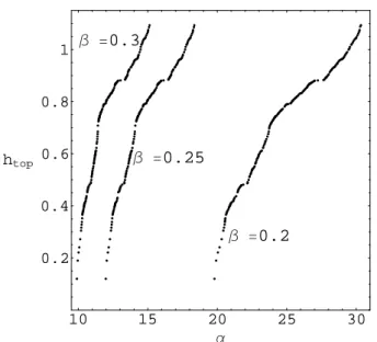
![Fig. 6. Bifurcation diagram of the map f for α ∈ [15, 30] , β = 0.2, c = 0.75 and γ = 1.65](https://thumb-eu.123doks.com/thumbv2/123dok_br/15731799.1071571/13.892.280.591.126.335/fig-bifurcation-diagram-map-f-α-β-γ.webp)

Documentos relacionados
The paper is organized as follows: Section II introduces our signal model and some basic equations concerning the computation of 4th-order cumulants; in Section III we express
5 Conferir anexo I.. 17 não faziam parte da lista dos educandos indicados. Foram selecionados a partir de tal avaliação, 37 educandos que não conseguiram um rendimento
∑ Os fornos microondas podem não cozinhar os alimentos uniformemente permitindo zonas frias onde as bactérias perigosas podem sobreviver. Assegure-se que os
The present paper was organized in four sections: in section 1 we introduced the study; in section 2 we actualized the revision of the literature of AQUA-motion domain presenting:
Após análise do SF-36 nos domínios Dor relacionando Aspectos físicos, foi possível verificar que os resultados foram semelhantes entre os indivíduos estudados, visto que
Ao verificar a média de conhecimento dos alunos segundo a instituição e níveis do perfil do aluno, observa-se que em todos os níveis o aluno da escola pública apresentou maior
que se traduziu na condenação do Estado português no pagamento de uma sanção pecuniária compulsória diária de 19 392,00€ 75 , em resultado da postura do legislador
