eve cerfernandes tensor

(1)

Tensor-based blind channel identification

Carlos Estˆev˜ao R. Fernandes

I3S Laboratory

University of Nice Sophia Antipolis Sophia Antipolis, France, 06903

Email: cfernand@i3s.unice.fr

G´erard Favier

I3S Laboratory

University of Nice Sophia Antipolis Sophia Antipolis, France, 06903

Email: favier@i3s.unice.fr

Jo˜ao Cesar M. Mota

Teleinformatics Engineering Department Federal University of Cear´a Fortaleza, Cear´a, Brazil 60455-760

Email: mota@deti.ufc.br

Abstract— We propose a blind FIR channel identification method based on the Parallel Factor (Parafac) analysis of a 3rd-order tensor composed of the 4-th order output cumulants. Our algorithm is based on a single-step least squares (LS) minimization procedure instead of using classical three-step Alternating Least Squares (ALS) methods. Using a Parafac-based decomposition, we avoid any kind of pre-processing such as the prewhitening operation, which is mandatory in most methods using higher-order statistics. Our method retrieves the channel vector without any permutation or scaling ambiguities. In addition, we establish a link between the cumulant tensor decomposition and the joint-diagonalization approach. Computer simulations illustrate the performance gains that our method provides with respect to other classical solutions. Initialization and convergence issues are also addressed.

I. INTRODUCTION

Blind channel identification and equalization consist in the retrieval of unknown information about the transmission channel and source signals from the knowledge of the received signal only. For several years, higher-order statistics (HOS) have been an important research topic in diverse fields includ-ing data communication, speech and image processinclud-ing and geophysical data processing. The higher-order spectra have the ability to preserve both magnitude and (nonminimum-) phase information. Moreover, it is well-known that all cumulant spectra of order greater than 2 vanish for Gaussian signals, which makes HOS-based identification methods insensitive to an additive Gaussian noise.

Relationships connecting different higher-order cumulant slices and the parameters of a finite impulse response (FIR) model exist and it is well known that larger sets of output cu-mulants have the ability to improve identification performance [1]. Existing approaches to exploit the sample output cumu-lants include the joint-diagonalization of cumulant matrices [2]. However, such techniques involve aprewhitening transfor-mation over the cumulant matrices, which is often a source of increased complexity and estimation errors. The factorization of third-order tensors containing sample 4th-order cumulants has the advantage of avoiding the prewhitening operation by fully exploiting the three-dimensional nature of the cumulant tensor.

The Parallel factor analysis (Parafac) of an m-dimensional tensor with rankF consists in the decomposition of the tensor into a sum ofF factors where each factor can be written as the outer product of m vectors [3]. The trilinear Parafac model

(m = 3) has become very popular in the fields of Psycho-metrics and ChemoPsycho-metrics [4], [5] but it also has been widely used in Signal Processing applications [6], [7]. The key-point in the use of the Parafac is about its uniqueness property, which can be assured under simple conditions that are stated in the Kruskal Theorem [8]. Among many algorithms to fit the Parafac model, the Alternating Least Squares (ALS) algorithm is one of the most popular ones, despite its known problems concerning complexity, convergence speed and non-guaranteed convergence to the global minimum.

In this paper, we exploit the high symmetry of the 4th-order cumulants to propose a solution based on a single-step least squares (LS) minimization procedure. We recover the parameters of an FIR channel by means of the Parafac decomposition of a three-dimensional tensor containing the output 4th-order cumulants. The uniqueness issue is also addressed and we present computer simulations comparing our method with the joint-diagonalization based approach as well as with the (closed-form) Total Least Squares (TLS) solution. Initialization and convergence speed are discussed and we show that our method can be used to improve the TLS solution. The paper is organized as follows: Section II introduces our signal model and some basic equations concerning the computation of 4th-order cumulants; in Section III we express the output cumulants as a three-dimensional tensor and show that it consists in a Parafac model; in Section IV we present the equations for the cumulant tensor decomposition and show that there is a direct link with the matrix diagonalization approach; in Section V we propose a simplified Parafac-based algorithm to estimate channel parameters; Section VI presents some illustrative computer simulation results and Section VII finally draws some conclusions and perspectives.

II. SIGNAL MODEL AND OUTPUT CUMULANTS

We start considering the baseband representation of a dig-italsingle-input single-output (SISO) communication channel where the output signaly(n)after sampling at the symbol rate is written as follows:

y(n) =x(n) +υ(n),

x(n) = L

l=0

hls(n−l), (1)

where h0 = 1, which is equivalent to a simple unit-norm

(2)

A1 : The non-measurable, complex-valued, discrete input se-quences(n)is non-Gaussian, stationary, independent and identically distributed (i.i.d. ) with symmetric distribution of zero-mean and variance σ2

s = 1.

A2 : The additive Gaussian noise sequence υ(n) has zero-mean and is independent from s(n). Its autocorrelation function is unknown.

A3 : The channel frequency-response isH(ω) =

lhle−jωl with complex coefficients hl representing the equivalent discrete impulse response, including the pulse shaping filter, the channel itself and the receiving filter.

A4 : The system is causal with memoryL, i.e.hl= 0, ∀l /∈ [0, L]. In addition, hL= 0 andL= 0.

The output 4th-order cumulants will be defined as follows

c4,y(τ1, τ2, τ3)cum

y∗(n), y(n+τ1), y∗(n+τ2), y(n+τ3)

.

Using the channel model (1), taking assumptions A1 and A2 into account, and making use of the multilinearity property of cumulants, it is easy to show that [9]:

c4,y(τ1, τ2, τ3) =γ4,s L

l=0

h∗ lhl+τ1h

∗

l+τ2hl+τ3, (2)

where γ4,s = c4,s(0,0,0). Based on (2) and on assumption

A4, it is easy to verify that

c4,y(τ1, τ2, τ3) = 0,∀ |τ1|,|τ2|,|τ3|> L. (3)

Hence, making the time-lagsτ1,τ2andτ3vary in the interval [−L, L] we get all the nonzero values of c4,y(τ1, τ2, τ3).

Such a choice allows us to construct a maximal redundant information model, in which the 4th-order cumulants are taken for time-lags τ1,τ2 andτ3 within the interval[−L, L].

III. TENSOR FORMULATION

Let us define the three-dimensional tensor C(4,y) _∈

C(2L+1)×(2L+1)×(2L+1)_{, in which the element in position} (i, j, k) corresponds to c4,y(i, j, k), with i = τ1 +L+ 1,

j = τ2+L+ 1 and k = τ3+L+ 1, as shown in Figure

1a. Therefore,C(4,y) _{is clearly a 3rd-order tensor represented}

as a cube of dimensions(2L+ 1)×(2L+ 1)×(2L+ 1)and it can be written as:

C(4,y)₌ 2L+1

i=1 2L+1

j=1 2L+1

k=1

Cijk e(2 L+1)

i ◦e

(2L+1)

j ◦e

(2L+1)

k (4)

where Cijk = c4,y(i−L−1, j −L−1, k −L−1), the

symbol ◦ stands for the outer product and e(_pP) _{denotes the}

p-th canonical basis vector with dimensionP [10]. Replacing (2) in (4) we can easily write the tensor C(4,y) _{as a sum of}

L+ 1outer products, each one involving exactly 3 vectors, as follows:

C(4,y)₌_γ 4,s

L

l=0

h∗ lh.l◦h

∗

.l◦h.l (5)

where h_.l ₌ 2L+1

p=1 hl+p−L−1e(2pL+1). The above nota-tion leads us to define the channel coefficient matrix H _∈

C(2L+1)×(L+1)_{as follows:}

H _H_h

=h_.₀ h_.₁_{. . .}h_.L

= 

          

0 0 · · · h0

..

. ... . .. ... 0 h0 · · · hL−1

h0 h1 · · · hL ..

. ... . .. ...

hL−1 hL · · · 0

hL 0 · · · 0 

          

(6)

whereH ·

is an operator that builds a special Hankel matrix from the vector argument as shown above and the channel coefficients vector is:

h₌_h₀_{. . . h}_LT _∈C(L+1)_. ₍₇₎

IV. CUMULANT TENSOR DECOMPOSITION

Slicing tensor C(4,y) _{along the three possible directions}

(horizontal, vertical and frontal) yields in each case 2L+ 1 matrices of dimensions(2L+1)×(2L+1). Figure 1b illustrates frontal slicing fork∈[1,2L+ 1]. The two-dimensional slices obtained from each direction will be denoted C(4_i..,y)_,C(4_.j.,y)

andC(4,y)

..k withi, j, k∈[1,2L+ 1], respectively. SlicingC(4,y)_{along the frontal direction we get:}

C(4,y)

..k = 2L+1

i=1 2L+1

j=1

Cijke (2L+1)

i e

(2L+1)T

j

= γ4,s L

l=0

h∗

lhl+k−L−1h.lhH.l

and then

C(4,y)

..k =γ4,sHDk(Σ)HH, (8) for allk∈[1,2L+ 1], whereDp(·)is an operator that forms a diagonal matrix with the main diagonal constituted by the elements of thep-th row of the matrix argument and:

Σ₌HDiag(h∗

) ∈C(2L+1)×(L+1)

(9)

where theDiag(·)operator builds a diagonal matrix using the entries of the vector argument, so Dk(Σ) ∈ C(L+1)×(L+1). Slicing C(4,y) _{along the vertical direction, we get:}

C(4_.j.,y) ₌ 2L+1

i=1 2L+1

k=1

Cijke (2L+1)

i e

(2L+1)T

k

= γ4,s L

l=0

h∗ lh

∗

l+j−L−1h.lhT.l

and then

C(4_.j.,y) ₌ _γ₄_,sHDiag(h∗

)Dj(H∗)HT

(3)

c

( ,

, )

4, y

C

(4, y) ..k

2 1

3

= –L = L

= k – L – 1

τ

1

τ

3

τ

2

τ

3

τ

3

τ

3

τ

1

τ

₂ 3

τ

(a) (b)

Fig. 1. (a) Three-dimensional cumulant tensorC(4,y)_{composed of the 4th-order output cumulants; (b) frontal slices of tensor}_C(4,y)_.

for all j∈[1,2L+ 1]. Finally, taking the horizontal direction and following the same reasoning, we can easily write:

C(4,y)

i.. = 2L+1

j=1 2L+1

k=1

Cijke (2L+1)

j e

(2L+1)T

k

= γ4,s L

l=0

h∗

lhl+i−L−1h∗.lhT.l

= γ4,sH ∗

Di(H)Diag(h ∗

)HT

= γ4,sH ∗

Di(H)ΣT, (11)

for alli∈[1,2L+ 1].

In particular, equation (8) establishes a direct link between the tensor decomposition and the joint-diagonalization ap-proach [2]. However, diagonalization procedures of the type

A₌UDUH _require U _{to be unitary, i.e.} UUH ₌I_{. In our}

case, since H _{is not unitary, the diagonalization of matrices}

in (8) for k ∈ [1,2L+ 1] is not possible without a previ-ous orthonormalization step in which a new set of modified cumulant matrices is constructed as C¯(4,y)

..k =WC (4,y) ..k WH, with WH_{unitary. Matrix} W_{is often referred to as the} pre-whiteningfactor and its computation usually requires resorting to second-order statistics (SOS). This additional step, very common in most HOS-based methods, is time-consuming and often responsible for increased estimation errors.

It is important to express the cumulant tensor in an unfolded tensor representation, obtained by stacking up the 2D slices. Three unfolded representations ofC(4,y)_{are possible. Stacking}

up matricesC(4,y)

..k for k∈[1,2L+ 1], we get:

C_[3]₌



  

C(4_..,y) 1

.. .

C(4,y)

..(2L+1) 

  

=γ4,s 

 

H_D₁₍Σ₎

.. .

H_D₂_L₊₁₍Σ₎



 H

H

hence

C_[3]₌_γ₄_,sΣ_⋄HHH_, ₍₁₂₎

where ⋄ stands for the Khatri-Rao product. We also get:

C_[2]₌_γ₄_,sH∗

⋄ΣHT ₍₁₃₎

from (10) and finally

C_[1]₌_γ₄_,sH_⋄H∗

ΣT ₍₁₄₎

from (11). Table I resumes the information about the Parafac decomposition of tensorC(4,y) _{highlighting the formulae}

de-veloped above. Equations (12)−(14) can be used to estimate matricesH_andΣ_{and thus the channel parameters. However,}

we can simplify the estimation ofh_{by taking the relationships}

between the channel coefficient vector and the matricesH_and Σ _{into account, thus eliminating the ambiguities.}

TABLE I

PARAFACFORMULAE FOR THE3RD-ORDER TENSORC(4,y)_.

Direction Tensor 2D slices Unfolded representations

Horizontal C(4,y)

i.. =γ4,sH∗Di(H)ΣT C[1]=γ4,s

H⋄H∗ΣT

Vertical C(4,y)

.j. =γ4,sΣDj(H∗)HT C[2]=γ4,s

H∗⋄ΣHT

Frontal C(4,y)

..k =γ4,sHDk(Σ)HH C[3]=γ4,s

Σ⋄HHH

The uniqueness issue

The great importance of Parafac is mostly due to the simple conditions that assure its uniqueness, for tensors of order higher than 2. A sufficient uniqueness condition is stated by the Kruskal Theorem [8]. For the case of the 3rd-order tensor C(4,y)_{, the Kruskal Theorem states that the Parafac}

decomposition is unique up to column scaling and permutation ambiguities if:

2kH+kΣ≥2(L+ 1), (15)

where kH is the k-rank of the channel matrix H. The k -rank of an n ×m matrix X_{, denoted by} _k_X_{, stands for}

the largest integer kX for which every set containing kX columns ofX _{is independent. From this definition, note that}

kX ≤rX ≤ min(n, m). Several authors have addressed the Parafac uniqueness problem and different proofs have been given to the Kruskal Theorem [8], [5].

Due to its Hankel structure and assumption A4, matrix H

(4)

assumption A4, we conclude that Σ _{is also full-rank so that}

kΣ=rΣ=L+ 1and hence 2kH+kΣ= 3L+ 3. So, from

(15) we conclude that the Kruskal uniqueness condition is always satisfied under the considered assumptions. Therefore, the Parafac decomposition of C(4,y) _{is unique up to column}

scaling and permutation ambiguities.

In the next section, we show that it is possible to avoid the computation of the pre-whitening factor and estimate H

without an orthonormalization step. We propose a single-step least squares (LS) algorithm to estimate vector h _{by means}

of the above described tensor decomposition, instead of using a diagonalization approach. Exploiting the Hankel structure of H _{and the system constraint} _h₀ _{= 1}_{, no permutation nor}

scaling ambiguities remain in the model. Making use of the symmetries of the 4th-order cumulants and of some Khatri-Rao product properties, we eliminate the need for estimating

H _{prior to}h_.

V. PARAFAC-BASEDBLINDCHANNELIDENTIFICATION ALGORITHM

In order to estimate the channel coefficients without having to computeH_andΣ_{we make use of relationships (6) and (9)}

and, based on the following property of the Khatri-Rao product [11], we propose an iterative Least Squares (LS) procedure to estimate vector h_.

Property 1 If matrices A _∈ Cm×n _and _B _∈ _Cn×m _and

vector d_∈Cn _{are such that}_X₌_A_Diag₍_d₎_B_{, then it holds}

vecX=

BT_⋄Ad ₍₁₆₎

where vec·stands for the vectorizingoperator.

Note from table I that, among the three unfolded matrices,

C_[1] _{is the most suitable representation to apply Property 1.}

That is because we can rewrite (14) as follows:

C_[1]₌_γ₄_,sH_⋄H∗

Diag(h∗ )HT

and thus, using (16), it is straightforward to write:

vecC_[1]=γ₄_,sH⋄H⋄H∗h∗. (17)

The channel coefficients vector h _{can be obtained by}

minimizing the following least squares (LS) cost function:

Jh∗

vec

C_[1]₋Gˆ(r−1)_h∗ 2

F (18)

by means of an iterative procedure, where:

ˆ

G(r−1)₌_γ₄_,sHˆ(r−1)_⋄Hˆ(r−1)_⋄Hˆ(r−1)∗

. (19)

The algorithm is initialized with a Hankel matrix Hˆ(0) _in

which the first column is [0T

(L) hˆ

(0)T_]T _{and the last row is}

[ˆh(0)L 0T(L)], wherehˆ

(0)_{= [1} _vT_]T _andv_∈C(L)_{is a Gaussian}

random vector. The algorithm iterates until convergence of the parametric estimator, i.e. until hˆ(r)₋_h_ˆ(r−1)_/_h_ˆ(r)_≤_ε_,

where r is the iteration number and ε is an arbitrary small

positive constant. At each iteration r, we use the estimate ˆ

h(r−1) _{to update}Hˆ(r−1)_.

Our strategy ensures the Hankel structure of H _{at each}

iteration, taking advantage of its full-rank property to make the tensor decomposition essentially unique and free from permutation ambiguities. The constrainth0= 1 is taken into

account in the construction of hˆ(r) _{in order to avoid any}

kind of scaling ambiguities. Furthermore, a single-step LS minimization procedure is used instead of the classical three-step alternating least squares (ALS) algorithm. For this reason, our method should be expected to increase convergence speed. Finally, this approach is shown to provide an improved solu-tion at each new iterasolu-tion and if it converges to the global minimum, the LS solution to the model is found [3].

After initializing hˆ(0) _{as a Gaussian random vector, the}

algorithm to estimate the channel coefficients vector can be summarized as follows, forr≥1:

1) Use (6) to buildHˆ(r−1)₌_Hhˆ(r−1)_;

2) Using (19), computeGˆ(r−1)_;

3) Minimize the cost function (18) so that ˆ

h(r)∗ =γ−1

4,sGˆ

(r−1)#_vec

C_[1] ₍₂₀₎

where(·)#_{stands for the}_{Moore-Penrose}_{pseudoinverse,}

computed from the singular value decomposition (SVD) of its matrix argument.

4) Reiterate until convergence of the parametric error, i.e. hˆ(r)₋_h_ˆ(r−1)_/_h_ˆ(r)_≤_ε_.

Next, we will present some computer simulations illus-trating the applicability of the proposed Parafac-based Blind Channel Identification(PBCI) method.

VI. COMPUTER SIMULATIONS

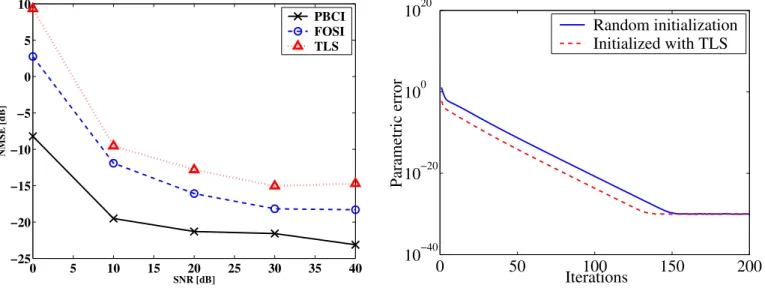
In this section, our results are compared with those ob-tained from the well-known Fourth-Order System Identifi-cation (FOSI) algorithm, which is based on a joint diag-onalization technique. As suggested by the authors of this latter method, the FOSI algorithm performance is obtained by averaging the results of the two solutions proposed in [2]. In addition, we also compare PBCI results with the optimal algebraic solution in the total least squares (TLS) sense, proposed in [1]. In order to further assess the performance of our methods, other algorithms proposed in the literature should be used in the future, such as the FIR system identification proposed in [12].

Parametric channel estimation performance is evaluated by means of the normalized mean squared error (NMSE) of the estimator, which is computed through the following formula:

NMSE₌ 1

P

p=1 hˆ(∞)

p −h2

h2 , (21)

where P is the number of Monte Carlo runs andhˆ(∞) p is the channel estimate obtained after convergence of the experiment

p∈[1, P].

(5)

0 5 10 15 20 25 30 35 40 −25

−20 −15 −10 −5 0 5 10

SNR [dB]

NMSE [dB]

PBCI FOSI TLS

Fig. 2. Identification performances of PBCI, FOSI and TLS methods with QPSK modulation.

That can be observed in Figure 2, where the NMSE is plotted against signal-to-noise ratio (SNR) for PBCI, FOSI and TLS algorithms. These curves represent the average of

P = 50 Monte Carlo runs and channel parameter vector equals h_{= [1}_, ₁_.₃₇₋₁_.₁₂_i, ₀_.₉₄₋₀_.₇₅_i_]T ₍_L_{= 2}_). Fourth-order cumulants were estimated fromN = 10000output data samples assuming perfect knowledge of the channel memory

L.

We also show that the number of iterations required for convergence of our Parafac-based algorithm can be reduced by initializing PCBI with the TLS solution. Figure 3 illustrates this situation, showing that this new initialization condition yields the same steady state results as before , but requires less iterations. This can be viewed as a way to improve the TLS solution over a limited number of iteration steps.

VII. CONCLUSIONS AND PERSPECTIVES

This paper has presented a new blind FIR channel identifica-tion method based on the Parafac decomposiidentifica-tion of a 3rd-order tensor composed of 4th-order output cumulants. Our method fully exploits the three-dimensional nature of the cumulant tensor and has the advantage of avoiding any kind of pre-processing. Moreover, our tensor decomposition algorithm is based on a single-step LS procedure instead of the classical three-step alternating least squares (ALS) algorithm. Unique-ness and convergence issues have been addressed. Computer simulations show that the Parafac-based approach provides better estimation performance than both the (closed-form) TLS solution and the joint-diagonalization based algorithm. Furthermore, the convergence of the PBCI algorithm can be accelerated when it is initialized with the TLS solution

0

50

100

150

200

10

−40

10

−20

10

0

10

20

Iterations

Parametric error

Random initialization

Initialized with TLS

Fig. 3. Evolution of the parametric error: PBCI initialized with TLS solution

vs.random initialization.

REFERENCES

[1] P. Comon, “MA identification using fourth order cumulants,” Signal Processing, vol. 26, no. 3, pp. 381–388, mar 1992.

[2] A. Belouchrani and B. Derras, “An efficient fourth-order system iden-tification FOSI algorithm utilizing the joint diagonalization procedure,” in Proc. of the 10-th IEEE Workshop on Statistical Signal and Array Processing, USA, aug 2000, pp. 621–625.

[3] R. Bro, “PARAFAC. tutorial and applications.”Elsevier Chemometrics and Intelligent Laboratory Systems, vol. 38, pp. 149–171, 1997. [4] R. A. Harshman, “Foundations of the PARAFAC procedure: Model

and conditions for an “explanatory” multi-mode factor analysis,”UCLA Working papers in phonetics, vol. 16, no. 1, pp. 1–84, 1970.

[5] N. Sidiropoulos and R. Bro, “On the uniqueness of multilinear decompo-sition of N-way arrays,”Journal of Chemometrics, no. 14, pp. 229–239, 2000.

[6] P. Comon, “Blind identification and source separation in 2x3 under-determined mixtures,”IEEE Trans. on Signal Processing, vol. 1, no. 52, pp. 11–22, jan. 2004.

[7] L. De Lathauwer, “Signal processing based on multilinear algebra,” Ph.D. dissertation, Katholieke Universiteit Leuven, Belgium, 1997, eSAT-SISTA/TR 1997-74.

[8] J. B. Kruskal, “Three way arrays: rank and uniqueness of trilinear de-compositions with applications to arithmetic complexity and statistics,”

Linear Algebra and Its Applications, vol. 18, pp. 95–138, 1977. [9] D. R. Brillinger and M. Rosenblatt,Spectral Analysis of Time Series.

New York, USA: Wiley, 1967, ch. Computation and interpretation of

kth-order spectra, pp. 189–232.

[10] G. Favier, Calcul Matriciel et Tensoriel avec Applications `a l’Automatique et au Traitement du Signal. Under preparation, 2006. [11] J. Brewer, “Kronecker products and matrix calculus in system theory,”