Predicting the risk of injury of professional football players with machine learning

i

PREDICTING THE RISK OF INJURY

OF PROFESSIONAL FOOTBALL PLAYERS

WITH MACHINE LEARNING

Bruno Gonçalo Pires Martins

Project Work presented as partial requirement for obtaining

the Master’s degree in Statistics and Information Management

i

201

8 Title: PREDICTING THE RISK OF INJURIES IN PROFESSIONAL FOOTBALL PLAYERS WITH MACHINE LEARNING

Subtitle:

ii

NOVA Information Management School

Instituto Superior de Estatística e Gestão de Informação

Universidade Nova de Lisboa

PREDICTING THE RISK OF INJURY OF PROFESSIONAL FOOTBALL

PLAYERS WITH MACHINE LEARNING

by

Bruno Gonçalo Pires Martins

Project Work presented as partial requirement for obtaining the Master’s degree in Statistics and Information Management, with a specialization in Information Analysis and Management

Advisor: Professor Roberto Henriques, PhD

iii

ABSTRACT

Sports analytics is quickly changing the way sports are played. With the rise of sensor data and new tracking technologies, data is collected at an unprecedented degree which allows for a plethora of innovative analytics possibilities, with the goal of uncovering hidden trends and developing new knowledge from data sources.

This project creates a prediction model which predicts a player’s muscular injury in a professional football team using GPS and self-rating training data, by following a Data Mining methodology and applying machine learning algorithms. Different sampling techniques for imbalanced data are described and used. An analysis of the quality of the results of the different sampling techniques and machine learning algorithms are presented and discussed.

KEYWORDS

iv

INDEX

1.

Introduction ... 1

1.1.

Background and Problem Identification... 1

1.2.

Study Relevance and Importance ... 2

1.3.

Study Objectives ... 3

2.

Sports Analytics and Injury Prediction ... 4

3.

Methods and Data ... 7

3.1.

Methodology ... 7

3.2.

Software Used ... 9

3.3.

Source Data Description ... 9

3.3.1.

Identification Data ... 9

3.3.2.

Sensor Training Data ... 10

3.3.3.

Hooper’s Index ... 12

3.3.4.

Injury Data ... 12

4.

Data Understanding ... 13

4.1.

Summary Statistics ... 13

4.2.

Correlation Matrix ... 14

4.3.

Missing Values ... 15

4.4.

Injury Description ... 16

4.5.

Variables Comparison ... 16

5.

Data Preparation ... 21

5.1.

Data Pre-Processing ... 21

5.2.

Feature Selection ... 22

5.3.

Testing and Training Dataset ... 22

5.4.

Balancing the Dataset ... 23

v

6.

Modeling & Evaluation ... 27

6.1.

Model Selection ... 27

6.1.1.

Naïve Bayes ... 27

6.1.2.

Linear Discriminant Analysis (LDA) ... 27

6.1.3.

Support Vector Machines (SVM) ... 27

6.1.4.

Artificial Neural Network (ANN) ... 28

6.1.5.

Ensemble Models ... 28

6.2.

Training Control Parameters ... 29

6.3.

Evaluation ... 30

7.

Results and Discussion ... 32

7.1.

Results (Without PCA) ... 32

7.2.

Results (With PCA) ... 34

7.3.

Variable Importance ... 36

8.

Discussion and Conclusion ... 38

8.1.

Limitations and Future Work ... 39

References ... 41

Appendix 1 – R Code for balancing the Dataset... 48

vi

LIST OF FIGURES

Figure 1 - Published articles and books with keyword “Sports Analytics” from 1997 to 2017 in

Google Scholar. ... 4

Figure 2 - CRISP-DM (Source: IBM SPSS Modeler CRISP-DM Guide) ... 7

Figure 3 – Correlation plot ... 14

Figure 4 – Missing values plot ... 15

Figure 5 - DistancePerMinute (DPM), LowerSpeedLoading(LSL), Impacts, Accelerations (Acc),

Decelerations (Decc) and Total Load (TL) variables splitted between injured and

non-injured observations ... 16

Figure 6 - High Speed Running (HSR), HeartRateExertion (HRE), Speed Intensity (SI), Dynamic

Stress Load (DSL), Energy Expenditure (EE) variables split between injured and

non-injured observations ... 17

Figure 7 - Distance Total variable splitted between injured and non-injured observations ... 18

Figure 8 - Sprints variable splitted between injured and non-injured observations ... 18

Figure 9 - Fatigue Index variable splitted between injured and non-injured observations .... 19

Figure 10 - Hooper variables splitted between injured and non-injured observations ... 19

Figure 11 - Hooper Sum variable splitted between injured and non-injured observations .... 20

Figure 12 - Target Variable Distribution Plot ... 23

Figure 13 – Plot with F-Measure of the testing dataset (without PCA) ... 33

Figure 14 - Plot with F-Measure of the testing dataset (with PCA) ... 35

vii

LIST OF TABLES

Table 1 - Identification Variables List ... 10

Table 2 - Training sensor variables list ... 11

Table 3 - Hooper’s Index variable list ... 12

Table 4 – Injury variable list ... 12

Table 5 – Summary statistics ... 13

Table 6 - Complete list of variables and example data ... 22

Table 7 - Training and testing datasets number of observations ... 23

Table 8 – Balanced datasets ... 25

Table 9 - Cumulative percentage of variance on the six datasets. Emphasis added to the

selected number of components. ... 26

Table 10 - Model parameter grid ... 29

Table 11 - Training and testing evaluation measures of the models trained with the different

datasets ... 32

Table 12 - Training and testing evaluation measures of the models trained with the different

datasets (with PCA). ... 34

viii

LIST OF ABBREVIATIONS AND ACRONYMS

CRISP-DM Cross Industry Standard Process for Data Mining

DM Data Mining

EDA Exploratory Data Analysis

EPTS Electronic Performance and Tracking System

GPS Global Positioning System

IDE Integrated Development Environment

LDA Linear Discriminant Analysis

NCAA National Collegiate Athletic Association

NN Neural Network

PCA Principal Component Analysis

SMOTE Synthetic Minority Over-Sampling Technique

XGBoost Extreme Gradient Boosting

1

1. INTRODUCTION

1.1. B

P

I

Sports is transforming from an area that relied exclusively on human knowledge to an area fueled by data analysis (Cintia, Giannotti, Pappalardo, Pedreschi, & Malvaldi, 2015). Sports analytics is the new field that models professional sports performance with a scientific approach using methods and techniques from different disciplines such as data mining, statistics, kinesiology, game theory, among others (Miller, 2015).

This field rapidly grew with the publication of Michael Lewis book on the use of statistical analysis in baseball playerscouting (Lewis, 2004). A quantitative analyst working for the small Oakland Athletic baseball team used a statistical approach to discover and rank undervalued players in the market, and hence, compete with wealthier teams by spending a reduced amount of money. Since then, many of the strategies used by this small baseball team, have been used in some way by other Major League Baseball teams, as well as in other sports (Fry & Ohlmann, 2012).

Sports analytics is rapidly changing how sports are played. Before, it was common to rely on the “gut instinct” and “intuition” to make decisions regarding the game. The advances of sports science merged with the power of analytics, have made this type of decision making obsolete (Davenport, Thomas H.; Harris, 2013). Using data mining, machine learning, and statistical techniques, manager and coaches can find favorable approaches for an entire upcoming season (Schumaker, Solieman, & Chen, 2010). Hence, any sports team that can turn data into actionable knowledge has the potential to secure a competitive advantage.

In football, there’s a marked trend of the increase of analytics use in United States professional sports leagues, and in European leagues (Ofoghi, Zeleznikow, MacMahon, & Raab, 2013). As the world's most popular sport, published research in football analytics has yet to attain the same level of sophistication as analytics in other professional sports (Cintia et al., 2015). These football analytics, which describe in detail training aspects, in-game statistics or the overall behavior of teams during the games, pave the road to understand, model and possibly predict the complex patterns underlying the performance of a football team. Due to the advances in different information systems, technology is now not only possible to use different and innovative data sources (like sensors and training data),but also employ analyses to the data gathered to obtain constructive insights that might change the team strategies (Davenport, Thomas H.; Harris, 2013).

One of the problems that can undermine any football team are injuries. The overall injury rate in the National Collegiate Athetic Association (NCAA) football is 7.7 per 1,000 athlete exposures, which

2 combines games and training sessions (Dick et al., 2007). Injuries in football are common and harmful to any team. Consequently, it’s essential for any team to manage and try to prevent injuries from happening.

Sports analytics can play an essential role in this function by using data to anticipate if a player can get injured before the injury takes place. Monitoring and analyzing player data is critical to ensure that players received a suitable training schedule and given a suitable recovery time between matches and training sessions (Colby, Dawson, Heasman, Rogalski, & Gabbett, 2014). Sports scientists, coaches, and analytics professionals can work closely together to determine the appropriate training schedule to maximize the performance of a player, without increasing his injury rates (Simjanovic, Hooper, Leveritt, Kellmann, & Rynne, 2009). This project aims to create an injury prediction model that can be used to flag individuals at high risk of injury and plan intervention programs aimed at reducing its risk.

1.2. S

R

I

The importance of this project can be justified in four different dimensions: player performance, psychological impact, team performance and economic impact.

Player performance: In professional football, players run a risk of injury between 65% and 91% during

a season (Hägglund, Waldén, & Ekstrand, 2005). The estimation is that each player will incur at least one injury per year, assuming he plays to a limit of 500 hours per year on a professional football team (Dvorak & Junge, 2000). The player’s activity can be interrupted for large periods of time (weeks or months) due to rehabilitation, surgical and medical treatments, making injuries very debilitating events for any football players career (Stubbe et al., 2015). The consequence of frequent injuries during career for any player is an increased difficulty to achieve maximum skill and performance levels because of lack of competition playing time and training (Pfirrmann, Herbst, Ingelfinger, Simon, & Tug, 2016).

Player Psychological impact: Top performing athletes are susceptible to problematic emotional

responses after an injury. Even though they tend to be used to high levels of stress due to the competition element naturally present in sports, they are not exempt of increased depression and anxiety as well as diminished self-esteem following an injury (Leddy, Lambert, & Ogles, 1994). The emotional response to injury is different among different athletes, but often, the injury can trigger serious mental health problems like substance abuse and eating disorders (Putukian, 2016). Hence, Injury is a problem that has a psychological impact, as well as physical.

3

Team performance: Injuries have negative consequences not only for the player but also for the team.

If any injuries are sustained, team results can suffer (Stubbe et al., 2015). In fact, previous research shows that successful football teams had significantly fewer injuries compared to non-successful football teams (Arnason et al., 2004). Also, the performance in male professional football is significantly affected by the number of injuries (Hägglund et al., 2013). Hence injury prevention is an important factor to increase a team’s performance and its competitive advantage.

Economic impact: A general classification of the economic costs of sports injuries can be divided into

direct costs and indirect costs (Öztürk, 2013). The direct costs are the costs of medical treatment, like diagnostic expenses, cost of medicine, rehabilitation, among others. The indirect costs are the potential lost earnings that come with the loss of playing time. In professional football, it’s not uncommon to spend millions of dollars on a single player. Just one injury of this key player has the potential of having quite a significant economic impact in indirect costs (Hägglund et al., 2013).

1.3. S

O

The prediction of injuries is an important and stimulating subject in sports and a vital component to prevent the risks and perils which accompany injuries.

In the proposed project we aim to create an accurate injury model to predict the likelihood of a player to get injured, for a professional football team using sensor and self-rating data, by following a Data Mining methodology and applying machine learning algorithms.

We can divide the primary goal of this project into several objectives:

1. Perform an Exploratory Data Analysis (EDA) to uncover data quality problems, reveal data insights and apply the necessary transformations;

2. Investigate different types of data aggregation operations to maximize the knowledge extraction and create a dataset that can be used for accurate injury prediction;

3. Evaluate different machine learning models and accuracy measures, comparing them against a test dataset;

4. Select the most accurate model for injury prediction, taking into consideration the accuracy measures.

4

2. SPORTS ANALYTICS AND INJURY PREDICTION

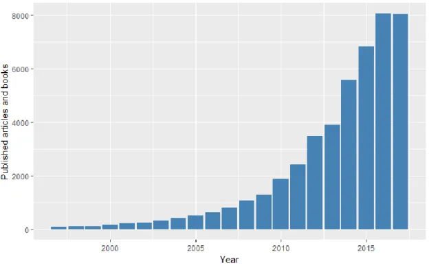
Sports analytics have been a growing field with increased academic and professional relevance. Not only has its use increased in sports organizations, but the number of published articles and books about this topic has grown exponentially. Figure 1 reveals the expanded evolution of sports analytics published articles on Google Scholar over the last 20 years. From a negligible research interest in 1997, we see its continued escalation until the year 2017.

Figure 1 - Published articles and books with keyword “Sports Analytics” from 1997 to 2017 in Google Scholar.

The use of analytics has not only risen in academic research but most importantly, it has sparked interest in most sports organizations and fundamentally changed the way the sports are played (Ofoghi et al., 2013).

It’s being applied throughout many different areas in a sports organization: from scouting and talent identification (Bhandari et al., 1997; Coles, 2015;), to video analysis (Schumaker et al., 2010), to forecasting results (Rotshtein, Posner, & Rakityanskaya, 2005), statistical simulations (Kelley, Mureika, & Phillips, 2006), defining player ratings (McHale, Scarf, & Folker, 2012), performance analysis (Ofoghi et al., 2013), among others.

Currently, most of the discussion about sports analytics either concerns the performance analysis of players or teams or is indirectly related to injury prevention in players (Casals & Finch, 2016). Both require high-quality data, presented with robust statistical approaches.

5 Despite most football injuries being traumatic (Dvorak & Junge, 2000) - hence, not able to be predicted using this methodology), around one-third of all injuries are muscular and so liable to risk factors that contribute to their occurrence (Ekstrand, Hägglund, & Waldén, 2011).The problem of injury prediction has more commonly been studied by identifying these risk factors using typical statistical tools like logistic regression (Bittencourt et al., 2016). This methodology is used to identify linear relationships, but it has its limitations since injuries are a complex phenomenon and it’s not easy to test variables with different weights and feedback loops as well as testing the different causal relationships (Quatman, Quatman, & Hewett, 2009). In the face of multiple factors possibly associated with injuries, it is also necessary to have control of confounding and multiple influences and knowledge.

One of the methods of monitoring different training factors in professional football is the use of sensor data with GPS technology (Aughey, 2011). It allows quantifying with precision the player’s training load by measuring running distances, accelerations, impacts, among others. The use of this data for injury prediction is not yet fully explored (Colby et al., 2014).

Due to the big amount of data produced by these various tracking devices and the multifactorial complex and the dynamic nature of sports injuries, machine learning algorithms and data mining methodology are a particularly good fit. Machine learning in sports injuries has been used for diagnosing, where Bayesian classifiers and decision trees are a common approach for decision making support in the medical field. A number of methods for the diagnosis of sport injuries in football using machine learning have been developed and applied (I. Zelic, Kononenko, Lavrac, & Vuga, 1997) as well as motion capture analysis and assessment for injury prevention (Alderson, 2015) but machine learning models that can enable the identification of the risk factors of injury using training data are not so common in academic publications (Bittencourt et al., 2016) and are only now emerging in recent sports analytics conferences. One possible factor for the scarcity of research is the confidentiality of the data for each team since it can be considered a source of competitive advantage.

A relevant article presented in one of the most well-known sports analytics conferences: MIT Sloan Sports Analytics Conference, proposed to prevent the in-game injuries for NBA players using machine learning (Talukder et al., 2016). The authors have used game data, player workload, and data, and team schedules from two seasons with a sliding window approach where they aggregate the average data for a 14-day span and have a 7-day prediction window for the response variable of whether a player got injured. It’s unlikely that the data of one training session can achieve accurate results, hence this aggregated approach. The results demonstrated strong accuracy in predicting whether a player would get injured in that 7-day prediction window.

6 In football, Kampakis (2016)used machine learning algorithms to attempt to predict injury, uniquely based on sensor data of training sessions of Tottenham Hotspur Football Club. The aggregation window approach was also used with the time frame of a week with promisingresults. It also compares using data only from injured players and using data from all players (injured and non-injured). The study verified that sensor training data could contain valuable information for the task of injury prediction.

Besides objective sensor data, the subjective player self-assessment tools, like Hooper’s Index (Hooper & Mackinnon, 1995) or RPE (Haddad, Padulo, & Chamari, 2014), are also identified as useful tools for monitoring overtraining, quantifying exercise intensity and evaluating individual need for recovery, hence providing valuable information for the task of injury prediction (Kellmann, 2010; Simjanovic et al., 2009).

Considering current academic research has not yet developed a machine learning model with the combination of the training sensor data and the subjective player self-ratings, the present project can amplify previous research by applying different machine learning algorithms using a data mining approach to create a predictive model for football injuries using not only the training sensor data but also the player’s self-rating recovery assessment, which will enrich the available academic literature for injury prediction.

7

3. METHODS AND DATA

3.1.

M

A Data Mining (DM) approach will be conducted to analyze the data and create the injury prediction model. DM is a branch of computer science and artificial intelligence used for the discovery of hidden trends and patterns, as well as extracting knowledge from data sources (Witten, Frank, & Hall, 2011). In business setting, DM is frequently used to obtain new knowledge for decision making, but it can also be used to investigate and explore sports data, particularly elite football performance data (Schumaker et al., 2010). The most frequently used DM techniques are: classification, rule mining, clustering and relationship modeling (Ofoghi et al., 2013).

Data Mining projects don’t have a standard framework to be used in its projects. Nevertheless, the

Cross-Industry Standard Process for Data Mining (CRISP-DM) is a popular methodology frequently used in DM projects to increase their success (Chapman et al., 2000). Even though CRISP-DM was created for business use, the general framework can be easily adapted to a sports data mining project. It outlines a cycle with six phases (Figure 2):

8 In this project, the 6 phases will be composed of the following activities:

1. Business understanding – The first phase aims to define the project objectives as well as the

requirements – done in Chapter 1. Considering this project is to be implemented on a specific football team, this phase was accomplished in collaboration with the team’s objectives. Afterward, this understanding was converted into a data mining problem.

2. Data understanding – This second stage starts with the data collection, organization, and

proceeds with EDA. The organization provides a large quantity of data from training sessions and matches, mostly GPS tracker data and self-evaluation questionnaires. An initial EDA will be able to discover insights in the data, identify data quality problems and discern relevant relationships between variables.

3. Data preparation – This third stage has the objective to use the raw data to construct the final

dataset that is going to be used for modeling. Specific activities done at this phase can be fixing multiple data quality problems and variable transformations to maximize the amount of knowledge that can be extracted from this dataset considering our objective.

4. Modeling – At the fourth stage, different DM techniques are selected, applied and optimized.

Different machine learning algorithms are going to be tested at this phase: Support Vector Machine, Random Forest, Extreme Gradient Boosting, Logistic Regression, among others.

5. Evaluation – At the fifth stage, the constructed model(s) are systematically assessed and

compared to make sure they achieve the objectives defined in the first stage.

6. Deployment – The final stage aims to organize and present the knowledge in a way that can

be used by the organization. The newly obtained knowledge is not useful if the team cannot use it. The IT department of the organization is responsable for the deployment and implementation phase.

9

3.2. S

U

We implement the machine learning models using the scripting language R (R Development Core Team, 2011) along with the Integrated Development Environment (IDE) R-Studio (RStudio team & RStudio, 2015). As an open-source statistical programming language, most of the machine learning algorithms are already implemented in R so that it can be used efficiently in this project.

The libraries used in this project were: “dplyr” (Wickham, Francois, Henry, & Müller, 2017), “VIM” (Kowarik & Templ, 2016) , “ggplot2” (Wickham, 2009), “corrplot” (Wei & Simko, 2017), “psych” (Revelle, 2017), caret (Jed Wing et al., 2017), “ROSE” (Lunardon, Menardi, & Torelli, 2014), “xgboost” (Chen & Guestrin, 2016).

3.3. S

D

D

The data used in this project was collected over the course of one football season by a professional football team. The team collected the training session data of individual players using an Electronic Performance and Tracking System (EPTS). This system uses a device to track player positions using GPS in combination with microelectromechanical devices (accelerometer, gyroscope, digital compass) as well as heart-rate monitors and other devices to measure load and other physiological parameters. Apart from the tracking system, the team also collected self-rating data from the players before and after the training session to monitor self-perceived levels of fatigue and training load.

The original data used for this project was divided into four groups: identification data of each training session (8 variables), training sensor data (16 variables), self-ratings of fatigue, stress, muscle soreness and sleep (5 variables) and injury variables (7 variables) to a total of 36 variables. All the data refers to training sessions during the collected football season.

3.3.1. Identification Data

The training sessions are scheduled using a system of periodization that plans according to appropriate cycles and training phases in a way to prioritize objectives, thus creating precise features for each training session.

This data uses two different cycles: mesocycles and microcycles. The cycles vary in the amount of time. A mesocycle has a duration of roughly one month. A microcycle has a duration of 1 week. In general, one mesocycle has approximately 4 to 5 microcycles.

10 Each training day was also identified about the match day. If the match day is labeled MD, the next day after a match is MD+1, the next two days after a match is MD+2 and the previous day after a match is MD-1. It varies from MD+4 to MD-4. This type of identification allows a precise definition of the training load.

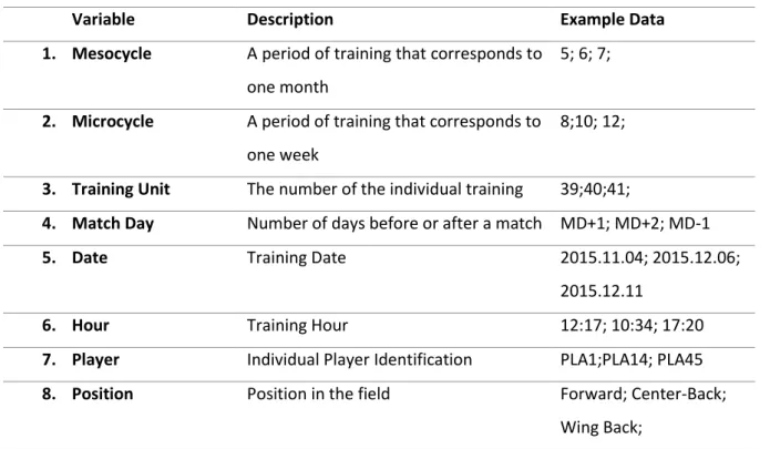
The list of 8 variables in this group described in Table 1.

Table 1 - Identification Variables List

Variable Description Example Data 1. Mesocycle A period of training that corresponds to

one month

5; 6; 7;

2. Microcycle A period of training that corresponds to one week

8;10; 12;

3. Training Unit The number of the individual training 39;40;41;

4. Match Day Number of days before or after a match MD+1; MD+2; MD-1

5. Date Training Date 2015.11.04; 2015.12.06; 2015.12.11

6. Hour Training Hour 12:17; 10:34; 17:20

7. Player Individual Player Identification PLA1;PLA14; PLA45

8. Position Position in the field Forward; Center-Back; Wing Back;

3.3.2. Sensor Training Data

The sensor data of the training sessions was gathered by the EPTS sports tracker StatSports Viper®. This tracker is used by leading teams across the world in multiple sports on top competitions including Premier League, NFL, NBA, among others. The StatSports Viper® streams live data in real-time through the Viper Live Streaming software as well as logging all data for post-session download.

The variables used in this project are not only a result from the GPS data, but they can also be the outcome of a formula using the GPS, accelerometer, gyroscope or magnetometer data provided by the device. All variables are an average of the training session for each player.

11

Table 2 - Training sensor variables list

Variable Description Example Data 1. Training Time Number of minutes the training took 86.67; 112.90;

63.08;

2. Distance Total Total distance covered in a training session 2917.13; 339.43; 2744.56

3. Distance Per Min Total distance covered per minute in a training session

29.65; 32.35; 44.23;

4. High-Speed Running Distance traveled by a player when their speed is in either Zone 5 or 6

7.24;35.32; 63.94;

5. High Speed Running Per Min

Distance traveled by a player when their speed is in either Zone 5 or 6 averaged per minute

1.63; 0.11; 3.00;

6. Heart Rate Exertion Total exertion of a session based on weighted heart rate values

45.13; 18.79; 33.42;

7. Speed Intensity (SI) Measure of total exertion of a player based on “time at speed”

165.73; 279.94; 174.13;

8. Dynamic Stress Load (DSL)

Total weighted impacts 21; 165; 4;

9. Lower Speed Loading Load associated with the low speed (static) activity alone

39.16; 71.76; 8.22;

10. Impacts Number of impacts on a training session 165; 75; 21;

11. Accelerations Acceleration activity on a training session 54; 36; 6;

12. Decelerations Deceleration activity on a training session 45; 16; 27;

13. Sprints Number of sprints in a session 0; 16; 7;

14. Fatigue Index Accumulated DSL from the total session volume. DSL divided by Speed Intensity.

0.56; 0.61; 0.80

15. Energy Expenditure Total energy associated with running (measured in kcal)

311.90;

719.02;660.90;

16. Total Load (TL) Gives the total of the forces on the player over the session

12

3.3.3. Hooper’s Index

The player’s self-ratings were measured with the Hooper‘s Index Questionnaire (Hooper & Mackinnon, 1995), which were filled at the beginning of each training session or game with the goal of measuring the player’s recovery state between training and competitions, as well as to monitor overtraining. Each player answers four items on a 7-point scale where one is “Very, very low” and seven is “Very, very high”. The summation of these four ratings is the Hooper’s Index.

There is a total of 5 variables described in Table 3.

Table 3 - Hooper’s Index variable list

Variable Description Example Data 1. Q1 Item 1: Muscle Pain in inferior members (1-7 scale) 4; 2; 7;

2. Q2 Item 2: Sleep quality of last night (1-7 scale) 3; 2; 4;

3. Q3 Item 3: Fatigue Level (1-7 scale) 5; 7; 3;

4. Q4 Item 4: Stress Level (1-7 scale) 1; 4; 6;

5. SUM Hooper’s Index (Sum of the 4 items) 16; 12; 19;

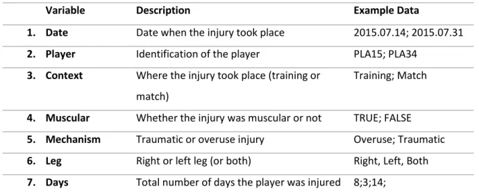
3.3.4. Injury Data

Injury data were manually collected by the coaches as the players got injured during the season into a table. The injuries were differentiated between overuse/muscular and traumatic injuries.

There is a total of 36 rows and seven variables described in Table 4.

Table 4 – Injury variable list

Variable Description Example Data

1. Date Date when the injury took place 2015.07.14; 2015.07.31

2. Player Identification of the player PLA15; PLA34

3. Context Where the injury took place (training or match)

Training; Match

4. Muscular Whether the injury was muscular or not TRUE; FALSE

5. Mechanism Traumatic or overuse injury Overuse; Traumatic

6. Leg Right or left leg (or both) Right, Left, Both

13

4. DATA UNDERSTANDING

4.1. S

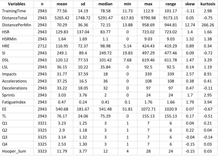
S

Summary statistics of the dataset can be observed in Table 5.

Table 5 – Summary statistics

Variables n mean sd median min max range skew kurtosis

TrainingTime 2943 77.56 14.19 78.58 11.73 112.9 101.17 -1.11 2.98 DistanceTotal 2943 5265.42 1748.72 5291.47 617.83 9790.98 9173.15 0.05 -0.75 DistancePerMin 2943 70.29 36.36 72.15 13.88 958.69 944.81 12.74 266.26 HSR 2943 129.83 137.04 83.77 0 723.02 723.02 1.4 1.66 HSRMin 2943 1.64 1.69 1.1 0 9.03 9.03 1.32 1.38 HRE 2712 116.95 72.37 98.98 5.14 424.43 419.29 0.89 0.34 SI 2943 249.1 89.4 249.72 19.83 497.29 477.46 0.09 -0.72 DSL 2943 120.12 77.53 101.42 7.68 619.46 611.78 1.47 3.29 LSL 2943 36.15 10.22 35.84 0 92.5 92.5 0.14 1.19 Impacts 2943 31.77 37.59 18 0 339 339 2.57 8.91 Accelerations 2943 37.25 16.5 36 0 108 108 0.38 0.41 Decelerations 2943 33.22 18.05 32 0 97 97 0.47 -0.11 Sprints 2943 3.03 3.76 2 0 24 24 1.7 2.95 FatigueIndex 2943 0.47 0.24 0.41 0.1 1.76 1.66 1.79 3.94 EE 2943 540.68 181.67 541.48 51.81 1072.71 1020.9 0.07 -0.67 TL 2943 76.17 24.06 75.29 0 155.13 155.13 0.17 -0.51 Q1 3321 3.23 1.25 3 1 7 6 0.04 0.21 Q2 3325 2.9 1.18 3 1 7 6 0.22 0.04 Q3 3325 3.14 1.32 3 1 7 6 -0.04 -0.14 Q4 3325 2.53 1.30 3 1 7 6 -0.15 0.03 Hooper_Sum 3323 11.79 3.77 12 4 28 24 -0.15 0.03

We can detect a difference on the number of the sensor data variables to Hooper’s variables of approximately 380 observations, which means that in some training sessions where Hooper self-rating was collected, sensor data wasn’t available.

It’s also possible to observe a difference in the scaling of the different variables, the mean values range from 0.47 to 5265.42.

The skewness and kurtosis values indicate that we might have possible outliers on the variables: TrainingTime, DistancePerMin, HSR, HSRMin, HRE, DSL, Impacts, Sprints, and FatigueIndex.

14

4.2. C

M

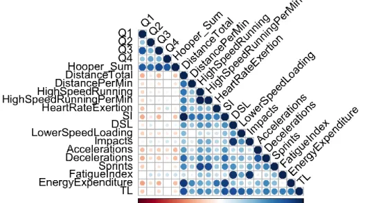
The correlation coefficient measures the extent to which two variables change together and evaluate the monotonic relationship between the different pairs of variables. Spearman rank-order correlation was used to calculate the correlation matrix to uncover the correlation between the different variables to accurately select the machine learning algorithm to apply.

Figure 3 – Correlation plot

Figure 3 presents the correlation plot where – unsurprisingly - it’s possible to observe a strong positive correlation between the Hooper question variables (Q1, Q2, Q3 and Q4) and “Hooper_Sum”. The Hooper variables only have a weak negative correlation with the sensor training data.

Another unsurprising finding is the strong positive correlation of “Sprints” with “High-Speed Running” and “High Speed Running Per Min”, since they measure the same type of activity.

We can also observe the strong positive correlation of “DistanceTotal” with SI (“Speed Intensity”), “Energy Expenditure” and TL (“Total Load”). The longer the distance ran in a training session, usually the higher the training load, this is a predictable discovery.

An interesting finding is a positive correlation of “Impacts” with “Fatigue Index”. A possible interpretation might be that the more fatigued the players are, the more impacts they have. The positive correlation of “Impacts” with DSL (“Dynamic Stress Load”) is only a natural consequence of the DSL formula which is the total of the weighted impacts.

15

4.3. M

V

From Figure 4 we can observe that the variable with more missing values is the Heart Rate Exertion (HRE) with over 32% of the data being missing, which correlates to 1085 observations. Most sensor data variables have approximately 26% missing variables (approximately 1085 observations). The Hooper self-ratings variables have 17% missing records (approximately 707 observations). Considering most machine learning algorithms have difficulties handling missing data, this is a situation that will be handled on the data preparation step.

16

4.4. I

D

On this project, only muscular injuries are used. Muscular injuries can be identified from the training and self-reporting data, unlike traumatic injuries, like the ones originated from a collision during training or a match, which cannot be predicted using this methodology. The injury severity and the time the player was in recovery were not considered for this article.

In 36 total injuries during the season, 18 were muscular injuries. From these 18 injuries, 5 were eliminated for happening outside of the normal season training of the team. The players were injured during the pre-season or during the break for playing with the national team when the training loads are different. Hence, 13 muscular injuries remained. From this observation, it’s possible to conclude that we have an unbalanced dataset.

4.5. V

C

To better understand the dataset and the variable distribution, all the variables were compared with injured observations. This comparison allows recognizing the differences of non-injured to injured players without any machine learning algorithm. The plots were created using the variables with similar scaling for ease of understanding.

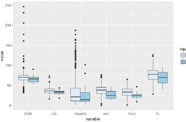
Figure 5 - DistancePerMinute (DPM), LowerSpeedLoading(LSL), Impacts, Accelerations (Acc), Decelerations (Decc) and Total Load (TL) variables splitted between injured and non-injured observations

17 By observing Figure 5, it’s possible to immediately detect that all variables have a slightly lower mean value for the injured observations. On some variables, the difference is considerable higher like for example on Accelerations and Decelerations while other variables have a lower difference: DistancePerMinute (DPM) and LowerSpeedLoading (LSL). Outliers can also be detected on most variables.

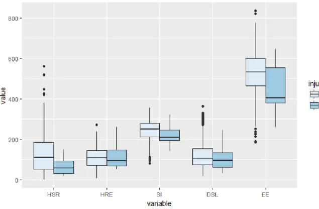
Figure 6 - High Speed Running (HSR), HeartRateExertion (HRE), Speed Intensity (SI), Dynamic Stress Load (DSL), Energy Expenditure (EE) variables split between injured and non-injured observations

Figure 6 shows the effect of injured players having a slightly lower mean on all variables, with some variables having a larger difference like Energy Expenditure (EE), High Speed Running (HSR) and Speed Intensity (SI).

18

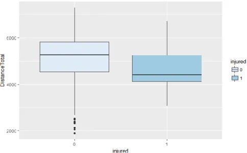
Figure 7 - Distance Total variable splitted between injured and non-injured observations

19

Figure 9 - Fatigue Index variable splitted between injured and non-injured observations

On the remaining three sensor data variables (Figure 7, Figure 8, Figure 9), it’s possible to detect the same scenario of the variables having a slightly lower mean on injured observations. It’s particularly surprising to observe Fatigue Index (Figure 9) where we might expect a higher mean on injured observations than on non-injured.

20

Figure 11 - Hooper Sum variable splitted between injured and non-injured observations

On the self-rating Hooper questionnaire (Figure 10, Figure 11), the relationship is reversed. A slightly higher mean on injured observations can be observed. This is not an unexpected outcome considering higher values of this scale can indicate an imbalance between stress and recovery.

21

5. DATA PREPARATION

5.1. D

P

-P

Previous injury prediction models used aggregated data over a sliding window of time (chapter 2). The reason is that a muscular injury caused by overtraining is typically the result of a sequence of increase in training load and not of one individual training (Kellmann, 2010). Therefore, the model will be more likely to notice the difference in the data that leads to an injury if it’s aggregated data from more than one training.

Considering it wouldn’t be the most efficient approach to use the data of each training individually to predict the injury the data of one microcycle (one week) is, instead, averaged per player. Consequently, each observation is the average of the sensor data and self-ratings of one player in the training units contained within one microcycle. There are at least two training units aggregated for each player. A binary variable [0, 1] indicates whether the player became afflicted by an injury that week or not. Other aggregation windows could have been used (for example: 2 days, 3 days, etc). We considered one week since it usually contains different training intensities and one match, as well as being a frequently used measure in football. Thus, using this window we can collect a more useful range of high-quality data and get a more accurate representation of the player’s recovery and muscular state. Observations that contained missing values were removed during this aggregation process. It could be argued that information is lost by deleting missing values instead of imputing them, but considering this is an unbalanced dataset, imputing them would only further add to the imbalance, as well as add more noise to the data. The methods for correcting the unbalanced dataset already add some noise – taking into account the artificial data methodology (see subsection 5.5.) –, hence the decision to delete the missing values.

Commonly, outliers are deleted (or treated) for better algorithmic performance, but on this dataset, even though outliers are present, it was decided not to delete them due to also deleting observations that belonged to the target injured class. Considering the already reduced number of injured observations, deleting them further would not aid the task of creating a prediction model.

22

5.2. F

S

The variable “Hooper_Sum” was removed considering the variable is nothing more than the sum of the four questions (Q1, Q2, Q3 and Q4), consequently doesn’t add any value to the dataset. The variable “Training Time” was also deleted since it could be misrepresented as an injured player at the beginning of any training will necessarily have a lower training time.

On Table 6is presented the complete list of variables used for the model with example data.

Table 6 - Complete list of variables and example data

Variables Example data

Q1 3.33; 5; 2.75; 2.5; 1; Q2 4; 4; 3.5; 3.5; 2; Q3 3.33; 4.67; 4; 2.75; 1; Q4 3; 4; 3; 2.25; 1; DistancePerMin 69.8; 71.4; 65.4; 64; 58.5; HighSpeedRunning 220.8; 305.8; 276.5; 132.6; 27.4; HighSpeedRunningPerMin 2.64; 3.35; 3.11; 1.41; 0.3; HeartRateExertion 135.3; 164.4; 196; 161.2; 69.1; SI 287; 322; 275; 257; 244; DSL 168.6; 135.2; 205.9; 151.5; 75.1; LowerSpeedLoading 35.2; 35.3; 38.2; 32.1; 34.5; Impacts 43.8; 38; 75.8; 21.3; 13.5; Accelerations 41; 46.8; 45.5; 29.7; 36; Decelerations 41.8; 42.8; 55.2; 36; 24; Sprints 6; 6.25; 5.75; 0.67; 0; FatigueIndex 0.57; 0.41; 0.7; 0.56; 0.32; EnergyExpenditure 621; 608; 614; 506; 587; TL 88.2; 87.8; 84.3; 79.5; 68.9; injured 0; 0; 0; 0; 1;

5.3. T

T

D

A cornerstone of the supervised learning algorithms is the division of data into a training and a testing dataset. The training dataset is used to build the classification model, and the testing dataset serves as the unknown data we wish to predict. 70% of the data is assigned to the training set and 30% to the testing set. The actual number of instances can be seen in Table 7.

This division on an already reduced dataset may raise some questions. If all examples are used in the training process, even if an evaluation technique like cross-validation is used, the algorithm can be optimistic compared to the performance of completely unseen samples. By doing this division, even

23 though we are reducing the number of target variable observations, we gain in the reliability of the results.

Table 7 - Training and testing datasets number of observations

Dataset Partition Total Observations (N) Not Injured (0) Injured (1)

Training 489 479 10

Testing 207 204 3

5.4. B

D

As discussed in Chapter 4 and as it can be observed from Figure 12, the target variable has a highly unbalanced distribution with only 1.9% of the observations of our dataset belonging to injured players.

Figure 12 - Target Variable Distribution Plot

An unbalanced dataset with one prevailing class occurs in many different fields and circumstances. Most commonly, it is found in fraud detection where typically fraud transactions are a rare occurrence on a dataset. It can also be found in social sciences where the researchers might be attempting to identify anomalous behaviors. In these situations, the intrinsic nature of the problem generates an unbalanced dataset. Injuries in football are one of these circumstances where the number of training sessions during a whole season will typically be much larger than the number of injuries.

24 The problem of using an unbalanced dataset in machine learning is the tendency of the model to ignore the smaller class and focus on the dominant class, creating a skewed prediction (Menardi & Torelli, 2014). Hence, overlooking the issue of an unbalanced dataset leads to significant costs, both in model estimation and when the evaluation of the accuracy of the estimated model has to be measured (Batista, Prati, & Monard, 2004).

There are several methods for correcting the problem of the unbalanced dataset. Most research focuses on model estimation stage (Menardi & Torelli, 2014) and uses various techniques of data resampling (such as random oversampling or undersampling) as well the generation of artificial data (using specific algorithms to generate artificial examples similar to the rare observations) (Kotsiantis, Kanellopoulos, & Pintelas, 2006).

For this article, five different data resampling techniques were used as an attempt to correct the unbalanced dataset:

1) Random oversampling: this method randomly replicates N samples from the minority class. The dataset can then become prone to overfitting since the new data is an exact copy of the data of the minority class (Menardi & Torelli, 2014).

2) Random undersampling: this method randomly eliminates N samples from the majority class as an attempt to balance the dataset. The most important problem is the elimination of potentially useful data for the training of the model (Menardi & Torelli, 2014).

3) Random undersampling and oversampling combined: the unified use of undersampling and oversampling with different over/undersampling rates was used with good results in previous studies (Kotsiantis et al., 2006).

4) Synthetic Minority Over-Sampling Technique (SMOTE): is an algorithm that aims to generate artificial examples of the minority class by interpolating between several examples that lie together. This way, it avoids the problem of overfitting that is present in oversampling (Chawla, Bowyer, Hall, & Kegelmeyer, 2002)

5) ROSE: is an algorithm that generates new (artificial) data around the minority class according to a smoothed bootstrap method. Fundamentally, it generates a new synthetic dataset where the two classes have approximately the same number of examples (Menardi & Torelli, 2014). To evaluate the effectiveness of the different data correction methods, they were applied uniquely to the training set, generating five different training sets, each with one different data resampling technique, leaving the testing dataset untouched and unbalanced. The new dataset sizes and the

25 percentage of the injured classes are presented in Table 8. The R code for the dataset division with the different balancing methods is in Appendix 1.

Table 8 – Balanced datasets

Data Correction Method Total (N) Not Injured (0) Injured (1) Percentage of Injured Class Random Oversampling 750 479 271 36%

Random Undersampling 160 150 10 6%

Random Oversampling & Undersampling Combined

410 220 190 46%

ROSE 489 262 227 46%

SMOTE 640 480 160 25%

It can be argued that creating the resampled training dataset with these methods before model fitting may lead to optimistic estimates of performance since they may not reproduce the class imbalance that future predictions would most likely encounter. An alternative solution is to use the resampling during the cross-validation procedure (Kuhn, 2017). But considering the substantial increase in computing time and the decreased level of control of the training set, only the first approach was used.

5.5. R

R

As an attempt to reduce redundancy in the dataset and improve training accuracy, Principal Component Analysis (PCA) was applied to the unbalanced (original) and the five balanced datasets. By reducing the number of features, using PCA, the original dataset is projected into a smaller space by using the k orthogonal non-correlated vectors to represent the data, resulting in dimensionality reduction (Agarwal, 2013). This way dimensionality reduction can be performed on the datasets, and then fit a machine learning algorithm to a smaller set of variables, while maintaining a big part of the variability of the original dataset (James, Witten, Hastie, & Tibshirani, 2013). One of the drawbacks of using this technique is the interpretability, especially after having used the components in a machine learning algorithm. Considering each principal component is a linear combination of the original variables, knowing which variable influenced more the target variable can be hard to explain (Bishop, 2007).

PCA always generates as many components as existing variables (Agarwal, 2013), to select how many of them to retain, there are three well-known heuristic methods (Berge & Kiers, 1996):

26 1) Pearson criterion – or cumulative proportion of explained variance: This criterion recommends retaining the components that explain approximately 80% to 90% of the total variance (Pearson, 1901).

2) Kaiser’s Rule: this criterion recommends retaining as many components as are the eigenvalues larger than 1 (Kaiser, 1960).

3) Scree Plot: This graphical criterion where the curve of the scree plot is used to select the components (Cattell, 1966).

Considering Pearson’s criterion is a popular and elegant method to PCA (Berge & Kiers, 1996) it was the chosen criterion in this project. The cumulative variance of the components on the different datasets can be seen in Table 9.

Table 9 - Cumulative percentage of variance on the six datasets. Emphasis added to the selected number of components.

Components Unbalanced SMOTE ROSE Over Under Both comp 1 37.01 38.33 28.08 39.64 36.49 39.92 comp 2 55.19 56.46 41.62 57.56 54.85 57.84 comp 3 66.16 67.71 52.30 69.09 66.32 70.57 comp 4 73.83 75.31 59.13 76.70 74.41 77.82 comp 5 80.50 81.20 65.03 82.92 81.66 84.37 comp 6 85.13 85.64 69.78 87.08 86.85 88.14 comp 7 88.55 89.21 73.61 90.36 90.57 91.23 comp 8 91.46 92.14 76.88 92.93 93.17 93.58 comp 9 93.96 94.60 80.01 95.20 95.29 95.49 comp 10 95.99 96.47 82.96 96.60 96.70 96.77 comp 11 97.12 97.48 85.59 97.56 97.73 97.84 comp 12 98.09 98.38 87.98 98.49 98.43 98.72 comp 13 98.99 99.15 90.29 99.17 99.02 99.29 comp 14 99.52 99.57 92.46 99.60 99.56 99.66 comp 15 99.77 99.78 94.52 99.80 99.79 99.81 comp 16 99.87 99.88 96.51 99.89 99.89 99.92 comp 17 99.94 99.96 98.30 99.96 99.95 99.97 comp 18 100 100 100 100 100 100

27

6.

MODELING & EVALUATION

6.1. M

S

Different types of models were used to find the most suitable one for the dataset used. Considering the small dataset size, different models can be tested without an exaggerated increase of computing time. Hence six different models were selected based on its characteristics of being able to handle the limitations present in our dataset.

6.1.1. Naïve Bayes

Naïve Bayes has been proven effective in many practical applications, including systems performance and medical diagnosis (Rish, 2001). Despite its shortcoming and even if its probability estimates are not accurate, it can work unexpectedly well in classification (Hilden, 1984), in fact, it has been used as a classifier to support the diagnostic of sports injuries using medical data (Igor Zelic, Kononenko, Lavra, & Vuga, 1997).

6.1.2. Linear Discriminant Analysis (LDA)

Linear Discriminant Analysis, originally proposed by Fisher (Fisher, 1936), has a similar approach to PCA, but not only does it find the component axes that maximize the variance, but it also uncovers the axes that maximize the separation between the projected means of the classes, hence, it can be used for supervised and unsupervised learning (Izenman, 2013). LDA was chosen by its ability to accurately work on smaller datasets in many research areas, not limited to cancer classification, facial recognition, and text classification (Sharma & Paliwal, 2015).

6.1.3. Support Vector Machines (SVM)

SVM is a classification machine learning algorithm that uses a maximization of the margin between two classes closest points to seek the optimal separating hyperplane between these two groups (Cortes & Vapnik, 1995). When a linear separator can’t be found, observations are projected through kernel techniques, into a higher-dimensional space where they become linearly separable (Shmilovici, 2010). Even though SVM has been successfully used in a whole range of applications, it tends not to be the best choice when dealing with imbalanced datasets where the positive instances are rare compared to negative ones (Wu & Chang, 2003). However, when used in combination with balancing

28 techniques like oversampling and undersampling, it can improve its effectiveness significantly by making SVM more sensitive to the positive class (Akbani, Kwek, & Japkowicz, 2004), hence making it a useful algorithm for the injury problem.

6.1.4. Artificial Neural Network (ANN)

An ANN uses mathematical models in a way to emulate the interactions of neurons in the brain. It learns from the training data the arbitrary nonlinear input-output connections by automatically adjust layer weights or even the network structure (James et al., 2013). It can be used to solve problems that are not solvable by conventional mathematical processes (Lang, Pitts, Damron, & Rutledge, 1997) There has been an increasing interest in the use of ANNs in different types of domains. ANN have successfully been used in the past to characterize relationships in muscle activity and kinematic patterns (Hahn, 2007), performance modelling in sports (Silva et al., 2007), to predict relationship between perceived exertion and GPS training-load variable (Bartlett, O’Connor, Pitchford, Torres-Ronda, & Robertson, 2011) and a valid tool for modelling the training process (Shestakov, 2000). They can be used to improve our understanding of the relationship between the player injury and the GPS and self-rating features.

6.1.5. Ensemble Models

Two ensemble models were used to reduce bias and variance and overcome the limitations of the small size and unbalanced dataset: Random Forest (bagging) and Extreme Gradient Boosting (Boosting). Ensemble models generate and combine an elevated number of classifiers created on smaller individual subsets of data to produce an (expectantly) better estimator. This combination is made in two ways: bagging (e.g. random forest) and boosting (e.g. XGBoost) (Dietterich, 2000). Bagging (which stands for Bootstrap Aggregating) algorithm randomly partitions the data into subsets (using bootstrap) and trains the base learners, compute the ensemble and use voting or averaging for the classification or regression, respectively (Dietterich, 2000). A boosting algorithm is sequential, instead of generating different classifiers – as bagging -, boosting turns weak learners into strong ones, by focusing on the examples previously misclassified to build the new classifiers (Friedman, 2001). The bagging algorithm used is Random Forest, which uses an ensemble of classification trees (Breiman, 2001). Bootstrap is used to divide the data into subsets, build a classification tree and at, each split, uses a random selection of features. Each tree is grown to its full extent to reduce bias and the

29 ensemble of trees then votes for the most popular class (Pal, 2005). It was chosen to use in this project by its predictive performance, not overfitting and incorporating the interactions among features (Díaz-Uriarte & Alvarez de Andrés, 2006).

The boosting algorithm used is Extreme Gradient Boosting (XGBoost) (Chen & Guestrin, 2016). XGBoost was chosen for being an efficient implementation of the gradient boosting ensemble (Friedman, 2001), its respectable performance on machine learning competitions (Chen & He, 2015) and its reliant use on other domains (Tamayo et al., 2016; Torlay, Perrone-Bertolotti, Thomas, & Baciu, 2017). The boosted trees on XGBoost can be regression or classification-based trees.

6.2. T

C

P

For training control stratified, 4-fold Cross Validation is used. K-fold cross-validation is a resampling technique widely used in model validation (James et al., 2013). On this approach, the observations are drawn without replacement into four groups of approximately equal size and an equal proportion of classes. The first fold is used as a validation set, and the classifier is fitted on the remaining three folds. The excluded group is used as a statistically independent test sample for the model. Each group is excluded once. A smaller k (k=4) was used due to small sample size.

A parameters grid was used for training each model to find the optimal settings. The grid used is designated in Table 10.

Table 10 - Model parameter grid

Model Parameters

Naïve Bayes -

Linear Discriminant Analysis Discriminant Functions ∈ {1,2,3}

Support Vector Machines Cost ∈ {0.25; 0.5; 1; 64}; Sigma ∈ {0.0357}

Neural Networks Size ∈ {1…40}; Decay ∈ {0…0.1}

Random Forest Randomly Selected Predictors ∈ {2…18}

Extreme Gradient Boosting Boosting Iterations ∈ {1…30}; L2 Regularization ∈ {0…2}; L1 Regularization ∈ {1…4}; Learning Rate ∈ {0.01; 0.1…1}

30

6.3. E

The most popular and used evaluation metric to assess the performance of a machine learning algorithm is classifier accuracy (Provost, Fawcett, & Kohavi, 1997) which can be considered as the probability of success in identifying the right class of an observation (Maratea, Petrosino, & Manzo, 2014). However, on an unbalanced dataset where 99% of the observations belong to one class and only 1% to target class, accuracy can easily achieve 99% without correctly classifying any of the target examples. So, the conventional approach can produce misleading results (Weng & Poon, 2008). The other issue with using accuracy as the evaluation metric is the problem with the misclassification costs. Especially on an unbalanced dataset, the target class (rarer examples) is – often – more important than the majority class, so that the cost of misclassing the target class is higher than to misclassify the majority class (Weng & Poon, 2008). In our dataset, misclassifying a muscular injury could have potentially higher adverse effects (as seen in Chapter 1) than misclassifying the majority class. So, we are willing to accept a potentially lower ability to predict the majority class (non-injured), as long as, the classifier accurately predicts the target events (injured players).

Therefore, the measures of recall and precision tend to raise its importance in an unbalanced dataset. In binary classification, it’s possible to outline the observations into two classes: negative and positive, which leads to four possible outcomes: True Negatives, False Negatives, True Positives and False Positives. Different metrics are calculated based on these outcomes.

Precision is also known as Positive Predictive Value, can be considered as a measure of the classifier correctness. A low precision can indicate many false positives. It is calculated using the formula below:

𝑃𝑟𝑒𝑐𝑖𝑠𝑖𝑜𝑛 = 𝑇𝑟𝑢𝑒𝑃𝑜𝑠𝑖𝑡𝑖𝑣𝑒𝑠

𝑇𝑟𝑢𝑒𝑃𝑜𝑠𝑖𝑡𝑖𝑣𝑒𝑠 + 𝐹𝑎𝑙𝑠𝑒𝑃𝑜𝑠𝑖𝑡𝑖𝑣𝑒𝑠

And recall (also known as sensitivity), which can be considered a measure of a classifier thoroughness. A low recall can indicate many false negatives. It’s calculated using the formula below:

𝑅𝑒𝑐𝑎𝑙𝑙 = 𝑇𝑟𝑢𝑒𝑃𝑜𝑠𝑖𝑡𝑖𝑣𝑒𝑠

𝑇𝑟𝑢𝑒𝑃𝑜𝑠𝑖𝑡𝑖𝑣𝑒𝑠 + 𝐹𝑎𝑙𝑠𝑒𝑁𝑒𝑔𝑎𝑡𝑖𝑣𝑒𝑠

These two metrics allow to grasp the relationship between the different classes and to get a more honest evaluation of an unbalanced dataset. A commonly used metric when evaluating unbalanced dataset, which combines recall and precision, is the ROC curve, which plots recall against the False Positive Rate (NOT precision) at various thresholds which allows to directly observe the tradeoff between them (Powers, 2011). The ROC curve, using a dynamic threshold approach, can transmit knowledge about the classifier performance in all possible combinations of the class distributions and

31 the cost misclassification (Drummond & Holte, 2004). However, a possible complication is that, on our unbalanced dataset, the ROC curve can still present an optimistic assessment (Drummond & Holte, 2004) since they decouple the classifier performance from class skewness and the error costs (Fawcett, 2006).

An evaluation measure that can help probe the results of a dataset with a class unbalance is the F-measure (Powers, 2011). The F-F-measure, originated from the field of Information Retrieval, is calculated using the formula below (Provost et al., 1997):

𝐹 − 𝑀𝑒𝑎𝑠𝑢𝑟𝑒 = 𝐹1 = 2 ∗ 𝑝𝑟𝑒𝑐𝑖𝑠𝑖𝑜𝑛 ∗ 𝑟𝑒𝑐𝑎𝑙𝑙 𝑝𝑟𝑒𝑐𝑖𝑠𝑖𝑜𝑛 + 𝑟𝑒𝑐𝑎𝑙𝑙

F-measure is the harmonic mean of precision and recall (Sasaki, 2007). F-measure combines them into a single measure, usually with equal weights on both measures, and is also commonly used on unbalanced datasets (Powers, 2011; Weiss & Hirsh, 2000).

32

7. RESULTS AND DISCUSSION

7.1. R

(W

PCA)

The results of the different models and the different sampling techniques (without PCA) are presented in Table 11 and Figure 13.

Table 11 - Training and testing evaluation measures of the models trained with the different datasets

Balancing Model F-Measure Precision Recall

Training Testing Training Testing Training Testing

None NB 0.11 0.1 0.06 0.56 0.5 0.67 None LDA 0 0 0 0 0 0 None SVM 0 0 0 0 0 0 None NN 0 0 0 0 0 0 None RF 1 0 1 0 1 0 None XGBoost 0 0 0 0 0 0 Over[r1] NB 0.73 0.33 0.61 0.29 0.9 0.67 Over LDA 0.84 0.12 0.78 0.06 0.92 0.67 Over SVM 0.99 0 0.99 0 1 0 Over NN 1 0 1 0 1 0 Over RF 1 0 1 0 1 0 Over XGBoost 1 0 1 0 1 0 Under NB 0.23 0.08 0.14 0.043 0.6 0.67 Under LDA 0.14 0.12 0.25 0.07 0.1 0.33 Under SVM 0 0 0 0 0 0 Under NN 1 0 1 0 1 0 Under RF 1 0 1 0 1 0 Under XGBoost 0.67 0 1 0 0.5 0 Both NB 0.75 0.05 0.65 0.03 0.89 0.67 Both LDA 0.92 0.09 0.86 0.048 1 0.67 Both SVM 1 0 1 0 1 0 Both NN 1 0 1 0 1 0 Both RF 1 0 1 0 1 0 Both XGBoost 1 0.12 1 0.08 1 0.33 SMOTE NB 0.65 0.04 0.53 0.02 0.84 0.33 SMOTE LDA 0.72 0.13 0.69 0.07 0.76 0.67 SMOTE SVM 1 0 1 0 1 0 SMOTE NN 1 0.25 1 0.15 1 0.67 SMOTE RF 1 0 1 0 1 0 SMOTE XGBoost 1 0.15 1 0.1 1 0.33 ROSE NB 0.75 0.05 0.69 0.028 0.82 0.67 ROSE LDA 0.72 0.08 0.70 0.044 0.74 0.67 ROSE SVM 0.97 0.1 0.96 0.056 0.98 0.67 ROSE NN 1 0.1 1 0.05 1 0.67 ROSE RF 1 0.08 1 0.042 1 0.67 ROSE XGBoost 0.50 0.40 0.44 0.29 0.59 0.67

33 Figure 13 – Plot with F-Measure of the testing dataset (without PCA)

From Table 11, we can detect several results of overfitting to the data particularly on the more complex models like NN and RF where the F-Measure, Precision, and Recall often have the value of 1 on the training set - a perfect fit - yet, on the test set, the results are considerably worse.

It’s also possible to observe that the training set without any balancing technique has the worst results with most of the algorithms not being able to make any accurate predictions on the testing dataset. The training sets where we applied algorithms that generate artificial data (SMOTE and ROSE) generally have better results.

It’s particularly interesting to detect that a “simpler” algorithm like Naïve Bayes and LDA, often outperform the more complex ones, like NN, RF, and XGBoost in the F-Measure testing set. Such is the case on the no balancing, over and under balancing. Particularly Naïve Bayes has the second highest performance on all the datasets with an F-Measure of 0.33 on the underbalanced testing dataset as we can notice in Figure 13.

The overall problem of most of the used algorithms is in the precision results. The recall achieves a maximum of 0.67 on other ML algorithms, but it’s usually at the cost of a lower precision result. So, in

34 general, the algorithms tend to have little discriminatory value since they have too many false positives.

The best result in this table is with the ROSE balancing technique and the XGBoost algorithm (eta=0.2;

lambda=0.2; alpha=4; nrounds=20)with an F-Measure on the testing dataset of 0.4. This result stands

out due to the increased precision (0.29) since the recall (0.67) can also be found on the other algorithms. On this dataset, the ROSE balancing technique outperforms most of the other balancing techniques.

7.2. R

(W

PCA)

The results with PCA application are presented on Table 12 and Figure 14.

Table 12 - Training and testing evaluation measures of the models trained with the different datasets (with PCA).

Balancing Model F-Measure Precision Recall

Training Testing Training Testing Training Testing

None NB 0.11 0.1 0.06 0.05 0.5 0.67 None LDA 0 0 0 0 0 0 None SVM 0 0 0 0 0 0 None NN 0 0 0 0 0 0 None RF 1 0 1 0 1 0 None XGBoost 0 0 0 0 0 0 Over NB 0.71 0.06 0.61 0.03 0.86 0.67 Over LDA 0.1 0 0.06 0 0.4 0 Over SVM 0.12 0 0.07 0 0.4 0 Over NN 0.18 0.06 0.1 0.03 0.9 0.33 Over RF 1 0 1 0 1 0 Over XGBoost 1 0 1 0 1 0 Under NB 0.23 0.08 0.14 0.04 0.6 0.67 Under LDA 0 0 0 0 0 0 Under SVM 0 0 0 0 0 0 Under NN 0 0 0 0 0 0 Under RF 1 0 1 0 1 0 Under XGBoost 0 0 0 0 0 0 Both NB 0.75 0.05 0.65 0.02 0.89 0.67 Both LDA 0.07 0.04 0.04 0.02 0.5 0.33 Both SVM 0.09 0.04 0.05 0.02 0.5 0.33 Both NN 0.15 0.08 0.08 0.04 1 0.67 Both RF 1 0 1 0 1 0 Both XGBoost 0.98 0.11 0.96 0.06 1 0.33 SMOTE NB 0.65 0.04 0.53 0.02 0.84 0.33 SMOTE LDA 0.07 0 0.05 0 0.1 0 SMOTE SVM 0 0 0 0 0 0 SMOTE NN 0 0 0 0 0 0

35 SMOTE RF 1 0 1 0 1 0 SMOTE XGBoost 0.55 0 0.75 0 0.43 0 ROSE NB 0.75 0.05 0.69 0.03 0.82 0.67 ROSE LDA 0.08 0.04 0.04 0.02 0.6 0.33 ROSE SVM 0.09 0.04 0.05 0.02 0.5 0.33 ROSE NN 0.09 0.04 0.05 0.02 0.5 0.33 ROSE RF 1 0.08 1 0.04 1 0.67 ROSE XGBoost 0.5 0.22 0.72 0.13 0.38 0.67

Figure 14 - Plot with F-Measure of the testing dataset (with PCA)

From Table 12, it’s possible to notice overall worse results with the application of PCA on the different datasets.

The patterns detected on Table 11, can also be observed here. The dataset with no balancing technique can’t generate any predictions (except for Naïve Bayes). NN and RF often overfit with training values of 1 and worse values on the testing dataset.

It’s particularly interesting to note that the SMOTE balancing technique only has prediction with Naïve Bayes, not generating any predictions with the other algorithms. Since both ROSE and SMOTE generate artificial data, we would expect better values on both.