A Work Project, presented as part of the requirements of the Award of a Master’s Degree in Economics from the Nova School of Business and Economics
PORTUGUESE STAGNATION IN THE 2001-2012 PERIOD
MANUEL FRANCISCO CALDEIRA DO VALE DA COSTA REIS 21123
A Project carried out under the supervision of Professor Luís Campos e Cunha
Page 2 of 25 Abstract
The 2001-2012 period has been one of very low growth for Portugal. This work project tries to find reasons for this slowdown. Growth in real GDP will be explained by several variables ranging from education, capital, government and world markets. Compensation of employees, capital per worker and the exports of competitors seem to explain a significant part of the slowdown. The ratio of non-tradables to tradables is also included but not significant, maybe due to a poor sample size. Stagnation then seems to be caused both by low growth in input accumulation and productivity as predicted by Amador and Coimbra in 2007.
Page 3 of 25
I. Introduction
Stagnation is a problem largely forgotten about in the developed world. A period of sustained lack of growth implies a loss of economic power comparatively to most other countries. During the 2001-2012 period Portugal grew 0.1% and, alongside Italy, was the least growing country in the European Union. The average growth for the union was of 1.3% and of 1.0% for the Euro Zone. This work project aims at exploring what were the reasons for the low growth Portugal had during this period. The explanations will be rooted in economic theory and several papers on stagnations.
This decade had a lot of major world events influencing the economy. Two major stock market crashes and a bubble in between them. The introduction of the Euro and the rise of China are some of the factors that permeated the time period. Some of them were particularly hard hitting for Portugal. The Euro removed the ability to have a managed currency which ensured competitive exports. On the flip side it helped stabilize inflation, currency rates, and interest rates possibilitating cheaper external debt. Entry in the European Monetary Mechanism also changed the banking system of EU countries by forcing European wide rules and restrictions. Adding to that the 00s were a period of great growth for China, Korea, and the Eastern European countries as they entered the world exports market. This created new avenues for foreign direct investment and better deals for investment in low-wage environments. This period also had a great boom for commodity prices most representatively in oil and food prices.
The paper is divided 4 major parts. First a literary review that will look at both papers on lost decades and economic growth in general. Second, the variable choices and
Page 4 of 25 sources will be presented. Third, the model will be presented and finally the estimation results discussed.
II. Literary Review
a) Stagnations
Stagnations are normally caused by some underlying issues in the economy. The Japanese case is the most well-known as the fastest growing economy between 1960 and 1980 suddenly stopped. The thesis normally presented for Japan is that there was a breakdown of the financial system leading to decreased investment gains. However
Hayashi and Prescott (2001) show another possible explanation: that a generalized decrease in total factor productivity growth is to blame for the prolonged stagnation. In fact they attribute the bubble to the predicted future productivity growth which never happened. They state that the decrease in productivity stems from an exogenous decline in technology. Kawamoto (2004) analyses this thesis by creating a better estimate of technological growth. What he finds is that technology did not slow down. The productivity slowdown is then not due to a lacking technological progress but instead to other factors affecting productivity namely “increasing returns, imperfect competition, cyclical utilization of labor and capital, and reallocation effects.”
A paper by Bergoeing et al. (2002) explores the differences in growth between Mexico and Chile in the 80s. Both countries withstood a recession followed by stagnation. Chile had a much quicker recovery. Typical explanations for this difference range from the better monetary policy of Chile, the faster decline in real wages that fueled exports and
Page 5 of 25 Mexico’s debt overhang. What Bergoeing et al. find is that Chile had better government policy in general which allowed for productivity gains. Market liberalization, Law changes, and financial system changes improved productivity and made sure that zombie firms stopped existing, opening up the market.
Ricardo Reis wrote in 2013 a paper exploring the Portuguese case. Most facts associated with Portuguese low productivity did not suddenly change in the turn of the century and, according to Reis, cannot be the answer. Low education, increasing
government size, a rigid labor market among a number of other issues are not the focus of his paper as they did not change much during this period. He argues that entry in
international capital markets with an underdeveloped financial system created wrong incentives for investments which lowered productivity. As such, the large capital inflows associated with the entry in the Euro Zone incentivized banks to lend indiscriminately allowing inefficient firms to remain in operation. There was also a much larger investment in non-tradables which further increased the costs facing exports.
Amador and Coimbra (2007) paint a different picture. They argue that what is lacking in Portuguese GDP growth, comparatively to Spain, Greece and Ireland, is that Portuguese growth is mostly reliant on input accumulation due to a low productivity rate. This is because of a lower capital-labor ratio and low-technology industries. Both papers agree that there are long-term issues in the Portuguese economic structure, the difference of opinion arises in whether or not they are to blame for the stagnation. Reis believes they aren’t and that it must be a new factor that appeared in the 00s namely the increase in
Page 6 of 25 capital inflows and the over-investment in non-tradables. Amador and Coimbra state that the issue was low productivity and a stop in the accumulation of inputs.
Finally Olivier Blanchard (2006) paints a grim picture of the Portuguese reality. He tries to lay down some possibilities for future policies which can be either through increases in productivity or decreases in input prices. He states that the reasons for the slump arise from the over optimistic evaluation of the economy in the 90s. The entry in the European Monetary Union raised hopes in investors for faster growth. Investment and Consumption increased by trimming off savings. Once again the structural issues of low productivity weigh heavily on growth and when input accumulation stopped (due to the excessive accumulation in the 90s) the results was not good.
The general idea that is extracted from these papers is that productivity is king. Most of these cases of stagnation highlight that the relationship between inputs and outputs is the most important factor determining growth. The Portuguese case, seems to follow this. Portugal did not have a very strong productivity growth historically and as soon as it
stopped accumulating inputs growth stopped.
But what influences Total Factor Productivity? According to a 2007 U.N. Industrial Development organization working paper there are many factors that affect TFP. Some examples are capital intensity, education, technology, institutions, health, among many others. The main conclusion from this extensive literature review is that most of the analytical links between TFP and variables are determined empirically and, according to the paper, is that it is “yet too inconclusive for policy implications.” Essentially there is no
Page 7 of 25 consensus on the true cause but capital intensity, education, technology and institutions seem very likely candidates.
b) Growth
Growth theory provides the theoretical framework that helps explain how the inner workings of an economy help it grow. The starting point is the Solow growth model generally seen as the solid base for further extensions. It states that the main factors that cause growth are capital accumulation, labor and total factor productivity. Lucas (1988) provides extensions for this model by introducing factors such as technological change and human capital accumulation through learning by doing and schooling. Portugal has a traditionally poor schooling system which still has not covered many parts of the
population. Even though it is improving its effects are still not generalized as there is still a lot of the population without any education besides the first four years of schooling.
Learning by doing could be a source of human capital accumulation in Portugal but it is somewhat hard to measure on a macro level. This paper also mentions the benefits of international trade to GDP growth. The two previous papers provide a strong basis for variables including both the stock of labor and capital. As such Capital per worker, per hour and per educated person will be used.
As evidenced from the previous section the increase in foreign capital has been a determining factor in recent years. However its role on growth can be dubious. E. Borensztein et al. (1998) present the idea that FDI increases growth given a certain technological level in the country. This means that large foreign investment may become somewhat meaningless if the country cannot accept the technological improvements (in
Page 8 of 25 case the country is lagging behind in technological terms). This may mean that the foreign capital growth was rendered useless due to low human capital. Further down the work project it will be seen if there was a significant impact or not. Another important aspect regarding technology is the ability to increase the production possibilities frontier. Romer (1990) creates a 3-sector model in which human capital can be devoted to research. By allocating some capital to the creating of more technology the country increases
productivity. Human capital is once again a cornerstone for growth and it spills over to productivity growth.
The trade balance was one of the first issues to be studied in economics and its importance has only increased. It is generally accepted that trade improves the welfare of a country as it expands the available market, product selection and prices. Frankel and Romer (1999) show another possible way trade increases income. “Trade appears to raise income by spurring the accumulation of physical and human capital and by increasing output for given levels of capital”.
Finally there is one last factor that is important for Portugal: the Government. Easterly and Rebelo (1993) provide an in-depth look into this matter and find that “the evidence that tax rates matter for growth is disturbingly fragile.” This statement seems to be verified later by the regressions. However public investments, namely in transport and communications, can yield net positive returns. There is still the flipside where public investment yields a lower return than the investment it crowded out yielding a net negative for society.
Page 9 of 25
III. Data
Inspired by the theories presented above a set of variables was selected. The time period used in the model is from 1979 to 2013. Most of the data is from the AMECO database. For the explained variable, real GDP was used; it is the most common replacement for output.
The first candidate for explanatory variable was productivity. Many of the typical variables for productivity cannot be used as they are calculated using GDP. GDP per hour has a similar problem. A surrogate indicator is then needed. Return on capital, the
compensation of employees, or institutional information could provide for a decent substitute for productivity.
Education is highlighted as another important factor. The Barro-Lee dataset which includes the percentage of population that has attended several degrees of education is quite extensive but only has quinquennial data. There is another dataset by the world bank
featuring gross enrollment in either primary, secondary or tertiary school. Even though the time series was long enough there were some breaks. The solution for this was using a linear interpolation to fill in the blanks. The biggest gap is during the 81-85 period where secondary education has a 5-year break. The remaining breaks are only of one period. Even with this makeshift methodology the data seems to have a good fit as increases in
enrollment aren’t particularly great during the missing period. The other side of human capital, learning by doing, is difficult to capture for the economy as a whole, because of this it won’t be included.
Page 10 of 25 Investment is also very important for economic growth. A set of variables was tried. Foreign Direct Investment, loans to households and financial corporations, and net return on net capital. The latter variable has some issues when used conjointly with the
compensation of employees due to its calculation. Regarding return on capital, which is essential to determine the degree of investment, two variables were tried: The interest rate on Portuguese Debt and the return on the Portuguese stock market.
Joining both the education and capital variables is capital intensity. Three types will be calculated because of the various possibilities. The stock of capital, calculated by
AMECO by compiling GFCF for a large number of years, is divided by hours worked in the economy, by workers and by the gross enrollment in secondary education times the population. This yields three variables: Capital per hour worked, Capital per worker and what will be called Effective Capital for simplicity.
Another possible influence on investment is the government size or taxation which could be causing crowding out. A couple of variables that were created in order to capture both education and capital was the stock of capital per worker, per hour worked and per person times the rate of enrollment in secondary education. Unfortunately the breaks in the Barro-Lee dataset make it unusable.
During this time period three important events happened that could have a direct effect in exports: The introduction of the Euro, the entry of many developing countries to the world markets, and the dramatic increases in oil and food prices. The price of crude was obtained from the FRED database, it would be more correct to use Brent but the variation is similar and WTI crude oil had a longer time series. To include the entry of developing
Page 11 of 25 countries an index of competitor countries was created; the process is described below. The differential between growth in exports in competing countries vs. those of Portugal may also be relevant. Calculating this was a multi-step process.
First the revealed advantage was computed from the OECD database on exports by commodities. This list of about 100 commodity types has exports from 35 countries1 which will henceforth be representative of world exports. From this list the revealed comparative advantage for each commodity in each country was calculated. Countries that revealed advantages similar to those of Portugal during the sample of 1989 to 2007 were considered competitors. The list of competitor countries considered is, by decreasing amount of similar industries: Spain, Belgium, Czech Republic, Estonia, Turkey, Italy, Poland, and Austria. The Competitor exports are then a weighted average of these countries exports.
The variables for government intervention are sparse for Portugal. Still, as
government can influence growth, some variables were included. On the revenue side both direct taxes, indirect taxes, deficit and total tax burden were included. On the spending side total government consumption could not be used as is connected to GDP and most other variables had a small sample size. Subsidies were then chosen as an example variable for government spending. Most other interesting variables had too small a sample size, mostly ranging from 1995 to 2013.
1 Australia, Austria, Belgium, Canada, Chile, Chinese Taipei, Czech Republic, Denmark, Estonia, Finland, France, Germany, Greece, Hong Kong, Hungary, Iceland, Ireland, Israel, Italy, Japan, Korea, Luxembourg, Mexico, Netherlands, New Zealand, Norway, Poland, Portugal, Slovak Republic, Slovenia, Spain, Sweden, Switzerland, Turkey, United Kingdom, United States.
Page 12 of 25 Lastly the non-tradable to tradable ratio and the consumer price index growth for construction and dwellings were included. These should be significant if there was a drag caused by over investing in exportless sectors.
IV. Model
The model used in this work project was determined empirically. The final variable list is in table 1. All of the variables were tested on unit roots and many were promptly discarded or transformed. Issues also arose as some the variables available are derived from GDP and are endogenous. Problems with causality also can occur. First, every variable was regressed on GDP in order to provide an initial overview of the interactions. Then several attempts at final regressions were made, each taking into account variables for inputs, productivity and world events. These models were thoroughly tested in regards to
heteroskedacity, serial correlation, multicollinearity, over specification and causality. Table 7 describes the best models that were obtained.
Some variables are clearly better than others. Effective capital seems to be better than capital per worker in all regressions. Capital per hours worked was difficult to use as it had a causality issue with GDP (Did GDP increase because the number of hours increased or vice-versa?) since no instrumenting solution was found for hours it was ignored.
Competitor’s exports growth yields more significance to the model than world exports. Both growth in loans and CPI changes seem to lose significance when used with the other variables. The question then becomes whether to use the growth in real wages, the growth in average nominal wage or the growth of nominal wage per worker. Before making this decision there is still one important issue.
Page 13 of 25 Causality was a major preoccupation as it was unclear whether an increase in GDP would increase compensation or vice-versa. Answering this required experimenting with an Instrumental Variable model in which compensation was considered endogenous. In order to find suitable instruments variables with high correlation with the explanatory variable but low correlation with GDP growth were needed. Table 8 has the correlation for some variables. The resulting IV regressions, in table 9, all seem to have good instruments and the instruments seem to be valid according to the Sargan test. Where there is some
difference is in the Wu-Hausman test which states that the real compensation is exogenous and does not need to be instrumented, this is some evidence that real compensation causes GDP growth and not the other way around. The reason for the inverse causality in nominal compensation could be the influence of GDP growth in increases in the price level. Even if real compensation was endogenous the quality of its model, as measured by r-square, was higher than the others. Real compensation growth was then used for the final model.
𝑌𝑑,𝑡= 𝛽0+ 𝛽1𝑟𝑐𝑒𝑑,𝑡+ 𝛽2𝑒𝑥𝑐𝑜𝑚𝑝𝑑,𝑡+ 𝛽3𝑘𝑙𝑑,𝑡+ 𝛽4𝑌𝑑,𝑡−1 ( 1)
T indicates time and d the yearly percentage change. As such the above model says that the yearly change in real GDP is linearly dependent on the growth in real compensation of employees (rce), the export growth of the main competitors from Portugal, and the growth in the ratio of Capital per capita times the gross enrollment in secondary education.
V. Results
The estimation results are in the table 10. Figures 1 and 2 help visualize the patterns variables took during this period.
Page 14 of 25 Capital per person with secondary education has a positive impact on growth, increasing the amount of capital an educated worker has leads to greater output for the economy. During the 90’s this variable experienced great growth that suddenly stopped in the early 00s and began decreasing. Less inputs will lead to lower growth if there is not a corresponding productivity growth, which there is no evidence of.
The exports of competitors also improves Portuguese GDP. This is most likely because Portuguese exports have little say in global terms and simply follow the trends. It is important to note that competitor’s exports are better at describing GDP than world exports and that around 1998 the difference between growth rates starts being more
noticeable. This could lead to a slowdown in Portuguese exports and as such would explain part of the stagnation of GDP. Another interesting fact is that the difference between Portuguese exports and the competitor’s exports has lessened in the studied period. In the early 90s the difference became close to zero. Before that Portuguese exports consistently grew faster when more competitors started entering the markets the growth rates converged and Portugal lost its edge.
Finally the real compensation of employees. The sign is positive which goes against initial idea that it would decrease productivity by increasing costs. It could in fact be the other way around. Businesses are only increasing wages when the productivity enables them to do so meaning that this variable would actually follow the growth in productive capacity. It could also be an effect from the higher purchasing power that households gained which increases consumption. This is speculation and there are many other possible reasons.
Page 15 of 25 Another important regression includes the growth in the percentage of non-tradables to tradables showed in table 11. This is inspired by the Reis paper in which he attributes a great deal of the crisis on the increase of this ratio. The issue for this variable, and the reason for its exclusion in the main model is that is has a low sample size of only 16 data points. Even so when included in the regressions it did not reach significance. Still, a more through dataset would be needed to make a strong claim on the importance or not of this variable.
What these results tell is that what happened in Portugal is similar to the case of Japan, Mexico and Chile. There was a lot of factor accumulation in the 80s and 90s that suddenly stopped in the turn of the century. The reasons for this drop in factor
accumulation are not entirely clear. What is evident from other time series is that net return on net capital stopped increasing since 1987. The only other country in the AMECO database with a similar situation is Spain. Two other countries also had a decrease in net return during the 1960-2013 period: Greece and Belgium.
Regarding the variables that didn’t make it to the final cut there are some interesting factors. Oil prices seem to be somewhat uncorrelated with the stagnation. Oil should have an impact as it increases both the cost of transportation and electricity. Foreign direct investment is also a notable absence. Initially there was the expectation that FDI would improve growth but, as Borensztein et al. (1998) state, FDI doesn’t necessarily increase growth if there is not a sufficient level of education. As predicted in Easterly and Rebelo (1993) taxation had no significant effect but it proved a good instrument for some variables.
Page 16 of 25 These regressions should be econometrically correct and, although simple, provide some insights on the growth of Portuguese GDP. Labor has an important role as it is the main input in production and its compensation has a positive impact in GDP. Effective capital is very important for growth as it provides labor the means of production. Finally the external sector provides a way of funneling production and for new money to enter the economy.
VI. Conclusion
So what did happen to Portugal? What the above model seems to indicate is that capital intensity and compensation began to stagnate. Export growth, namely in the sectors in which Portugal has a competitive advantage, seems to have also slowed down. The factors allied with momentum in GDP growth made growth slowdown immensely.
Amador and Coimbra (2007) seem to be right when they state that Portugal owes most of its growth to factor accumulation. The comment on Reis (2013) by Olivier Blanchard also seconds’ this. He argues that whilst higher capital flows may have influenced the country negatively it is not entirely convincing that it is one of the major causes. The low significance of foreign direct investment, growth in interest rates and the PSI stock index seems to corroborate this idea. What are then the real world implications of these results? First that motivating investments in both high quality capital and education is very important. According to the Equity and Quality in Education report from the OCDE Portugal is the country with the 3rd highest percentage (around 50%) of 25-34 years old that have not completed upper secondary education in 2009. This means that the trend for low investment in education has not ended. The real compensation of employees also has
Page 17 of 25 stagnated. Also preoccupying is the unequal manner in which labor compensation is being distributed. The world top incomes database, which still has some breaks in the data and only goes up to 2005, shows that income for the bottom 90% has increased at a much slower pace than for the top 10%. In 1989 it was of 8,468 in 2005€ and 32,972 in 2005€ respectively and in 2005 it was 10,024 in 2005€ and 55,888 in 2005€.
The sectors in which Portugal is competitive could also be considered worrying as they are all low-income sectors that can be easily substituted (as they have been). Adding to that, growth in those sectors appears to have slowed down on a world level.
Many other factors still influence GDP and another major issue is what causes productivity to not grow. Institutions, education, infrastructure, the judicial system, and many other variables also have an impact through productivity. The real reasons as to why productivity and input accumulation halted are still a mystery but it seems apparent that they played a significant part in halting growth for Portugal.
The future is still unknown. Input accumulation may pick-up and growth return but the debt overhang may prove that difficult. The difficult process for changing institutional processes can make productivity improvements harder. The reality described in Blanchard (2006) did in fact turn true and the solutions there still seem valid: There is much room for improvement but not much political and social leeway to make a relevant impact. In the end Portugal may be stuck in a boom slump cycle until the structural issues are definitely
Page 18 of 25
VII. Bibliography
Amador, João, and Carlos Coimbra, 2007, “Characteristics of the Portuguese economic growth: what has been missing?” Bank of Portugal, Working Paper 8, April 2007.
Bergoeing, Raphael, et al, 2002, "A decade lost and found: Mexico and Chile in the 1980s." Review of Economic Dynamics 5.1 (2002): 166-205.
Blanchard, Olivier. 2006, “Adjustment within the euro. The difficult case of Portugal”, Portuguese Economic Journal, Vol.6 1-21.
Borensztein, Eduardo, Jose De Gregorio, and Jong-Wha Lee. "How does foreign direct investment affect economic growth?" Journal of international Economics 45.1 (1998): 115-135.
Correia, Isabel, Joao C. Neves, and Sergio Rebelo. "Business cycles in a small open economy." European Economic Review 39.6 (1995): 1089-1113.
Easterly, William and Sergio Rebelo, 1993, “Fiscal Policy and Economic Growth: an Empirical Investigation”, Journal of Monetary Economics, Vol. 32, Issue 3, 417-458.
Easterly, William, 2001, “The Lost Decades: Developing Countries’ Stagnation in Spite of Policy Reform 1980-1998”, Journal of Economic Growth, Vol 6, 135-157.
Frankel, Jeffrey A., and David H. Romer. 1999. "Does Trade Cause Growth?" American Economic Review, 89(3): 379-399.
Page 19 of 25 Hayashi, Fumio, and Edward C. Prescott, 2001, "The 1990s in Japan: A lost
decade." Review of Economic Dynamics 5.1 (2002): 206-235.
Kawamoto, Takuji, 2004, "What Do the Purified Solow Residuals Tell Us about Japan’s Lost Decade?" Monetary and Economic Studies 23.1 (2005): 113-148.
Lucas Jr, R., 1988, "On the Mechanics of Economic Development.", Journal of Monetary Economics 22 (1988).
Romer, Paul M. 1990, “Endogenous technological change." The Journal of Political Economy 98.5: S71.
Reis, Ricardo, 2013, “The Portuguese Slump and Crash and the Euro Crisis”, Brookings Papers on Economic Activity, Economic Studies Program, The Brookings
Solow, Robert M, 1956, "A contribution to the theory of economic growth." The quarterly journal of economics, Vol. 70, (1956): 65-94.
Page 20 of 25
VIII. Annexes
Table 1 Variable Descriptions
Table 2 Main Competitors
Variable Legend Variable Legend
d_r_y Real GDP Growth exsample World Export Growth
d_oil_wti Oil Price Growth d_psi PSI Growth
d_def Deficit Growth d_ot Debt Interest rate Growth
d_tdir Direct Tax Growth e1 Population with Primary Education Growth
d_tindr Indirect Tax Growth e2 Population with Secondary Education Growth
d_lsnf Corporation Debt Growth e3 Population with Tertiary Education Growth
d_lhouse Household Debt Growth d_kh Capital per hour worked Growth
d_loan Loan Growth d_kw Capital per Worker Growth
d_tot Terms of Trade Growth d_kl Capital per Person with Secondary Education
d_fdi2 FDI Growth dtheta Income Share of Labour
d_rce Real Wage Growth d_ip Industrial Production Growth
d_ulc Unit Labor Cost Growth d_cpi CPI Growth
d_cepop Wage per capita Growth d_cpi_c Construction CPI Growth
d_cewpop Wage per worker growth d_cpi_d Dwellings CPI Growth
excomp Competitor's Export Growth t Taxation Revenue
Country Avg. Competitiveness Country Avg. Competitiveness
Australia 9.40 Italy 19.80
Austria 18.54 Japan 2.00
Belgium 20.73 Korea 8.57
Canada 10.30 Luxembourg 13.78
Chile 9.94 Mexico 10.00
Chinese Taipei 12.88 Netherlands 13.00
Czech Republic 20.67 New Zealand 12.53
Denmark 17.35 Norway 5.25
Estonia 20.15 Poland 19.31
Finland 8.30 Slovak Republic 15.55
France 11.05 Slovenia 16.92
Germany 13.70 Spain 21.80
Greece 17.85 Sweden 7.55
Hong Kong, China 11.25 Switzerland 4.05
Hungary 13.75 Turkey 19.89
Iceland 5.95 United Kingdom 6.25
Ireland 6.15 United States 6.68
Page 21 of 25
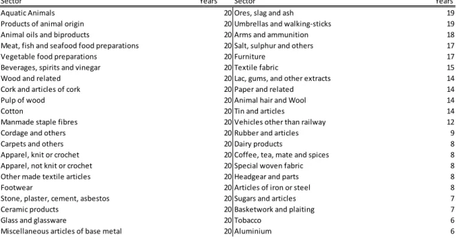
Table 3 Competitive Sectors
Table 4 Unit Root Tests Table 5 Variable Descriptive Statistics
Sector Years Sector Years
Aquatic Animals 20 Ores, slag and ash 19
Products of animal origin 20 Umbrellas and walking-sticks 19
Animal oils and biproducts 20 Arms and ammunition 18
Meat, fish and seafood food preparations 20 Salt, sulphur and others 17
Vegetable food preparations 20 Furniture 17
Beverages, spirits and vinegar 20 Textile fabric 15
Wood and related 20 Lac, gums, and other extracts 14
Cork and articles of cork 20 Paper and related 14
Pulp of wood 20 Animal hair and Wool 14
Cotton 20 Tin and articles 14
Manmade staple fibres 20 Vehicles other than railway 12
Cordage and others 20 Rubber and articles 9
Carpets and others 20 Dairy products 8
Apparel, knit or crochet 20 Coffee, tea, mate and spices 8
Apparel, not knit or crochet 20 Special woven fabric 8
Other made textile articles 20 Headgear and parts 8
Footwear 20 Articles of iron or steel 8
Stone, plaster, cement, asbestos 20 Sugars and articles 7
Ceramic products 20 Basketwork and plaiting 7
Glass and glassware 20 Tobacco 6
Miscellaneous articles of base metal 20 Aluminium 6
Number of Years between 1988 and 2007 Portugal had a revealed competitive advantage
Variable p-value Variable p-value
d_r_y 0.0343 exsample -d_oil_wti - d_psi -d_def - d_ot 0.0063 d_tdir 0.0007 e1 -d_tindr - e2 -d_lsnf 0.1836 e3 -d_lhouse 0.0287 d_kh 0.0019 d_loan 0.4531 d_kw -d_tot 0.0002 d_kl -d_fdi2 - dtheta 0.0001 d_rce 0.0022 d_ip 0.0107 d_ulc 0.0001 d_cpi 0.0001 d_cepop 0.0057 d_cpi_c 0.0008 d_cewpop 0.0027 d_cpi_d 0.0009 excomp - t 0.0021 - Indicates 0
Phillips Perron test Variable Observations Mean Std. Dev. Min Max
d_r_y 35 2.276 2.849 -3.315 7.816 d_kw 36 0.026 0.017 -0.014 0.071 d_kl 35 0.012 0.064 -0.150 0.178 d_rce 37 1.240 3.153 -7.125 8.920 d_cepop 37 5.415 8.107 -9.564 23.831 d_cewpop 37 4.966 8.209 -11.417 26.024 excomp 37 5.348 4.808 -12.319 14.434 exsample 37 5.919 4.329 -11.212 13.564 d_loan 34 12.936 9.623 -5.538 27.353 d_cpi_c 36 0.041 0.058 -0.090 0.225 d_cpi_d 36 0.040 0.059 -0.090 0.225
Page 22 of 25
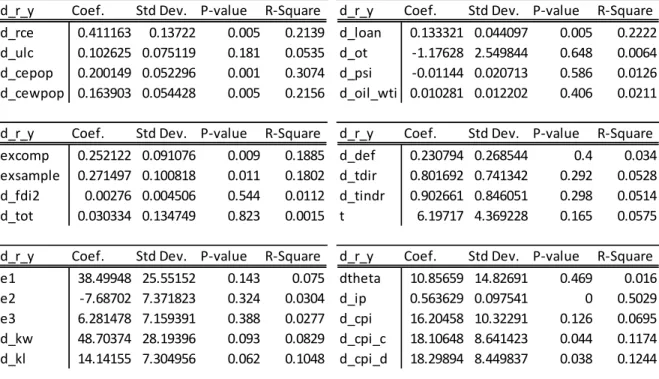
Table 6 Initial Regressions
Table 7 Second Regressions
d_r_y Coef. Std Dev. P-value R-Square d_r_y Coef. Std Dev. P-value R-Square d_rce 0.411163 0.13722 0.005 0.2139 d_loan 0.133321 0.044097 0.005 0.2222 d_ulc 0.102625 0.075119 0.181 0.0535 d_ot -1.17628 2.549844 0.648 0.0064 d_cepop 0.200149 0.052296 0.001 0.3074 d_psi -0.01144 0.020713 0.586 0.0126 d_cewpop 0.163903 0.054428 0.005 0.2156 d_oil_wti 0.010281 0.012202 0.406 0.0211
d_r_y Coef. Std Dev. P-value R-Square d_r_y Coef. Std Dev. P-value R-Square excomp 0.252122 0.091076 0.009 0.1885 d_def 0.230794 0.268544 0.4 0.034 exsample 0.271497 0.100818 0.011 0.1802 d_tdir 0.801692 0.741342 0.292 0.0528 d_fdi2 0.00276 0.004506 0.544 0.0112 d_tindr 0.902661 0.846051 0.298 0.0514
d_tot 0.030334 0.134749 0.823 0.0015 t 6.19717 4.369228 0.165 0.0575
d_r_y Coef. Std Dev. P-value R-Square d_r_y Coef. Std Dev. P-value R-Square
e1 38.49948 25.55152 0.143 0.075 dtheta 10.85659 14.82691 0.469 0.016 e2 -7.68702 7.371823 0.324 0.0304 d_ip 0.563629 0.097541 0 0.5029 e3 6.281478 7.159391 0.388 0.0277 d_cpi 16.20458 10.32291 0.126 0.0695 d_kw 48.70374 28.19396 0.093 0.0829 d_cpi_c 18.10648 8.641423 0.044 0.1174 d_kl 14.14155 7.304956 0.062 0.1048 d_cpi_d 18.29894 8.449837 0.038 0.1244 Regressions Model 1 2 3 4 5 6 7 L.d_r_y 0.011 0.008 0.051 0.015 0.001 0.011 0.003 d_kw 0.181 0.071 0.352 d_kl 0.009 0.043 0.056 0.107 d_rce 0.000 0.000 d_cepop 0.000 0.000 0.000 0.000 d_cewpop 0.000 excomp 0.000 0.001 0.000 0.000 0.000 exsample 0.000 0.000 d_loan 0.096 0.138 0.317 d_cpi_c 0.580 0.172 0.000 0.000 0.001 0.000 d_cpi_d 0.000 Adj R-squared 0.693 0.734 0.800 0.821 0.726 0.803 0.783 bgodfrey 0.18 0.89 0.86 0.14 0.05 0.22 0.85 hettest 0.37 0.83 0.05 0.25 0.58 0.17 0.19 VIF 1.70 1.51 2.64 2.50 2.29 2.51 2.67 Ramsey RESET 0.78 0.59 0.56 0.92 0.52 0.97 1.00 dwatson 1.59 0.19 2.01 2.36 2.51 2.35 2.04 Signficance
Page 23 of 25
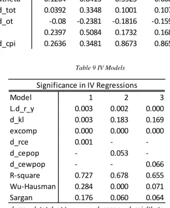
Table 8 Correlations Table
Table 9 IV Models
Corr d_r_y d_rce d_cepop d_cewpop
dtheta 0.1264 0.8413 0.5925 0.6088 d_tot 0.0392 0.3348 0.1001 0.1075 d_ot -0.08 -0.2381 -0.1816 -0.1595 t 0.2397 0.5084 0.1732 0.1684 d_cpi 0.2636 0.3481 0.8673 0.8653 Model 1 2 3 L.d_r_y 0.003 0.002 0.000 d_kl 0.003 0.183 0.169 excomp 0.000 0.000 0.000 d_rce 0.001 - -d_cepop - 0.053 -d_cewpop - - 0.066 R-square 0.727 0.678 0.655 Wu-Hausman 0.284 0.000 0.071 Sargan 0.176 0.060 0.064
d_rce = d_tot d_ot t d_cepop = d_cpi dtheta d_cewpop = d_cpi dtheta
Page 24 of 25
Table 10 Final Model
Table 11 Model with growth in Tradable ratio
_cons -.5665935 .4353662 -1.30 0.204 -1.458401 .3252136 excomp .1945289 .0509563 3.82 0.001 .0901497 .2989082 d_rce .3860143 .0900762 4.29 0.000 .2015016 .570527 d_kl 12.35776 4.591537 2.69 0.012 2.952419 21.7631 L1. .4354317 .1045375 4.17 0.000 .2212963 .6495671 d_r_y d_r_y Coef. Std. Err. t P>|t| [95% Conf. Interval] Total 232.067949 32 7.25212341 Root MSE = 1.4295 Adj R-squared = 0.7182 Residual 57.2148353 28 2.04338698 R-squared = 0.7535 Model 174.853114 4 43.7132784 Prob > F = 0.0000 F( 4, 28) = 21.39 Source SS df MS Number of obs = 33
_cons -.6294011 .5807395 -1.08 0.304 -1.923369 .6645672 L1. .4268289 .1692766 2.52 0.030 .0496572 .8040006 d_r_y d_trade -51.7089 55.52871 -0.93 0.374 -175.4346 72.01677 d_rce .6597826 .2379323 2.77 0.020 .1296364 1.189929 d_kl 14.26114 8.076782 1.77 0.108 -3.735047 32.25734 excomp .1882943 .0587143 3.21 0.009 .0574706 .319118 d_r_y Coef. Std. Err. t P>|t| [95% Conf. Interval] Total 75.2998608 15 5.01999072 Root MSE = 1.1556 Adj R-squared = 0.7340 Residual 13.3544412 10 1.33544412 R-squared = 0.8226 Model 61.9454196 5 12.3890839 Prob > F = 0.0016 F( 5, 10) = 9.28 Source SS df MS Number of obs = 16
Page 25 of 25
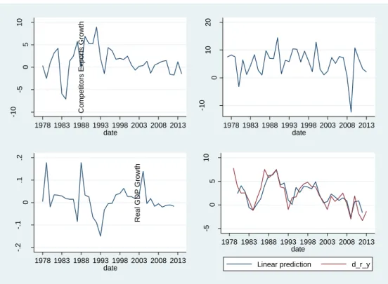
Figure 1 Growth of Model and Explanatory Variables
Figure 2 Model and Explanatory Variables
-1 0 -5 0 5 10 R C E Gr o w th 1978 1983 1988 1993 1998 2003 2008 2013 date -1 0 0 10 20 C o m p e ti to rs E x p o rt s Gr o w th 1978 1983 1988 1993 1998 2003 2008 2013 date -. 2 -. 1 0 .1 .2 C a p it a l p e r e ff e c ti v e l a b o r 1978 1983 1988 1993 1998 2003 2008 2013 date -5 0 5 10 R e a l GD P Gr o w th 1978 1983 1988 1993 1998 2003 2008 2013 date
Linear prediction d_r_y
60 70 80 90 100 R e a l C o m p e n s a ti o n o f E m p lo y e e s 1978 1983 1988 1993 1998 2003 2008 2013 date 0 2 4 6 8 C o m p e ti to rs E x p o rt s 1978 1983 1988 1993 1998 2003 2008 2013 date Competitors World .0 3 .0 3 5 .0 4 .0 4 5 .0 5 C a p it a l p e r e d u c a te d l a b o r 1978 1983 1988 1993 1998 2003 2008 2013 date 100 150 200 250 GD P v s M o d e l 1978 1983 1988 1993 1998 2003 2008 2013 date RealGDP Prediction