A dynamic programming approach for evaluating a portfolio of R&D projects with a budget

SOP TRANSACTIONS ON APPLIED MATHEMATICS

A Dynamic Programming Approach for

Evaluating A Portfolio of R&D Projects with

A Budget

Anabela Costa

_{* , Jos´e Pinto Paix ˜ao}

1_{Instituto Universit´ario de Lisboa (ISCTE IUL), Portugal Centro de Investigac ˜ao Operacional, Portugal.} 2_{Faculdade de Ci `encias da Universidade de Lisboa, Portugal Centro de Investigac ˜ao Operacional, Portugal.}

*Corresponding author: anabela.costa@iscte.pt

Abstract:

The Real Options approach has proved to be a suitable methodology for capturing the flexibility in the investment decision process. This is very useful for the financial evaluation of R&D projects where there are several possible decisions concerning to the investment – delaying, improving or abandoning. Since the risk of an R&D project is usually due to singular characteristics of the project and is uncorrelated with the financial markets, the contingent claims analysis may be not adequate to value R&D projects. Based on a dynamic programming evaluation model, presented in Huchzermeier and Loch [1], we propose an approach to valuing a portfolio of R&D projects with a budget. Specifically, considering a budget constraint, we make an extension of the model mentioned above for assessing the projects in the portfolio simultaneously. To test the proposed evaluation procedure, we generated several R&D portfolios with different dimensions and characteristics. According to our computational experience, the main conclusions are presented.

Keywords:

Stochastic Dynamic Programming; Project Valuation; R&D Project; Real Options

1. INTRODUCTION

From the range of investment projects stand out the research and development projects (R&D projects), which are extremely important in some economy sectors as the pharmaceutical and high tech industries, in order to create new products or services. These projects should be viewed as a collection of sequential decisions, which involve a R&D phase, multi-stage, and a commercialization phase, with different risks and uncertainties, which will decreasing as the project develops [2,3].

The structure of the flexible decision of real options is valid in R&D projects. Specifically, after an initial investment it is possible collect more information on the evolution of the project and market conditions and, based on this information, modify the action plan [1,3–7].

In most cases, the R&D projects are associated with the development of innovative products for which there are no market benchmarks. Since the underlying asset of the option on the R&D project is not

traded, the respective market value cannot be determined [8]. For this reason, the contingent claims analysis, which is based on the principle of replication, should not be applied to evaluate R&D projects [3]. An alternative technique for evaluating real options is dynamic programming, which is not based on the principle of replication of the risks of the underlying asset [4,9]. However, with this technique, the discount rate that reflects the risk attitude of the decision maker has to be specified exogenously [1]. On the other hand, the risk associated with a R&D project is normally attributed to the intrinsic characteristics of the project, that is, the risk is unsystematic or diversifiable. In this way, many researchers argue that a reasonable hypothesis for a large company is a neutral attitude to the risk of the project with the discounted process at the risk-free interest rate [1,3,4,9,10].

In this perspective, in Huchzermeier and Loch [1] is developed a dynamic programming model to evaluate a R&D project. In order to react to the arrival of new information on the evolution of the project, there are two options at each stage of R&D phase: abandon the project or continue the project with an improvement action. Based on a set of levels of performance expected for the project, the backward recursion procedure determines, in each stage of the R&D phase, the value of the project for each of these performance levels.

In this paper, we present a procedure to evaluate a portfolio of R&D projects considering a limited budget for improvement actions. We generalize the evaluation of Huchzermeier and Loch [1]. Specifically, to evaluate simultaneously several R&D projects, we assume that the performance level of a project at every stage of R&D phase is independent of the level reached by other projects. This assumption implies that, at each stage of R&D phase, the evaluation of a project in a given performance level requires the calculation of its combined value (that is, the value of the project, when we considered simultaneously all projects of the portfolio) in each of the feasible performance levels to each one of the other projects. This process can be time consuming when there are many projects and the number of stages of the phase R&D is high.

Next section of the paper reports the main features of a R&D project. In the following section, we review the dynamic programming model presented in Huchzermeier and Loch [1]. The Sect. 4 is devoted to the presentation of the evaluation procedure which enable evaluate a portfolio of R&D projects subject to a budget constraint for improvement actions. While in Sect. 5 is given an example of application of the proposed approach. Computational experience is reported in Sect. 6 and some final comments are made in the last section of the paper.

2. CHARACTERIZATION OF A R&D PROJECT

The financial evaluation of R&D projects assumes great importance in industrial sectors that are dedicated to research and development of innovative products or services. Among the various industries, stand out the pharmaceutical and high technology industries. Several studies have demonstrated that a R&D project can be evaluated through a real options analysis. For example, Pennings and Sereno [11] presented a compound option approach for evaluating pharmaceutical R&D investments projects in the presence of technical and economic uncertainties. Lee [12] established a real option analysis approach to value renewable energy investments, concretely, a wind energy technology. Kellogg and Charnes [13] proposed a real option analysis procedure, based on binomial models, to value companies and projects in the biotech industry. Herath and Park [14] presented a discrete binomial model to value the project of a new product in the consumer goods industry.

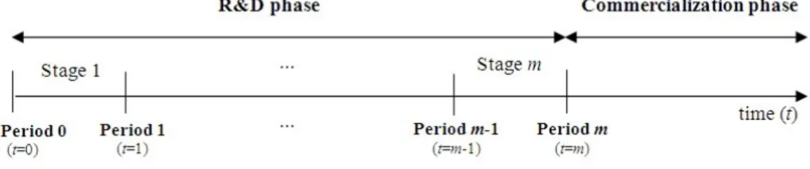
Figure 1. Interpretationof a R&D project [2]

According to [2], a R&D project should be interpreted as a collection of sequential decisions, which involve the phase of research and development and a commercialization phase (seeFigure 1). At each phase, it is assumed that there are different risks and uncertainties, which will decreasing as the project evolves. Still, according to these authors, the purpose of an R&D is to maximize future revenues or minimize future costs.

When a company accepts an R&D project, through the payment of an initial premium, the first stage of the R&D phase is initiated and the company acquires the right (that is, the option) to decide if the project proceeds to second stage; if the second stage of R&D phase is initiated, upon payment of a second premium, the company gains the opportunity to continue to the third step, and so on. Therefore, an investment opportunity in a R&D project can be viewed as a compound option (that is, an option that to be exercised activates new options) [15,16].

The flexibility of decision associated with each stage of the R&D project is not limited to the option of abandoning the project [17]. Also it is possible choose to defer the decision on the project until more information is available on the investment [18], or expand or contract the project [19,20], or even change the operating mode of the project depending on the price factor [21]. In Huchzermeier and Loch [1] has been introduced a new type of flexibility, which translates into the option of performing, at every stage of R&D phase, an improvement action.

The R&D projects are characterized by a long-term horizon and a high degree of uncertainty, of a technical nature (due to the characteristics of the projects) and market. Therefore the value of decision flexibility in a R&D project (that is, the value of an option on a R&D project) can be substantial [3,5]. The two types of uncertainty influence differently the value of flexibility underlying a R&D project. Indeed, the technique uncertainty reduces the value of flexibility, since it is very likely that the operating costs will increase. While the market uncertainty leads to an increase in the value of flexibility, since there is possibility of high returns, which can be upgraded with the possibility of other uses for the created knowledge [1].

3. DYNAMIC PROGRAMMING MODEL OF HUCHZERMEIER AND LOCH

(2001)

Before presenting the evaluation model developed in Huchzermeier and Loch [1], we define the R&D project of the model and we identify the uncertainty factors that affect its value, and therefore its option value.

Figure 2. Scheme of the R&D project relating to the evaluation model

3.1 R&D project of the evaluation model

The R&D project considered in the evaluation model consists of the phases R&D and of commercial-ization. The R&D phase is composed of m stages with the same duration (seeFigure 2).

The acceptance of a R&D project involves an initial capital outlay, I, to acquire the necessary infrastruc-tures to start the project. At the beginning of each stage of the R&D phase (review period of the project), according to most recent information, there is an opportunity to abandon, continue or improve the project. In period t=0,. . . ,m 1, the continuity decision requires the payment of a cost ct while the improvement

decision requires the payment of the cost ctand a cost of improvement dt. If the m stages are performed

(that is, if the project was not abandoned at some stage) then is necessary to decide the passage or not, to commercialization phase.

For example, the scheme associated with creating a new drug is the following: the starting point is a research stage that covers the biological validation of the drug target and the subsequent chemical optimization of the potential drug candidate. Moving forward to early development, pre-clinical phase mainly comprises animal testing. The main goals of pre-clinical studies are to understand adverse effects of the drug during clinical trials. If these tests are successful, the new drug application must be submitted to the public health agency (FDA-Food and Drug Administration or EMEA-European Medicines Agency) for the approval to starting testing in humans. Following a positive decision, the compound is administered to healthy volunteers in clinical phase I to gather information about safety dosage. In clinical phase II, application to a small number of patients is done to obtain proof of the concept. The next step of late development is characterized by clinical phase III studies that include a larger number of patients to ensure statistical significance. After successful completion, a new drug application is submitted to the agency for marketing approval. If the drug is approved it becomes available for patients [11,22].

The value of the R&D project depends on several factors of uncertainty, which will be listed in the next section.

3.2 Uncertainty factors considered in the evaluation model

A R&D project is characterized by the time associated to R&D phase, cost over time and by the performance of the resulting product. In turn, the market is characterized by the return from the project (caused by the size and attractiveness of the market) and by the performance requirements (which indicate how the return increases with the performance of the product). The interaction of project characteristics with the market characteristics contributes decisively to the value of the R&D project. Therefore, the

value of a R&D project is function of the factors: time, cost, performance, market return and market requirements.

In the evaluation model developed in Huchzermeier and Loch [1] is assumed that the R&D project can be defined in terms of the expected performance along a corridor or cone of performance states during the time of development, a fixed range of market returns (for example, market returns that belong to the range [u, U], u, U2¬) and a range of market requirements.

Although the evaluation model only considers three factors of uncertainty, in Huchzermeier and Loch [1] is studied the influence of each of the five risk factors in the value of the R&D project.

The following sections provide the modeling of each of the uncertainty factors that define the value of the R&D project.

3.2.1 Modeling of the performance associated to the product resulting

Given the uncertainty, the product performance, designated by i, it changes between periods of project review. In each review period, the R&D teams perform corrections to the project plan, where the expected performance is estimated from tests, simulations or prototypes [23]. Thus, for each period t=0,...,m, we define the system of product performance states by (t, i), where i is a level of performance for the product under development.

Huchzermeier and Loch [1] admit that the performance in each period t=0,...,m 1, follows a Binomial distribution, regardless of the history associated with the development of the project. Specifically, the product performance of period t=0,...,m 1 for the period t+1

1. may improve in 1/2, with probability p, or may decrease by 1/2, with probability 1 p, with a continuity action; or

2. may improve in 3/2, with probability p, or may improve by 1/2, with probability 1 p, with an improvement action.

These two types of action lead to a recombined tree that defines the set of feasible performance levels for the product under development. Specifically, Ptis the set of feasible performance levels in time period

t=0,...,m (it is assumed that the level of performance at t=0, i0, i02¬, is known, therefore P0={i0}). To a

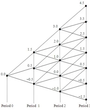
better understanding of the generation of the performance levels, we present inFigure 3the recombined tree that defines the feasible levels of performance, in each period t, for the product associated with a project whose R&D phase consists of m=3 stages.

In this paper, we consider this scheme of evolution for the performance of the product, however the authors generalize the binomial distribution, allowing that the improvement performance and the regression performance, respectively, are expanded by the next N (which represents a natural number) performance states.

Figure 3. Recombined tree that defines the levels of performance for a project with m=3 stages in the R&D phase, assuming the level of performance i0=0 at period t = 0. Each node of the tree is a feasible level of

performance i for the product associated with the project. For example, at t=0, the decision continue the project will lead to the levels 0.0+0.5 or 0.0-0.5 at t=1; otherwise, the decision improve the project will lead to the levels 0.0+0.5 or 0.0+1.5 at t=1. According with the recombined tree, P1={-0.5,0.5,1.5},

P2={-1.0,0.0,1.0,2.0,3.0} and P3={-1.5,-0.5,0.5,1.5,2.5,3.5,4.5}.

3.2.2 Modeling of the market return and of the market requirements

After the R&D phase (that is, in period m), the product is launched on the market with a performance level i, which will produce an expected market return

p(i) = u + F(i) ⇥(U u) (1) Where [u, U], u, U2¬, is the range of market returns and F(i) denotes the probability distribution function of the random variable D, which represents the level of performance required by the market. Huchzermeier and Loch [1] assumes that D follows the Normal distribution of parameters (µ, s).

At this point, it is possible present the model that allows determine the value of the R&D project.

3.3 Evaluation Model

The evaluation of a R&D project corresponds to a sequential decision problem, which can be formulated as a stochastic dynamic program.

The value of the R&D project depends on the level of performance i, and thus at each time period t we need to calculate the value V(t, i), i2Pt, t=0,...,m. The valuation procedure requires starting at time period

t=m and working backwards through time in the standard dynamic programming fashion. At period

Table 1. Dynamic Programming Procedure of Huchzermeier and Loch [1] begin

V(m,i) p(i), i2Pm;

for t=m 1 to 0 do for i2Ptdo V (t,i) Max 8 > < > : 0, (decision : abandon)

ct+p⇥V(t+1,i+0.5)+(1 p)⇥V(t+1,i 0.5)1+r , (decision : continue)

ct dt+p⇥V(t+1,i+1.5)+(1 p)⇥V(t+1,i+0.5)_1+r (decision : improve) end;

end; end.

t=m the value V(m, i), i2Pm, corresponds to the expected market return if the product is launched on the

market with the performance level i,p(i), defined by (1).

At another period t=0, 1,..., m 1, the value V(t, i), will depend on the investment decision at the level of performance i2Pt, and the corresponding value of the R&D project at period t+1. Therefore, we must

select the investment decision (abandon, continue or improve) that maximizes the value of the project. The R&D project value at period t, given each of the three possible investment decisions is

V (t,i) = Max 8 > < > : 0, (decision : abandon) ct+p⇥V(t+1,i+0.5)+(1 p)⇥V(t+1,i 0.5)_1+r , (decision : continue)

ct dt+p⇥V(t+1,i+1.5)+(1 p)⇥V(t+1,i+0.5)_1+r , (decision : improve)

(2)

For example, the decision of continue involves the continuity cost ctand the discounted value of the

expected value at the next period. The expected value is based on the two branches emanating from node i at period t and the associated probabilities p and (1 p). Note that it is used the risk-free rate r to discount.

Once the dynamic programming procedure is completed, V(0,i), i2P0, represents the value of the R&D

project at period t=0 before being subtracted from the initial investment, I. Therefore, V(0,i) I, i2P0,

represents the optimal value of the R&D project at the present moment. In general, if the expected value V(0,i) I, i2P0, is greater than or equal to zero the R&D project should be developed.

Table 1presents a resume of the dynamic programming procedure of Huchzermeier and Loch [1].

4. GENERALIZATION OF THE HUCHZERMEIER AND LOCH MODEL

To evaluate an investment portfolio composed of n R&D projects, which is subject to a budget constraint for improvement actions, we propose an approach that generalizes the Huchzermeier and Loch model [1]. The R&D projects considered in the portfolio have the characteristics mentioned in Sect. 3.1 and the respective R&D phases are composed of m stages. The parameters of each project j=1,. . . ,n are presented inTable 2. Given the complexity of this evaluation problem, it will not be possible to obtain the optimal value of each project but only an estimate for the value of each project.

Assuming the existence of a limited budget Btat each period t=0,...,m 1 for improvement decisions,

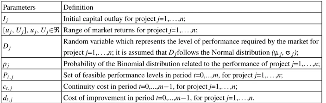
Table 2. Parameters of the Projects Parameters Definition

Ij Initial capital outlay for project j=1,. . . ,n;

[uj, Uj], uj, Uj2¬ Range of market returns for project j=1,. . . ,n;

Dj Random variable which represents the level of performance required by the market for

project j=1,. . . ,n; it is assumed that Djfollows the Normal distribution (µj,sj);

pj Probability of the Binomial distribution related to the performance of project j=1,. . . ,n;

Pt, j Set of feasible performance levels in period t=0,...,m, for project j=1,. . . ,n;

ct, j Continuity cost in period t=0,...,m 1, for project j=1,. . . ,n;

dt, j Cost of improvement in period t=0,...,m 1, for project j=1,. . . ,n.

respect the available budget. Therefore, at each time period t=0,...,m we must determine VPj(t,i), that is,

the value in parallel of R&D project j=1,. . . ,n, for each performance level i2Pt, j, considering that at each

time period the performance level associated with a project is independent of the level achieved for the remaining projects.

At period t=m the value VPj(m, i), i2Pm, j, j=1,. . . ,n, corresponds to the expected market return if the

product, relating to project j, is launched on the market with the performance level i,

pji = uj+Fj(i) ⇥ (Uj uj) (3)

where Fj(i) denotes the probability distribution function of the random variable Dj.

For another period t=0,. . . ,m 1, the value VPj(t, i), i2Pt, j, j=1,. . . ,n, will depend on the individual

investment decision for project j at the performance level i. Therefore, we must select the decision (abandon, continue or improve) that maximizes the individual value of project j at the level of performance i, Vj(t, i), that is, the value of project j when evaluated individually at the level of performance i. Assuming

that the budget Btallows at least an improvement decision, the individual value is determined according

with (4): Vj(t,i) = Max 8 > < > : 0, (abandon)

ct, j+pj⇥V Pj(t+1,i+0.5)+(1 p_1+r j)⇥V Pj(t+1,i 0.5), (continue)

ct, j dt, j+pj⇥V Pj(t+1,i+1.5)+(1 p_1+r j)⇥V Pj(t+1,i+0.5), (improve)

(4)

For example, the decision of improve involves the continuity cost ct, j, the improvement cost dt, j, and

the discounted value of the expected parallel value at the next period. The expected value is based on the two branches emanating from node i at period t and the associated probabilities pjand (1 pj). As in the

model of Huchzermeir and Loch [1], it is used the risk-free rate r to discount.

Since only improvement decisions are subject to the budget Bt, the value in parallel of project j at the

performance level i, VPj(t, i), is equal to the respective individual value Vj(t, i), when the individual

decision for project j at the state (t, i) is abandon or continue.

Case the individual decision for the project j in the state (t, i) is improve, we have to check if it is possible keep this decision in the evaluation in parallel of the n projects. Concretely, we must determine the combined value Vj(t, i, c) of project j in state (t, i) for each combination of performance levels c of the

remaining projects. Where c is a vector with n 1 components, wherein the component k has a feasible level of performance ik2Pt,kfor the project k=1,...,n, k6=j. Such evaluation requires the definition of a

criterion to select the projects that should be improved when the budget Bt, t=0,. . . ,m 1, is not sufficient

for the volume of improvement individual decisions. We establish that Bt, t=0,. . . ,m 1, must be allocated

to projects that have the highest individual value. According to this criterion, for each combination of levels of performance c, the budget begins to be allocated to projects that have an individual decision of improve and a higher individual value than the project j. After this budget allocation, if the available budget is sufficient to improve the project j then the combined value of project j in state (t, i) for the combination of performance levels c, Vj(t, i, c), is equal to the individual value Vj(t, i); otherwise, the

combined value of project j in state (t, i) for the combination of performance levels c is

Vj(t,i,c) = Max

(

0, (abandon)

ct, j+ [pj⇥V Pj(t + 1,i + 0.5) + (1 pj)⇥V Pj(t + 1,i 0.5)] (1 + r) (continue)

(5) Once the combined value of project j in state (t, i) is determined for all the combinations of performance levels c, the value in parallel of project j at the performance level i, VPj(t, i), corresponds to the combined

value of project j most common.

When the dynamic programming procedure is completed, VPj(0,i), i2P0, j, represents the parallel

value of the R&D project j=1,. . . ,n at period t=0 before being subtracted from the initial investment, Ij.

Therefore, VPj(0,i) Ij, i2P0, j, represents an estimate for the value of the R&D project j=1,. . . ,n at the

present moment, when evaluating simultaneously n projects subject to a budget Bt, for improvement

actions, in each period t=0,. . . ,m 1. Generally, the holder of the portfolio should develop the projects whose estimated values, VPj(0,i) Ij, i2P0, j, j=1,. . . ,n, are greater than or equal to zero.

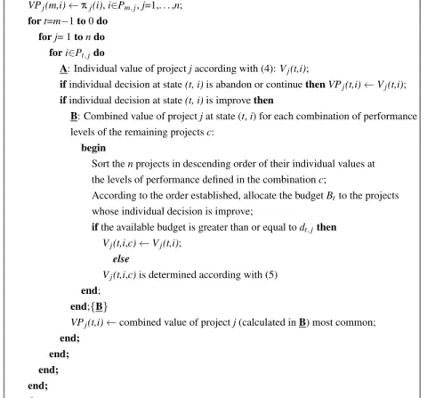
Table 3presents a resume of the dynamic programming procedure developed.

Possible practical applications of this approach are, for example, in a pharmaceutical company, the development of multiple drugs that could potentially treat a specific disease; in an auto manufacturer, the development of several prototypes for a new car design; or, in a communications company, the development of several techniques to create a new microwave relay system.

5. Example

The following example illustrates the dynamic programming approach proposed in this paper to evaluate an investment portfolio composed of n R&D projects, which is subject to a budget constraint for improvement actions. Let us consider a portfolio with three R&D projects described inTable 4and a risk-free interest rate r=8%.

The R&D phases of the three projects are composed by m=3 stages. Finally, the costs of continuity and of improvement as well as the budget for improvement actions in each period t=0,1,2 are presented in

Table 5.

Assuming that in period t=0, the performance level of each of the three projects is 0, we start by evaluating each project individually.

The evaluation of each project is presented in Figure 4, which enables to state that the val-ues of the projects 1, 2 and 3, in the period t=0 are, respectively, V1(0,0) I1=206.1 87=119.1,

Table 3. Dynamic Programming Procedure Developed begin

VPj(m,i) pj(i), i2Pm, j, j=1,. . . ,n;

for t=m 1 to 0 do for j= 1 to n do

for i2Pt, jdo

A: Individual value of project j according with (4): Vj(t,i);

if individual decision at state (t, i) is abandon or continue then VPj(t,i) Vj(t,i);

if individual decision at state (t, i) is improve then

B: Combined value of project j at state (t, i) for each combination of performance levels of the remaining projects c:

begin

Sort the n projects in descending order of their individual values at the levels of performance defined in the combination c;

According to the order established, allocate the budget Btto the projects

whose individual decision is improve;

if the available budget is greater than or equal to dt, jthen

Vj(t,i,c) Vj(t,i);

else

Vj(t,i,c) is determined according with (5)

end; end;{B}

VPj(t,i) combined value of project j (calculated in B) most common;

end; end; end; end; end.

Table 4. Parameters for the R&D projects

Project j Initial capital outlay Ij Parameters of Normal distribution (µj,sj) Range of market returns [uj, Uj] Probability pj

1 87 (0.0,2.0) [5, 490] 0.5

2 98 (0.0,2.0) [8, 478] 0.5

3 77 (0.0,2.8) [0, 490] 0.5

projects, the optimal decision in period t=0 (that is, at the beginning of stage 1) is improve. According to this evaluation, each project adds value to the company and, if desired, the projects can be developed.

Now we will evaluate the three projects simultaneously by applying the dynamic programming proce-dure developed. To exemplify the evaluation proceproce-dure, we calculate the estimate for the parallel value of the project 1 at the period t=2 for the level of performance i= 1 (that is, V1(2, 1)). According with (4),

the individual value of the project 1 at the period t=2 for the level of performance i= 1 is

Table 5. Costs of continuity, improvement and budget for improvement actions in period t=0,1,2 Period t ct,1 dt,1 ct,2 dt,2 ct,3 dt,3 Bt

0 10.0 17.0 14.0 17.0 9.0 22.0 35 1 26.0 32.0 23.0 28.0 20.0 45.0 58 2 39.0 64.0 34.0 53.0 36.0 70.0 80

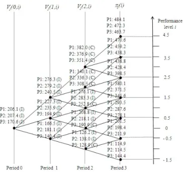
Figure 4. Recombined tree which translates the possible levels of performance for the n=3 projects in each period t=0,1,2,3. In each state (t, i) of the tree, we present the value of project j, when it is evaluated individually, at each performance level i, Vj(t,i), t=0,1,2, j=1,2,3, i 2 Pt, j, and the respective decision (A: abandon; C:

continue; I: improve). V1(2, 1) 126.2 = Max 8 > < > : 0 39 + (0.5 ⇥ 114.9 + 0.5 ⇥ 201.5) 1.08 39 64 + (0.5 ⇥ 201.5 + 0.5 ⇥ 293.5) 1.08 (6)

and the associated decision is improve. To determine de value of the project 1 at the period t=2 for the level of performance i= 1, considering the simultaneous evaluation, we must compute the combined value of project 1 at the state (t, i)=(2, 1) for each of the 25 combinations of performance levels c of the remaining two projects. For example, in the combination of levels of performance c=( 1, 1), where projects 2 and 3 achieved the performance level 1, the project 2 has the higher individual value and is relating to an improvement decision (seeFigure 4), therefore the budget B2=80 should be assigned to

project 2. Since the remaining budget, B2 d2,2=27, is not sufficient to improve project 1, the value of

project 1 at the state (t, i)=(2, 1) for the combination c=( 1, 1) is determined according to (5):

V1(2, 1,c) 107.5 = Max

( 0

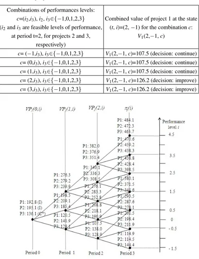
39 + (0.5 ⇥ 114.9 + 0.5 ⇥ 201.5) 1.08 (7) and the associated decision is continue. For the others combinations of performance levels of projects 2 and 3, the process is analogous. InTable 6, we resumed the 25 combined values for project 1 at the state (t, i)=(2, 1). As the combined value most common is 107.5, the estimate for the parallel value of project 1 at the period t=2 for the level of performance i= 1 is VP1(2, 1)=107.5.

After applying this procedure to all the projects and levels of performance, we obtain the evaluation results shown inFigure 5.

Table 6. Combined values for project 1at the state (t, i)=(2, 1) Combinations of performances levels:

c=(i2,i3), i2, i32{ 1,0,1,2,3}

(i2and i3are feasible levels of performance,

at period t=2, for projects 2 and 3, respectively)

Combined value of project 1 at the state (t, i)=(2, 1) for the combination c:

V1(2, 1, c)

c= ( 1,i3), i32{ 1,0,1,2,3} V1(2, 1, c)=107.5 (decision: continue)

c= (0,i3), i32{ 1,0,1,2,3} V1(2, 1, c)=107.5 (decision: continue)

c= (1,i3), i32{ 1,0,1,2,3} V1(2, 1, c)=107.5 (decision: continue)

c= (2,i3), i32{ 1,0,1,2,3} V1(2, 1, c)=126.2 (decision: improve)

c= (3,i3), i32{ 1,0,1,2,3} V1(2, 1, c)=126.2 (decision: improve)

Figure 5. Application of the dynamic programming procedure developed. In each state (i, t) of the tree, we present an estimate for the parallel value of project j, when it is evaluated simultaneously with the remaining projects, at each performance level i, V Pj(t,i), t=0,1,2, j=1,2,3, i 2 Pt, j. For the state (0,0) we present the

decision proposed for each project (A: abandon; C: continue; I: improve; C* or A*: continue or abandon, when in the simultaneous evaluation is not possible keep the improvement decision determined in the individual evaluation).

According to the evaluation procedure developed, the estimates for the parallel values of the projects 1, 2 and 3, in period t=0 are, respectively, VP1(0,0) I1=105.8, VP2(0,0) I2=97.1 and VP3(0,0) I3=59.1.

With respect to the decision policy in period t=0, we can say that, for projects 1 and 2 the decision proposed is improve, while for project 3 the decision proposed is continue. In comparison with the individual values obtained for the period t=0, we can say that the respective estimated values of the projects, when subjected to a simultaneous evaluation, suffer reductions, being the highest recorded in the third project. Moreover, the decision in period t=0 associated with the project 3 is reviewed: the improvement decision of the individual evaluation is replaced by a continuity decision. These conclusions were predictable, since the budget Bt, t=0,1,2, is not enough to keep all the improvement decisions established on individual

evaluation. However, each project continues to add value to the company, which means that the holder of the portfolio can start in parallel the development of the three projects (specifically, projects 1 and 2 start with an improve decision, while the decision for project 3 is continue).

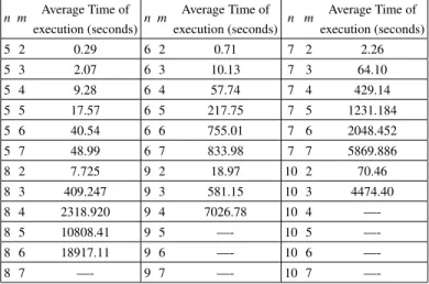
Table 7. Average execution time associated to the evaluation approach developed. For each pair (n, m), n=5,...,10 and m=2,...,7, are evaluated seven instances.

n m Average Time of execution (seconds) n m Average Time of execution (seconds) n m Average Time of execution (seconds) 5 2 0.29 6 2 0.71 7 2 2.26 5 3 2.07 6 3 10.13 7 3 64.10 5 4 9.28 6 4 57.74 7 4 429.14 5 5 17.57 6 5 217.75 7 5 1231.184 5 6 40.54 6 6 755.01 7 6 2048.452 5 7 48.99 6 7 833.98 7 7 5869.886 8 2 7.725 9 2 18.97 10 2 70.46 8 3 409.247 9 3 581.15 10 3 4474.40 8 4 2318.920 9 4 7026.78 10 4 —-8 5 10808.41 9 5 —- 10 5 —-8 6 18917.11 9 6 —- 10 6 —-8 7 —- 9 7 —- 10 7

—-6. COMPUTATIONAL EXPERIENCE

We conducted computational experiments for a total of 252 test instances, with the number of projects varying from 5 to 10 and a number of stages in the R&D phase ranging between 2 and 7. Specifically for each test problem of dimension (n, m), n=5,. . . ,10 and m=2,. . . ,7, we generate seven instances with different percentages of improvement decisions in the individual evaluation.

The proposed evaluation procedures were coded in Fortran 77 and the computational tests were performed on an Intel (R) Core (TM) i7-3520 M CPU @ 2.90 GHz and 8GB of RAM.

According to our experience, the computational time required to evaluate concurrently the projects of a portfolio with the evaluation approach proposed depends on the size (n, m) of the test instance, as well as of the volume of improvement decisions in individual evaluation. This conclusion was expected, since, in stepB of the proposed procedure, in each period t=0,. . . ,m 1, it is necessary to calculate the combined value of projects for each combination of levels of performance (seeTable 3). Indeed, in each period t=0,. . . ,m 1, the number of combinations of levels of performance to be analyzed can reach (2t+1)n_,

whose value depends strongly of the values of the parameters (n, m). This is illustrated byTable 7, where we see that as the parameters n and m increase, the average computational time increases markedly. Finally, due to the high number of combinations of levels of performance was not possible to evaluate, according to the evaluation procedure, the instances of dimensions: (8,7), (9,m), m=5,6,7 and (10,m), m=4,5,6,7 (seeTable 7).

7. FINAL REMARKS

In this paper, we address the problem of evaluating simultaneously n R&D projects of an investment portfolio, which is subjected to a budget constraint. As in Huchzermeier and Loch [1], we assume that the R&D phase of each project consists of m stages, and at the beginning of each stage is possible to abandon, continue or improve the project. But now we consider a limited budget for the improvement actions at each stage of R&D phase.

In order to determine, at the initial time period, the estimated value of each project of the portfolio when the R&D phases of projects are developed in parallel, we propose an evaluation procedure. The approach developed is a dynamic programming procedure that generalizes the stochastic dynamic program presented in Huchzermeier and Loch [1] and can be useful for companies involved in R&D evaluations. Such evaluations focus on alternative R&D projects that the company may undertake. Examples of companies that face this kind of evaluation are, for example, pharmaceutical and high tech companies.

In this paper, we report computational experience indicating that the evaluation procedure developed can be applied to evaluate any portfolio of R&D projects with the characteristics defined in Sect. 3.1. Since, we assume that the level of performance of a project, at each stage of the R&D phase, is independent of the level reached by other projects, the application of the procedure is only limited by the dimensions of the parameters (n, m) of the instance. Nevertheless, we consider that improvements can be obtained from further research, namely by setting different estimates for the parallel value of the project in the simultaneous evaluation (see statement after stepB inTable 3). Another important point of research is the extent of the budget constraint to continuity decisions.

References

[1] A. Huchzermeier and C. H. Loch, “Project management under risk: Using the real options approach to evaluate flexibility in r d,” Management Science, vol. 47, no. 1, pp. 85–101, 2001.

[2] P. A. Morris, E. O. Teisberg, and A. L. Kolbe, “When choosing research-and-development projects, go with long shots,” Research-Technology Management, vol. 34, no. 1, pp. 35–40, 1991.

[3] L.-M. Luo, H.-J. Sheu, and Y.-P. Hu, “Evaluating r&d projects with hedging behavior,” Research-Technology Management, vol. 51, no. 6, pp. 51–57, 2008.

[4] A. K. Dixit, Investment under uncertainty. Princeton university press, 1994.

[5] E. Pennings and O. Lint, “The option value of advanced r & d,” European Journal of Operational Research, vol. 103, no. 1, pp. 83–94, 1997.

[6] D. P. Newton, D. A. Paxson, and M. Widdicks, “Real r&d options1,” International Journal of Management Reviews, vol. 5, no. 2, pp. 113–130, 2004.

[7] B. Chevalier-Roignant, C. M. Flath, A. Huchzermeier, and L. Trigeorgis, “Strategic investment under uncertainty: A synthesis,” European Journal of Operational Research, vol. 215, no. 3, pp. 639–650, 2011.

[8] M. Perlitz, T. Peske, and R. Schrank, “Real options valuation: the new frontier in r&d project evaluation?,” R&D Management, vol. 29, no. 3, pp. 255–270, 1999.

[9] J. E. Smith and R. F. Nau, “Valuing risky projects: option pricing theory and decision analysis,” Management science, vol. 41, no. 5, pp. 795–816, 1995.

[10] L. TRIGEORGIS, “Real options:managerial flexibility and strategy in resource allocation. 5th printing,” 2000.

[11] E. Pennings and L. Sereno, “Evaluating pharmaceutical r&d under technical and economic uncer-tainty,” European Journal of Operational Research, vol. 212, no. 2, pp. 374–385, 2011.

[12] S.-C. Lee, “Using real option analysis for highly uncertain technology investments: The case of wind energy technology,” Renewable and Sustainable Energy Reviews, vol. 15, no. 9, pp. 4443–4450, 2011.

[13] D. Kellogg and J. M. Charnes, “Real-options valuation for a biotechnology company,” Financial Analysts Journal, pp. 76–84, 2000.

[14] H. S. Herath and C. S. Park, “Economic analysis of r&d projects: An options approach,” The

Engineering Economist, vol. 44, no. 1, pp. 1–35, 1999.

[15] E. M. SANTOS and E. d. O. Pamplona, “Teoria das opc¸˜oes reais: aplicac¸˜ao em pesquisa e desen-volvimento (p&d),” Segundo Encontro Brasileiro de Financ¸as, IBMEC, Rio de Janeiro.[Links], 2002.

[16] H. S. Herath and C. S. Park, “Multi-stage capital investment opportunities as compound real options,” The Engineering Economist, vol. 47, no. 1, pp. 1–27, 2002.

[17] S. C. Myers and S. Majd, “Abandonment value and project life,” Real Options and Investment under Uncertainty: Classical Readings and Recent Contributions. Cambridge, pp. 295–312, 2001. [18] R. McDonald and D. Siegel, “The value of waiting to invest,” The Quarterly Journal of Economics,

vol. 101, no. 4, pp. 707–727, 1986.

[19] R. C. Merton, M. J. Brennan, and E. S. Schwartz, “The valuation of american put options,” The Journal of Finance, vol. 32, no. 2, pp. 449–462, 1977.

[20] A. Dixit, “Entry and exit decisions under uncertainty,” Journal of political Economy, pp. 620–638, 1989.

[21] N. Kulatilaka and L. Trigeorgis, The general flexibility to switch: Real options revisited. MIT PRESS, Cambridge, MA, USA, 2001.

[22] M. Hartmann and A. Hassan, “Application of real options analysis for pharmaceutical R&D project valuation Empirical results from a survey,” Research Policy, vol. 35, pp. 343–354, 2006.

[23] S. H. Thomke, “Simulation, learning and r&d performance: Evidence from automotive development,” Research Policy, vol. 27, no. 1, pp. 55–74, 1998.

AM is an open access journal published by Scientific Online Publishing. This journal focus on the following scopes (but not limited to):

Algebraic Topology Approximation Theory

Category Theory, Homological Algebra Coding Theory

Combinatorics Cryptography

Cryptology, Geometry

Difference and Functional Equations Discrete Mathematics

Dynamical Systems and Ergodic Theory Field Theory and Polynomials

Fluid Dynamics Fourier Analysis Functional Analysis

Functions of a Complex Variable Fuzzy Mathematics

General Algebraic Systems Group Ring Theory

Group Theory and Generalizations Heat Transfer

Image Processing, Signal Processing and Tomography

Information Sciences Integral Equations

Lattices, Algebraic Structures

Linear and Multilinear Algebra, Matrix Theory Mathematical Biology and Other Natural

Sciences

Mathematical Economics and Financial Mathematics

Mathematical Physics

Measure Theory and Integration Neutrosophic Mathematics Number Theory

Numerical Analysis

Operations Research, Optimization Operator Theory

Ordinary and Partial Differential Equations Potential Theory

Real Functions Rings and Algebras Topological Groups

Wavelets and Wavelet Transforms

Welcome to submit your original manuscripts to us. For more information, please visit our website:

http://www.scipublish.com/journals/AM/

You can click the bellows to follow us:

Facebook: https://www.facebook.com/scipublish Twitter: https://twitter.com/scionlinepub

LinkedIn: https://www.linkedin.com/company/scientific-online-publishing-usa

misbehavior: plagiarism, forgery or manipulation of experimental data.

As an international publisher, SOP highly values different cultures and adopts cautious attitude towards religion, politics, race, war and ethics.

SOP helps to propagate scientific results but shares no responsibility of any legal risks or harmful effects caused by article along with the authors.

SOP maintains the strictest peer review, but holds a neutral attitude for all the published articles. SOP is an open platform, waiting for senior experts serving on the editorial boards to advance the progress of research together.