An unsupervised generative strategy for detection and characterization of rare behavioural events in mice in open fiel to assess effect of optogenetic activation of serotonergic neurons in the dorsal raphe nuclei

(1)

University of Lisbon, Champalimaud Institute

Lucas B. Nicolosi Soares

An unsupervised generative strategy for detection and

characterization of rare behavioural events in mice in open field to

assess effect of optogenetic activation of serotonergic neurons in the

dorsal raphe nuclei

Supervisor:

Zachary F. Mainen

Co-Supervisor:

Lu´ıs Correia

Field:

Cognitive Science

2019

i

(2)

(3)

Acknowledgements

I would like to thank professor Lu´ıs Correia and doctor Zachary F. Mainen for their invaluable supervision. Also I would like to give a special thanks to Mattia Bergomi who idealized this project before my arrival in the Champalimaud foundation and guided me throughout the entire project as well as wrote the code for the adaptation of the two models discussed in this thesis. To Dario Sarra for the inifinite amount of advices both in a personal and technical level. To my family who supported me in Portugal. To my amazing girlfriend Beatriz Belbut who always keeps me focused. Thanks to the Champalimaud Foundation for funding me during the execution of this project.

Abstract

The purpose of our work is to provide an unsupervised deep learning tool that uses predictability of behavior as a meaningful metric to quantify the differences between normal and abnormal behavior in the context of an experiment where mice receive optogenetic stimulation in their serotonergic neurons located in the dorsal raphe nuclei. We use generative adversarial networks to learn, on a training subset of the videos, a baseline behavioral repertoire by predicting future frames from subsequent frames in the past. By defining a predictability index as dissimilarity between the quality of the generated prediction and the ground truth frame, we are able to determine in which frames a behavior not observed by the model during training is performed and therefore, we can detect the presence of stimulation by only analysing the fluctuations of this index that indicate when the mouse is performing behaviors that are not present in the learnt baseline.

Keywords: Generative neural networks, machine learning, behavior, serotonin, artificial intelli-gence

(7)

(8)

Resumo

Compreender a função cerebral é um dos grandes desafios cient´ıficos do século. Tal função envolve um conjunto de processos como por exemplo, percepção sensorial, emoção, cognição, aprendizado, memória e controle motor. Um dos principais objetivos de todas essas funções é controlar o comporta-mento. O comportamento permite que os animais se adaptem a diferentes ambientes, e é essa função adaptativa que impulsionou a rápida evolução do cérebro através da filogenia. Portanto, se queremos entender o funcionamento interno do cérebro, é crucial considerarmos suas funções no contexto do comportamento, e por isso precisamos de maneiras precisas que nos permitam medir o comportamento. A maneira tradicional de medir o comportamento em neurociência emprestada da etologia, uma disciplina focada na compreensão e descrição do comportamento no ambiente natural do animal, é feita tradicionalmente por um observador humano que anota as ocorrências de comportamentos es-pec´ıficos definidos de acordo com um critério predefinido, fornecendo uma quantificação do comporta-mento a partir do qual se poderia calcular estat´ısticas e estudar diferentes relações quantitativas, como a frequência de um determinado comportamento, sua duração e muitos outros.

Recentemente, muitas ferramentas de análise de v´ıdeo foram desenvolvidas para ajudar nesse prob-lema, fornecendo interfaces de usuário intuitivas e amigáveis que permitem que os pesquisadores anotem as informações relevantes sobre o comportamento de maneira semi-automática. Tais quantificações de comportamento podem ser comparadas com vários registros de atividade neural, per-mitindo a avaliação de correlações mensuráveis entre atividade e comportamento cerebral.

Recentemente, vimos um aumento no uso de técnicas de aprendizado de máquina para resolver esse problema de medir o comportamento. A idéia básica por trás da maioria das abordagens atuais envolve o que é conhecido como aprendizado supervisionado: uma técnica no escopo do aprendizado de máquina que se refere a modelos treinados com conjuntos de dados de exemplos rotulados para reconhecer padrões espec´ıficos. O modelo é treinado iterativamente até atingir um desempenho satisfatório no reconhecimento dos padrões no conjunto de dados. Por exemplo, imagens rotuladas de uma mosca se movendo livremente em uma arena gravada com uma câmera de 2-D poderiam ser usadas para treinar um classificador para prever o comportamento da mosca. Essas abordagens, por mais fortes que sejam, são limitadas pelo fato de ainda exigirem anotação manual de uma grande quantidade de quadros para que o modelo funcione. Além disso, o modelo não poderá aprender nada de novo sobre o comportamento, exceto as informações rotuladas com as quais o modelo foi treinado.

O objetivo do presente trabalho é fornecer uma ferramenta de aprendizado profundo que utiliza a previsibilidade do comportamento animal como uma métrica para quantificar as diferenças entre o comportamento normal e anormal no contexto de um experimento em que os ratos recebem estimulação optogenética em seus neurônios serotoninérgicos localizados na região cerebral do núcleo dorsal da rafe. Usamos redes neurais generativas para aprender, treinando em segmentos de v´ıdeo, um repertório comportamental básico, prevendo cenas futuras a partir de cenas subseqüentes do passado. Ao definir um ´ındice de previsibilidade como o grau de dissimilaridade entre a previsão gerada pelo modelo e a

(9)

CONTENTS

cena real no momento correspondente, conseguimos determinar em quais cenas o comportamento não observado pelo modelo durante o treinamento é realizado e, portanto, pudemos detectar a presença de estimulação apenas analisando as flutuações desse ´ındice que indicam quando o rato está executando comportamentos que não estão presentes na base aprendida.

Fomos capazes de detectar o efeito da estimulação usando nossa abordagem. Os ´ındices de previsi-bilidade aumentam significativamente quando a estimulação ocorre. Detectamos esse efeito de maneira não supervisionada e a flutuação dos ´ındices de previsibilidade estava correlacionada com a velocidade de deslocamento do rato; eles não dependiam apenas dele, pois ainda era poss´ıvel detectar est´ımulos em v´ıdeos nos quais captávamos apenas alterações no movimento postural. Consideramos a capaci-dade do modelo de detectar o efeito de estimulação, mesmo em v´ıdeos invariantes de deslocamento, como um indicador de que a previsibilidade pode ser um recurso relevante para investigar o comporta-mento como uma ferramenta potencial de uso geral para quantificar desvios de um estado considerado ou linha de base. A quantidade de informação preditiva presente em um determinado estado do rato parecia aumentar de acordo com a estimulação optogenética dos neurônios serotoninérgicos.

A pergunta que t´ınhamos no in´ıcio deste projeto era: podemos identificar e quantificar mudanças de comportamento apenas utilizando v´ıdeos sem rotular o comportamento de alguma maneira? A breve versão de nossa conclusão foi: sim. Usando uma técnica de aprendizado não supervisionado, conseguimos quantificar o comportamento em termos de previsibilidade. Depois de aprender uma linha de base para o comportamento (ratos não estimulados no caso do conjunto de dados usado), observamos um aumento significativo dos ´ındices de previsibilidade a partir da linha de base quando os ratos foram afetados pela ativação optogenética dos neurônios serotoninérgicos. Essa capacidade de identificar o efeito comportamental da estimulação serotoninérgica sem rótulos ou qualquer supervisão indicou que o modelo desenvolveu uma representação bem definida da configuração comportamental do rato e de sua dinâmica temporal, e essa representação foi suficiente para diferenciar entre o comportamento da linha de base (não estimulado) do comportamento que não pertence a linha de base (ratos estimulados). Essa idéia de treinar um modelo generativo em ratos não estimulados e testar tanto estimulados quanto não estimulados indica que o comportamento aprendido pelo modelo é comparável em ambas as condições, mas a organização do comportamento quando na condição estimulada se torna mais regular, permitindo melhores previsões.

O fato de que essa previsibilidade pode ser quantificada dessa maneira reforça a afirmação so-bre a organização hierárquica do comportamento, mostrando a possibilidade de quantificar quanta informação é armazenada em uma determinada sequência de ações, permitindo prever ações futuras de um animal. Na ciência cognitiva, a preocupação com a estrutura cognitiva das ações requer teorias que apontam para uma forma espec´ıfica de organização que pode ser testada. A previsibilidade como um ´ındice pode representar uma opção nessa direção, pois nos permite quantificar quanta informação é armazenada em cada galho da árvore hierárquica e, portanto, poderia potencialmente fornecer informações sobre a distinção entre intenções proximais e distais, conforme indicado na introdução desta tese. Uma intenção de agir envolve uma representação do futuro (uma antecipação) que pode ser traduzida para controles motores que armazenam informações sobre esse futuro. A previsibilidade de uma determinada configuração do corpo pode estar relacionada a quais sequências foram execu-tadas anteriormente e pode nos fornecer informações sobre se uma determinada ação foi planejada ou não, e também como foi planejada. Se pudéssemos acessar um ´ındice quantitativo de quanto o plane-jamento entra em uma ação, talvez pudéssemos acessar o local de tal ação na estrutura cognitiva que potencialmente a causou.

Este projeto constitui, a nosso conhecimento, a primeira aplicação documentada de uma técnica de 4

(10)

previsão de v´ıdeo para analisar o comportamento. Além da novidade do aplicativo, levanta questões interessantes sobre a possibilidade de considerar a previsibilidade como uma caracter´ıstica inata do comportamento. A regularidade de um comportamento dentro de um determinado per´ıodo de tempo parece nos dizer muito sobre se o animal está ou não dentro de seu comportamento de linha de base, não perturbado por qualquer est´ımulo espec´ıfico do cérebro. O escopo de generalização do modelo, a novidade do ´ındice de previsibilidade produzido por uma abordagem de previsão de v´ıdeo e as fer-ramentas de software desenvolvidas para a realização deste projeto o tornam uma fonte valiosa para entender mais sobre o v´ınculo entre comportamento e função cerebral, além de esclarecer os funda-mentos cognitivos de ações.

Palavras chave: Redes generativas neurais, aprendizado de maquina, comportamento, serotonina, inteligˆencia artificial

(11)

(12)

Chapter 1

Introduction

Understanding brain function is one of the big scientific challenges of the 21st_{century. Brain}

func-tion involves a set of processes (e.g. sensory percepfunc-tion, emofunc-tion, cognifunc-tion, learning and memory, and motor control. One of the main goals of all of these functions is to control behavior. Behavior allows animals to adapt to different environments, and it is this adaptive function that drove the rapid evolution of brains across phylogeny [1]. Therefore, if we wish to understand the inner workings of the brain is crucial that we consider its functions in the context of behavior. To do so, we need accurate and precise ways to measure behavior.

Measuring Behavior

The traditional way to measure behavior in neuroscience borrowed from ethology [56], a discipline focused in understanding and describing behavior in the animal’s natural environment. The description is done traditionally by a human observer who would write down the occurrences of specific behaviors defined according to a predefined criterion , providing a quantification of the behavior from which one could compute statistics and study different quantitative relationships such as the frequency of a given behavior, its duration and many others.

Recently, many video analysis tools have been developed to assist on this problem, providing intu-itive and friendly user interfaces that allow researchers to annotate the relevant information concerning behavior in a semi-automatic manner ([43], [47],[5]) . Such quantifications of behavior can be compared with various recordings of neural activity allowing for the assessment of measurable correlations be-tween brain activity and behavior.

Neuroscience has had many breakthroughs related to the emergence of technologies that allow for mapping, monitoring and manipulation of neural activity based on genetic targeting of specific neuron subtypes [39]. Novel tools such as optogenetics [59] are transforming our ability to understand neural circuitry and its link to behavior. As stated in [1],

Exploiting this transformative technology is, however, critically dependent on the ability to assess quantitatively, and with a high degree of spatiotemporal precision, the behavioral consequences of neural circuit manipulations. However, the technology for measuring be-havior has not kept pace with the rapid development of these new methods; manual scoring of behavior is (with notable exceptions described below) still the dominant approach in the field. This has hampered progress in both understanding the neural circuit control of etho-logically relevant behaviors and in using behavior as a “read-out” for manipulations aimed at uncovering fundamental principles of neural circuit function.

(13)

1. INTRODUCTION

Recently we have seen a rise of the usage of machine learning techniques to address this problem of measuring behavior ([14], [18], [43], [47]). The basic idea behind most of the current approaches involve what it is known as supervised learning: a technique within the scope of machine learning that refers to models that are trained with datasets of labelled examples to recognize specific patterns. The model then, is trained iteratively until it achieves a satisfactory performance on recognizing the patterns within the dataset. For instance, labelled images of a fly freely moving in an arena recorded with a 2-D camera could be used to train a classifier to predict what behavior the fly is performing. These approaches, however strong, are limited by the fact that they still require manual annotation of a large amount of frames in order for the model to work. Besides that, the model will not be able to learn anything new about the behavior except for the labelled information with which the model was trained [1].

Unsupervised learning

In order to overcome the difficulties and inefficiency caused by labelling through human annotation, it is natural to consider unsupervised learning. This refers to a group of models that do not require labels to be trained (like actions or behaviors occurring in a video). These models build their own representation about the data which can then be analysed by an expert so that the scientific validity of that representation can be assessed. Recently, unsupervised approaches have been gaining a lot of momentum in neuroscience ([8], [6]) due to limitations associated with supervised methods such as requiring a lot of manual annotation, and not generalizing well on different datasets [1].

While unsupervised models seem to have the necessary requirements to fill in the gaps associated with supervised methods, they do not solve the problem of which metrics to choose when attempting to quantify behavior. As said before in order to understand the link between behavior and brain func-tion we need powerful ways to measure behavior. The potential of these approaches stems from the adequacy of the models chosen as well as from the metrics defined to capture the granular information one wants to analyse: speed of a mice, body temperature, behavior occurrence and many others are a few examples of such metrics. All of which are of extreme importance to enable researchers to gather valuable information about the behavior.

Predictability and Behavior

Within cognitive science, motor cognition is the subfield concerned with the integration of research techniques from different disciplines such as cognitive psychology, behavioral neuroscience and com-putational modelling attempting to provide an unified approach to the problem of the organization of action [20]. One of its main theories states that actions are driven by a central internal representation rather than by external events and it was first developed in 1951 by Karl Lashley [34] who first hypoth-esized that behavior was composed of a series of actions that develop from primitive motor functions to complex action sequences. This hierarchy of behavior led to the conclusion that one of its innate features was predictability, by this we mean, the amount of predictive information about future actions present in a given behavior in a certain point in the past (from a time scale of seconds and even min-utes in the future). Although many contributions since then have supported this claim ([24], [10]), not a lot has been done regarding the quantification of predictability and hierarchy (besides traditional ap-proaches like hierarchical clustering) in order to assess its relationship with brain function ([5], [49]). Recently in [5], an attempt was made to prove the hierarchical nature of behavior through a study done in flies, arguing that the results were potentially generalizable across animals. They saw that the

(14)

future actions performed by flies were dependent on previous behavioral states encountered and that the general organization of behavior could be reduced to a few big general bahaviors, namely: idle, slow, anterior, posterior and locomotion. Those behaviors would be the roots in the hierarchical tree of behavior and would carry most of the information about future actions performed by the flies.

Within the scope of cognitive science, this concern with the possible hierarchical organization of behavior is important because it provides important insight on how actions can come in various grades, from minimal to highly planned with long-term goals. In turn, this points to the possibility of psychological structure whose richness varies accordingly [20], and could provide evidence about the distinction between proximal intentions (intentions associated with imediate actions) and distal inten-tions (inteninten-tions associated with future acinten-tions) [44]. This concern with intentionality is paramount for cognitive science because it refers to the central problem in the field related to what is the cognitive structure of actions and whether or not we can act intentionally. Therefore, quantifying predictability could lead to insight about the hierarchical organization of behavior which could then help clarify the problem of the cognitive structure of action.

Our approach

To fill in this gap we would like to suggest an algorithm that leverages the power of unsuper-vised learning and the predictability of behavior to identify changes from a learnt baseline behavioral repertoire measured from video. Our approach adapts an already existing unsupervised architecture known as multi-scale video prediction adversarial networks [42] to analyse a video dataset of mice in the open field receiving optogenetic stimulation of their serotonergic neurons in the dorsal raphe nu-clei. The main idea is to attempt to quantify how much the stimulation alters the behavior from the non-stimulated baseline. By training the model on portions of the video where there is no stimulation and testing it in both conditions we expect that the changes in behavior induced by stimulation can be captured by an appropriately defined predictability index computed by the model and can offer a way to quantify how much the stimulation changed the behavior with respect to the learned baseline.

To explain our path in this project from our analysis pipeline to our results we divided this thesis in five chapters: in this first chapter we give a brief introduction of the problem and provide an overview of what it is to come, in chapter two we will give the minimal background in machine learning and neuroscience (the two areas of interest chosen in this thesis within the scope of cognitive science), introducing artificial neural networks (see section 2.1) (the base of the model we used), as well as known architectures discussed in this project to solve challenges encountered when doing the analysis of videos. Also in chapter two, we will talk about our approach to quantify predictability (see section 2.5) and the relevance of studying serotonin (see section 2.6), a known neuro-modulator widely associated with brain disorders and behavioral alteration. In chapter three we will explain our pipeline in detail (see fig. 3.4) showing the entire process from acquiring the video dataset to analysing the fluctuations of the predictability indexes we defined for the mouse. In chapter four we will show the results obtained (see fig. 4.1) and discuss its validity against the current scientific literature. Finally in chapter five we will discuss the potential consequences of these findings and possible paths to take in the future.

(15)

(16)

Chapter 2

Background

In this chapter, we will give an intuition about artificial neural networks. Thereafter, we will briefly describe the specific architectures used in this work (e.g. convolutional neural networks, capsule net-works and generative adversarial netnet-works for video prediction [22, 33]). Finally we will give an overview of the relevance and importance of the serotonergic system to allow the reader to acquire the necessary intuitions about how the behavior is affected by it.

2.1 Artificial neural networks

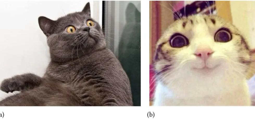
ANNs correspond to a computation technique using a network of simplified models to perform computations using learning processes. They are able to approximate any complex function by defining a training process where the network iteratively learns an association rule between a set of inputs and outputs. The network is built out of many simple parameterized computational units [13] whose value can be updated to continuously adjust the input to the correct output. They correspond to a model inspired by the biology of neurons (see fig. 2.2) , whose objective is to learn a potential mapping that occurs between inputs such as images (or text, audio, etc…) of, for instance, cats and provide outputs like: this is a cat.

We take advantage of an analogy to provide an intuition on the functioning of ANNs. When faced with a picture of a cat (fig. 2.1a), how do we know that this image corresponds to a cat? One possible reaction would be to respond that we know it because of the presence of features such as: fur, pointy ears, whiskers. The problem arises when we consider other images that challenge the assumptions built upon this choice of salient features. Say that one is confronted with an image in which the ears of the cat are occluded, as in fig. 2.1b. Now, how do we update our representation of the concept of cat? More simply: how do we still know that this is a cat? It does not seem likely that humans learn by having a complete database off all the features that make up each individual thing, from which we can deduce a simple equation such as fur+(ears+pointy) = cat. What seems to be the case is that we acquire information about entities based on examples that somehow relate to them, so when dealing with pictures of things like cats, we react with what we have learned in a sub-cognitive fashion and if we are asked how do we recognise a cat we delve into our internal representations and provide a cognitive expression of the potential constituents that make up the concept cat: it must have fur, it must have pointy ears and so on. On the next chapter we will illustrate some of the basic steps for building the mathematical foundation of artificial neural networks.

(17)

2. BACKGROUND

(a) (b)

Figure 2.1: Cats. On the left a cat where the salient features are visible (e.g. ears, whiskers). In panel (b) instead the absence of the ears makes the recognition of the cat more difficult. How do we still know that (b) is a cat?

(a) (b)

Figure 2.2: Biological and mathematical neuron. a. Image of a biological neuron with an axon, dendrites and a nucleus. b.Image of the basic computation of a neuron with the summation, addition of a bias value and an activation function.

2.2 The mathematics of Artificial Neural networks

The simplest unit of computation in an artificial neural network is the neuron. Each input that a neuron receives has a weight associated with it which represents the importance of that connection between that specific input and that unit. This neuron applies a nonlinear function to the weighted sum of its inputs. In symbols, we have

v=

n

∑

i=1

xiwi+ b

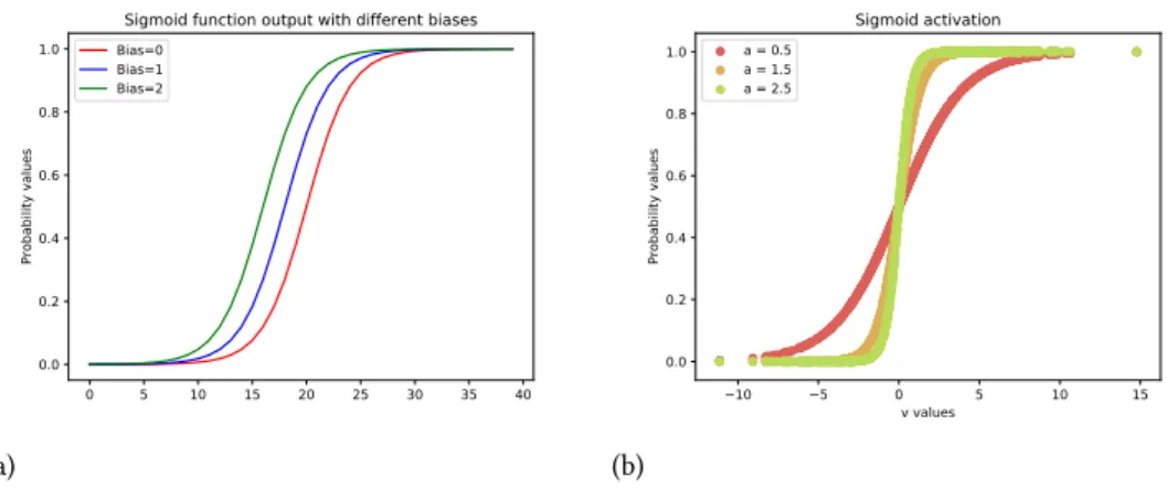
The b stands for the bias value: a learnable constant which serves as a threshold for the neuron’s activation and increases the model flexibility by shifting the boundary necessary for a neuron to activate (see fig. 2.3). But this value can be thought of as another weight that the network learns.

The main concept to be grasped here is that the synaptic strengths (in this case the weights w are learnable and control the degree of influence as well as its direction (excitatory is a positive weights and inhibitory is a negative weight) of one neuron over another. After the summation the final value passes through an activation function and its output is a value representing how active that particular neuron is, sending the information to the next neuron where the same computation will happen all the way to the end of the neural network, layer by layer. A common example for activation function is the sigmoid function,

f(x) = 1

1 + e−a(v) 4

(18)

2.2 The mathematics of Artificial Neural networks (a) 0 5 10 15 20 25 30 35 40 0.0 0.2 0.4 0.6 0.8 1.0 Probability values

Sigmoid function output with different biases

Bias=0 Bias=1 Bias=2 (b) 10 5 0 5 10 15 v values 0.0 0.2 0.4 0.6 0.8 1.0 Probability values Sigmoid activation a = 0.5 a = 1.5 a = 2.5

Figure 2.3: Understanding the role of different parameters. (a) The bias shifts the boundary necessary for a neuron to fire. (b) The constant value a affects the steepness of the curve, here we show the sigmoid output for the activation for three different values for the constant a

In this case the expression v represents the feed forward function with the multiplication of the input by the weights vector plus a bias. After that the output is fed to the sigmoid which squashes the value between 0 and 1.

Biologically the neurons are connected through synapses where information flows. When we train a neural network we want the neurons to be more active whenever they learn relevant patterns from the data, and we model this degree of influence using the activation function that squashes values between 0and 1 (in the case of a sigmoid) which represents how active that neuron is.

After this process is done and the input has passed through the entire neural network, an error value is computed for the output (for supervised learning models). This error corresponds to how far the output was from the real data. Usually there are two ways of computing an error: an unsupervised and a supervised way. The supervised way uses labels which correspond to the correct output value for a given input and they are usually assigned manually by the designer of the network. In the unsupervised setting, there are no labels and the model learns from the training data itself. There are many ways to calculate this error in both settings but the idea to keep in mind is that the error or cost function is a rule that teaches the network how far off it is from learning a correct representation of the data for a given problem. The error value computed will be propagated back to adjust the weights in order to minimize the output value of the error function. This process is known as backpropagation [50] and the most common algorithm to implement it is gradient descent [2].

Gradient descent is an algorithm that computes iteratively the partial derivative of the error func-tion with respect to each weight (the gradient), which corresponds to the right amount of adjustment that each weight needs to minimize the error function, meaning that it indicates the direction of steep-est descent in the landscape of this error function, taking it closer to a minimum, where the output error is low on average.

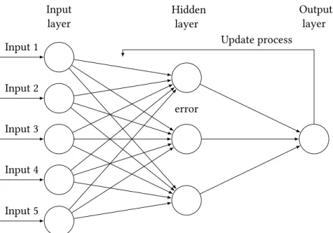
In summary: a neural network is a model defined in a layer-wise structure that is able to approxi-mate any complex function by optimizing a process of minimizing a pre-defined cost function. There are many types of networks from deep networks to shallow [37], convolutional networks [31], siamese networks [30] and many others, all of them subscribe to this basic architecture of layers, neurons and a learning cycle defined by this goal of minimizing an error function [37]. The goal of this section was to provide an overview of the basic concepts behind this process so that the explanations that will follow can tap into these intuitions and help our reader understand the methods implemented here to analyse

(19)

2. BACKGROUND

Input

layer Hiddenlayer Outputlayer

Input 1 Input 2 Input 3 Input 4 Input 5 error Update process

Figure 2.4: Schematics of the backpropagation algorithm in artificial neural networks. A summation function is applied to the inputs from the previous layers, followed by an activation function. An error is computed at the output layer and propagated back through an update process.

behavior.

2.3 Convolutional Neural Networks

CNNs (see fig. 2.5) are a type of neural network that resembles the connectivity patterns of neurons in the visual cortex [36]. It has been shown that individual neurons are spatially selective to specific regions of the stimuli known as the receptive field [25], these networks are able to successfully capture the spatial dependencies in an image through the application of relevant filters that represent this se-lectivity observed in neurons from the visual cortex. These types of networks have been shown to be a better fit to image datasets since these convolutional architectures make the explicit assumption that the input is an image that allows us them to encode certain properties into the architecture making the forward function more efficient (forward function refers to the process of the input passing from the input layers to the output layers in a neural network). In other words, the network can be trained to understand the diverse set of patterns with local dependency in an image better than regular neural networks [35, 32].

2.4 Generative Adversarial Networks

Generative Adversarial Networks GANs are a type of deep learning model architecture first in-troduced in [22] that tackles the problem of density estimation, meaning, the problem of finding an estimate based on observable data of an unobservable underlying probability density function. That can be translated into trying to find how likely it is that a given sample came from a given distribution [23]

The basic architecture of GANs is the following: two deep neural networks (usually fully connected networks or convolutional networks) are joined together on a competitive structure: one is called the

(20)

2.4 Generative Adversarial Networks

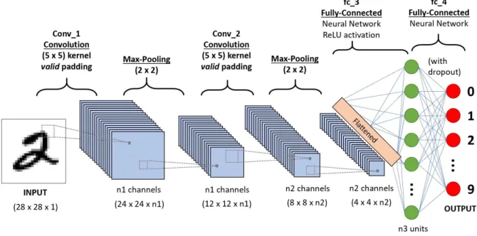
Figure 2.5: Convolutional network example to classify handwritten digits. On the left we see an example of the digit 2. It goes through, (in this particular example) two 5x5 kernels (or filters) and two max pooling layers (downsample stage of the convolutional network through the application of a fixed function that reduces the dimensionality of the input). After the last max pooling layer the input is flattened and then it goes through a fully connected layer (a normal neural network layer) where it gets turned into a probability of being a certain digit (multi-class classification). (This image was taken from [52])

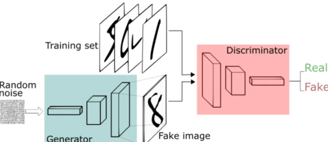
generator, and the other the discriminator. The generator iteratively attempts to capture the data distri-bution. Given a certain dataset of images for example (such as cats or handwritten digits) the generator takes as input a random vector and tries to produce images similar to them. On the other hand the discriminator estimates the probability that a sample came from the training data rather than from the generator (see fig. 2.6). In essence what GANs do is to learn a transformation of an input from a noise distribution (random values with the same shape as the input) to the training data [22]. The objective of the discriminator is, given a certain example from a distribution, to detect whether this example came from the generator’s distribution or from the real data distribution. A side-effect of the discriminator’s objective function is that as the generator gets better at producing fake samples, the discriminator will also get better at distinguishing between real and fake. The ultimate goal of this entire process is to have a generator that can confuse the discriminator so well that the discriminator outputs a 50% probability of that sample being real, meaning it can not distinguish between them (see fig. 2.7).

Usually the way generative models work is that they attempt to minimize an explicit density func-tion (such as PixelRNNs or Variafunc-tional Autoencoders) [46],now for GANS there is no explicit density function. They take a game-theoretic approach where both networks compete against each other in a 2-player minmax game [41], where the objective function of the generator is to minimize the log-probability of the discriminator being correct and the objective function of the discriminator is to max-imize its chances of being right [22].

(21)

2. BACKGROUND

Figure 2.6: Generative Adversarial Networks framework. The generator learns a transformation from the input noise vector to the real distribution of handwritten digits while the discriminator learns to separate the real data (actual handwritten digits) from the one generated by the generator (fake images of handwritten digits). This image was taken from [55]

Figure 2.7: Optimal learning for GANs. The dotted black lines represent the distribution of the real data, the continuous green line represents the distribution of the generator and the dashed blue line represents the discriminator. (a),(b),(c) Across epochs the generator approximates more and more to the real distribution to the point when we arrive at (d) where the discriminator is a flat line with 50% chance of separating between real and fake, meaning it can not successfully distinguish between both. This image was taken from [22]

2.5 Multi scale video prediction with Generative Adversarial

Networks (MVGANS)

Our goal was to quantify behavioral changes in mice during an experiment that involved some perturbation of the behavior baseline, an optimal model would be one that could represent internally the dynamics and content of the evolution of a video sequence. The model we used in this project was adapted from [42], where they present a model that offers a good approach to model the dynamics of video sequences. They took a multi-scale approach combined with an adversarial strategy to train convolutional networks to predict the future of frames given a certain limited past history. By doing that they were able to produce images of remarkable quality indicating that this might be a good path for unsupervised learning research.

The idea of video prediction refers to the problem of modelling video data, meaning how well can one predict the future of a certain video sequence given a certain number of past frames. It is a challenging problem because it involves high-dimensional natural-scene data with complex temporal dynamics [45], but it has been shown to be useful as a tool to model the dynamics of a sequence of images [42].

This type of model looks at a stack of a certain number of frames and tries to predict the entire frame 8

(22)

2.6 Serotonin

Figure 2.8: Prediction of future frames. On the extreme left the image represents the ground truth image from a clip of a man walking from left to right. On the right where the yellow tag is placed each box represents a prediction for what that ground truth image should be given an input of a history of past frames [3].

(a) (b)

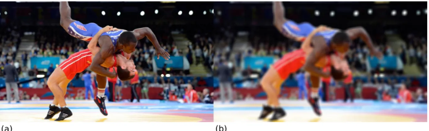
Figure 2.9: PSNR comparison. (a) Image with perfect psnr: 100. (b) Blurred image with a lower psnr value: 39.52

a certain interval in the future. By doing this iteratively it learns to represent the changing dynamics of the video sequences that it sees (see fig. 2.8). To evaluate the quality of the images produced by the generator, they used standard image quality metrics: the PSNR (peak signal to noise ratio) and sharpness difference between the gradient of ground truth images and the predictions. The PSNR is calculated as a ratio between the maxYˆ (the maximum possible value of pixel intensity in the predicted

image) and the mean squared error difference between ground truth image pixels and the pixels from the predictions. The equations for the both can be seen below.

PSNR(Y, ˆY) = 10 · log10·

max2_ˆ

Y

∑ni=1(Yi− ˆYi)2

Shar p.di f f .(Y, ˆY) = 10 · log10·

max2_ˆ

Y

∑i∑j|(|Yi j−Yi−1 j| + |Yi j−Yi j−1|) − (| ˆYi j− ˆYi−1 j| + | ˆYi j− ˆYi j−1|)|

2.6 Serotonin

Serotonin or as it is known in the neuroscientific community: 5-HT (5-hydroxytryptamine) is a major neuromodulator considered to be one of the most important pharmacological targets in the treat-ment of psychiatric disorders such as anxiety and depression [57]. A centered theory of 5-HT function has been elusive due to the the heterogenous nature of its known behavioral effects [16].

Serotonin is produced by a specific group of neurons found in an area at the base of the brain called the raphe nuclei. From there, serotonin is released into other parts of the brain to influence different behaviors (see section 2.6). Although drugs that target serotonin are widely used as antidepressants, how this chemical signal acts in the brain remains largely unknown.

(23)

2. BACKGROUND

(a) (b)

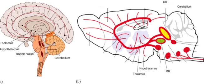
Figure 2.10: Schematics of the serotonergic system simplified (a) Here we give a simplified schematics of the main parts of the serotonergic system of a human brain. The raphe nuclei is the region of the brain responsible for the majority of the forebrains input of serotonin. It projects to the thalamus (located just above the brain stem between the cerebral cortex and the midbrain whose main function is to relay motor and sensory signals to the cerebral cortex). Also projects to the hypothalamus (located at the base of the brain it is responsible for many things such as control of the appetite and regulation of emotional responses), to the cerebellum (also located at the base of the brain it is responsible for coordinating voluntary movements) and to the spinal coord (a long, thin, tubular structure made up of nervous tissue, which extends through the vertebral column), (image adapted from [4]). (b) Here we see a similar schematics for the mouse brain. MR stands for median raphe and DR for dorsal raphe. There are many similarities between the serotonergic system in humans and mice and, the latter is usually used as a proxy to understand how the human serotonergic system works (image taken from) [38]

Serotonin modulation has a wide spread and diverse effect on behavior, e.g. it seems to affect the underlying factors that motivate actions [9] and to drive behavioral inhibition [12], [54]. This theory was motivated by data showing that 5HT depletion increases startle responses [15] and locomotor activity [21], [19] by altering the impact of the future motivating outcomes.

Given this complex landscape it is imperative that both the behavioral output and the tools we use to analyze the consequences of activating these specific neurons are rich and complex enough so that we can derive from them meaningful insights about the dynamics underlying the serotonergic system.

2.7 Related work

A recent study used optogenetics on serotonin-producing neurons in the dorsal raphe nucleus of mice [11] and found that by triggering serotonin production in the DRN (the major source of serotonin input to the forebrain) through phasic activation for a few seconds caused the mice to move around more slowly as they explored their surroundings. This short-term release of serotonin was found to be context dependent, meaning that the decrease in speed was only perceived when the mouse was spontaneously moving around a box without a clear goal such as finding water or balancing on a moving object. This context dependence was considered to be an indicator that serotonin was negatively affecting an individual’s motivation to move since they found nor motor (like impairment) or anxiety effect that could explain the decrease in speed. On the other hand, they also found that repeated daily phasic 5-HT activation of the DRN neurons resulted in a long-term enhancement of locomotion, which means, if those neurons were activated daily after a certain amount of time the mice got faster.

These findings seem to support the idea that serotonin causes some change in the behavior reper-toire that seems to be associated with motivation but does not describe what these changes look like.

(24)

What else can we detect? Is there any other read out from the behavior that could indicate serotonergic activation?

It would be interesting to see if there are other changes associated with stimulation but current methods to analyze the behavioral output of mice in open field are limited by factors such as the slow nature of manual annotation of behavior, its subjective and imprecise nature and its low dimensionality [1], [17]. On the other hand, in the last decade we have been watching a rise of automated approaches to behavioral analysis that seem to tackle a lot of the issues encountered in this field. Given the re-cent progress in machine learning models both in supervised and unsupervised settings [1], automated assessments of behavior seem to represent the future of how we understand behavior.

Attempts to characterize behavior in a unsupervised manner are not completely new. In [58] they tried to answer the question of what are the minimal components that underlie behavior and found a computational model that revealed structure in mouse behavior without observer bias. They saw that mouse behavior seems to be composed of stereotyped sub-second modules (behavior segments that last less than one second) with defined transition probabilities that arrange themselves to form big and semantically meaningful behaviors. They performed an unsupervised analysis to reveal how genes and neural activity impact behavior and concluded that these identifiable components were organized in a predictable fashion. The framework proposed could be useful to unravel the influence of environmental cues, genes and neural activity on behavior. In a following paper (by the same lab), it was discovered that this modularity of behavior might be encoded in the dorsolateral-striatum and that this region seems to flexibly assemble behavioral sequences from sub-second components [40]. These discoveries point to unsupervised learning as a powerful tool to describe behavior given that impressive range of their results although their approach had assumptions that make the model not completely unsupervised. However they did not provide tools to quantify activation of subset of neurons that might cause change in behavior, so although the framework is extremely rich it does not provide a clear path to quantify how different regions of the brain affect behavior in comparison to a learned baseline. In our work we would like to extend the literature by providing a method based on GANs to quantify this distinction between baseline and non-baseline behavior allowing for unsupervised detection of brain specific stimulation from analysis of raw video of behaving mice.

(25)

(26)

Chapter 3

Methods

In this chapter we will give a detailed description of all the procedures and algorithms utilized in this project. As a disclaimer we must note that the capsule network model and the generative model were already implemented by researcher Mattia Bergomi upon the arrival of the author of this thesis in the Champalimaud Foundation. The contributions of this thesis are not on the realm of introducing novel machine learning architectures but on its usage for behavior analysis as well as developing the pipeline for integration of the algorithms along with writing a graphic user interface, performing the data analysis and writing custom algorithms to deal with problems related to the alignment of the pose of the mice that will be detailed below. Also, helper functions were written to aid the already implemented models to perform tasks such as fine-tuning of the segmentation model, training and testing of the generative model and others. The main contributions and procedures developed within the context of this thesis will be detailed below.

On the first section of this chapter we will discuss the dataset and inform the reader about the protocol of stimulation and the source of the dataset for context fig. 3.1. In the second section we will discuss the problem of segmenting the mice in the open-field arena where they were recorded fig. 3.3, along with a description of the challenge of segmenting mice in such conditions we describe the graphic user interface developed in the python programming language to aid on the preprocessing of the videos as well as their segmentation. Together with this explanation we will demonstrate the need for the architecture used and we will provide an intuition for why it was relevant to this specific problem. On the third we define the pipeline of the unsupervised detection of the mice as well as our assumptions about predictability and the model used, its loss function, training procedure and relevance for the problem of analysing behavior. In the fourth section we show how we produced videos of mice where their pose was aligned with the north-east corner of the frame to investigate if the detection was still possible, even in situations where there was no displacement speed; we also demonstrate why this was a relevant problem to pursue. On the last section of this chapter we will give a brief list of all the frameworks used for the execution of this project. A diagram of the entire pipeline for this project can be seen here fig. 3.7.

3.1 The dataset

The dataset we used was provided to us by [11]. It is composed of videos of mice moving around in the open field arena, a widely used assay to study locomotion and anxiety-like behavior ([53]). The mice were subjected to a protocol of optogenetic activation of their serotonergic neurons located in the dorsal raphe nuclei to assess the behavioral effect of this neuromodulator in the spontaneous behavior

(27)

3. METHODS

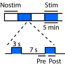
Figure 3.1: Stimulation protocol. Videos of average 30 minutes were divided in blocks of 5 minutes that alternated between stimulated block and non-stimulated block. Both blocks were divided in trials of 10 seconds, of which, during stimulated blocks, the protocol of activation of the neurons with a light stimulus was 3 seconds light on and 7 seconds light off. During non-stimulated blocks there was no activation but the division in trials of 10 seconds was kept to allow for comparison. This image was taken from [11].

of the mouse. We would like to give a quick explanation of their protocol of stimulation to provide context for the analysis that we did using the same dataset.

The protocol of stimulation

The experiment lasted on average 30 minutes although a few videos were longer up to 45 minutes. The videos were divided into blocks of 5 minutes where during each block the mouse was either being stimulated or not being stimulated (fig. 3.1). Every video began with a non-stimulation block and then it would alternate between stimulated and not stimulated. While in a stimulation block, the period where the mouse was actively receiving a light stimulus that activated the serotonergic neurons lasted 3 seconds followed by a 7 seconds of no light and repeat till the end of the 5 minutes block. What we called trials in this thesis refers to this 10 seconds period of 3 seconds light on and 7 seconds light off, and during the non-stimulation period the trials were divided in the same manner but there was no activation with the light. To understand better this process of activation through a light stimulus (a technique formally known as optogenetics) see [59].

3.2 Capsule Networks for segmentation

Why Capsule Networks?

To be able to run our model on images of freely moving mice, we segmented the frames of the videos in order to subtract the background from the foreground of the images (in our case we wanted a video of only the mouse moving around without any other interference).

Object segmentation is a difficult problem. The task itself can be described as the combination of two problems: object recognition and object delineation. On the object recognition side, the objective is to locate the presence of an object inside of an image. On the delineation part, the challenge is to draw the object’s spatial extent and composition. Solving these two problems together results in the separation of foreground (the intended object to segment) and the background (everything else) [33].

(28)

3.3 Unsupervised detection of non-baseline behavior with MVGANs

Early attempts in automated object segmentation relied on rule based systems where a complex sys-tem of rules were defined to teach a machine to automatically distinguish foreground from background. Over the last few years, deep learning based methods particularly convolutional neural networks [35] became the state of the art in all sorts of tasks related to image analysis including segmentation [48].

However, the computational units on CNNs are ambivalent to the spatial relationships of the units within their filter of the previous layer and, therefore, within their effective receptive field of the given input [33]. Recently, a new architecture has been introduced to the public: capsule networks. In these networks [51] information is stored as vectors rather than scalars as it is the case of CNNs. Within these vectors there is information concerning: spatial orientation, magnitude/prevalence and other attributes of the extracted features. All of this information is stored into what the authors called capsules which are routed to capsules in the next layer via an algorithm that takes into account the agreement between these capsule vectors. This architecture allows these capsules to form meaningful part-to-whole relationships not found in a standard CNN. [33].

Implementation

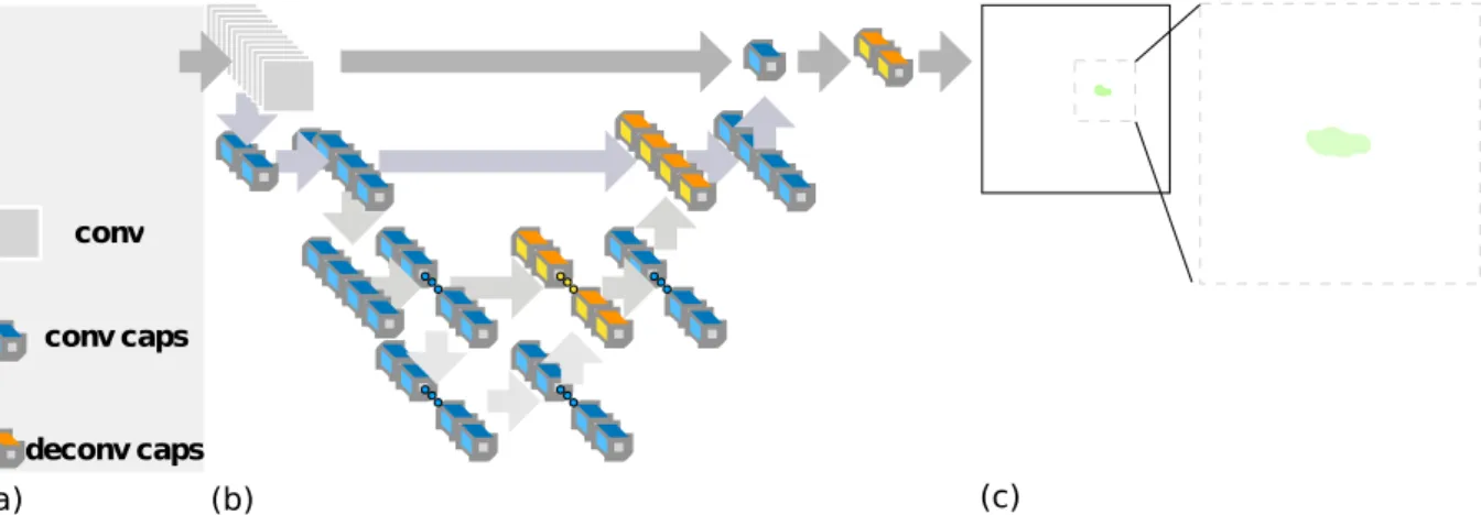
A mouse implanted with an optogenetic drive, its color, bedding and implant make it impossible to segment this image with standard thresholding techniques. Background subtraction is minimally effective, given the stereotypical locomotion of a mouse (when freezing or resting the mouse would be subtracted). At the same time, relying on optic flow would not be robust to occlusion. To solve this problem, we adapted the SegCaps network [33], a capsule network [51] version of Unet [48] for the analysis of 2-dimensional images. The model was trained on a dataset of natural images and fine-tuned to our dataset of images of mice moving around the open field. Convolution and deconvolution capsule layers learn equivariant relationships with respect to complex transformations of the input. That means that the model can build a representation of the input that encompasses part-to-whole features like the body part relationships of a mouse. The enhanced generalization power of capsule networks enables segmentation of complex images without relying on optic flow analysis or dynamical constraints. Graphic user interface for thresholding and segmentation

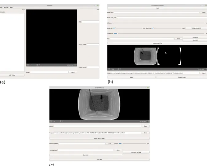
To use the model effectively we developed a user friendly interface to interact with it as well as perform preprocessing on the frames of the videos. For that we developed a customized graphic user interface to facilitate these processes fig. 3.2. The functionalities of the GUI involve:

• Basic thresholding • Basic blob extraction

• Direct interaction with the segmentation model for segmenting entire videos • Fine-tuning of the model to improve performance on novel datasets.

3.3 Unsupervised detection of non-baseline behavior with MVGANs

Our general goal was to learn a behavioral baseline, in an unsupervised fashion, in order to detect relevant fluctuations from such baseline. To do that we developed a deep-learning-based method for quantifying fluctuations in behavior with respect to a learned baseline fig. 3.4. Both spatial and temporal

(29)

3. METHODS

(a) (b)

(c)

Figure 3.2: Graphic user interface for preprocessing and segmentation. (a) Initial window where the video can be loaded and some information is provided like frame rate and the videos’s resolution. (b) Preprocessing window where thresholding, dilation, blob extraction can be performed on the entire video. Also a mask generation option is offered where the user can produce a dataset of masks of the current frame to fine-tune the segmentation model. (c) A segmentation window where the user can interact with the segmentation model to segment entire videos. If the results are not optimal the user has an option of fine-tunning the model to their dataset.

organization of events are taken into account in learning baseline behavior, and then are used to assess the predictability of new events. We applied it to raw behavioral videos of mice moving around the open-field arena to test if we could detect the behavioral effect of serotonergic stimulation. Before we go further with the explanation of the pipeline we must define briefly what we mean when we use the term predictability.

Predictability

By predictability we mean the degree to which a correct prediction can be made about the future of a certain system’s state[7]. In our case we consider predictability to be a meaningful feature of behavior itself and we defined a metric (fig. 2.9) that enabled us to quantify how predictable a certain configuration of the entire body of the mouse was. With this information we investigated if we could acquire insight about the behavior by assessing the fluctuation of this metric during baseline behavior (non-stimulated) and non-baseline behavior (stimulated), where a higher value corresponds to a more predictable configuration and vice-versa.

(30)

(a) (b) (c)

conv conv caps deconv caps

Figure 3.3: Segmentation with Capsule Networks. Segmentation of a video frame of a mouse in the open field. (a) Input: A mouse implanted with an optogenetic drive moving around in the open field arena. (b) Pre-trained 2D SegCaps: The architecture of the SegCaps network [33]. (c) Output of the model, after training on segmentation of natural images and light thresholding to eliminate small blobs.

Experiment procedure

We considered videos of mice in open-field receiving optogenetic activation of dorsal raphe sero-tonin neurons (see fig. 3.1). First, we applied a semi-supervised segmentation method using capsule networks [33] to remove the noise produced by the background and fiber optic cable (see fig. 3.3). Afterwards, multi-scale video prediction generative adversarial networks (MVGAN) [42] were used to learn a behavioral baseline directly from non-stimulated video segments. The network architecture can be found in 3.1 and although the explanation of the algorithm can be found in [42] we will also provide it here to strengthen the understanding of our approach.

The model

As stated in [42], consider two sequences Y and X where Y = Y,...,Yn _{and X = X,....,X}n_{. Y is}

the sequence of frames to be predicted from input X. A network G is trained to predict one or many concatenated frames Y by minimizing a distance lp(where p = 1 or p = 2) between the predicted frame

and the true frame,

Lp(X ,Y ) = lp(G(X ),Y ) = ||G(X ) −Y ||pp (3.1)

The problem is that a network trained like this would face two problems: loss of resolution due to the fact that convolutions (the process performed by filters in a convolutional network to learn features from the images) only accounts for short-range dependencies that are limited by the size of the filters. The second problem is that using l1 and l2 usually yields blurry results. Imagine that the probability

distribution for an output pixel has two equally likely possibilities, the value that would minimize l2

would be the average between both even if this value has a very low probability on the distribution. In the case of l1would be the median but still the results would be too blurry.

To tackle these problems the authors in [42] proposed two strategies: a multi-scale network and the adversarial training.

(31)

3. METHODS

The multi-scale network

Instead of making G predict over only one resolution of the input (the standard way to train gen-erative models based on convolutional networks) the authors proposed a multi-scale architecture. Let s₁, ..., snbe the sizes of the inputs to the network. Let uk be an upscaling operator toward size sk (we

used four sizes [4,8,16,32]). And let Xi k, Y

i

k denote the downscaled versions of X

i_{and Y}i_{of size s} kand

G0be a network that learns to predict Yk− uk(Yk−1)from Xkand a guess of Yk. A network Gkis defined

that makes a prediction ˆYkof size sk,

ˆ

Yk= Gk(X ) = uk( ˆYk−1) + G0k(Xk, uk( ˆYk−1)). (3.2)

With this the networks makes a series of predictions, starting from the lowest resolution and using the prediction of size sk as a starting point to make the prediction of size sk+1. In the beginning of

training the network takes only X1as input. The network architecture is shown in 3.1. The weights are

denoted by WGand the minimization in our case is performed with the Adam optimizer [29]. In [42]

they used stochastic gradient descent but in our case we found this optimizer to be more effective. Adversarial training

Although in [42] was found that the multi-scale network helped reducing the blurriness of the future predictions, the results were still too blurry. In our case having blurry results would be even worst given that predicting a blurry configuration of the mouse would not tell us much about the behavior. To solve that, the authors proposed an adversarial strategy [22]. Now G is trained simultaneously with a discriminator D (both models are based on convolutional networks ([35]), to acquire an intuition for how these networks work see 2.3). The generative model G takes as input a sequence of frames and is trained to output a prediction for the future of that sequence a certain number of frames ahead, meaning it learns to generate a prediction for what the entire future frame of that sequence would look like. The discriminative model D takes as input a sequence of frames, and is trained to predict the probability that the last frames (Yn_{) of that sequence is generated by G. Remembering that only these last frames}

are either generated by G or real frames from the video. With this procedure the discriminative model is able to leverage temporal information and therefore G learns to produce images that are temporally coherent with its input.

This strategy addresses the problem of predicting averages of possibilities as we stated before. Us-ing an adversarial strategy when we have a sequence (X,Yavg), D will be able to discriminate them

easily. The only pairs of images D will not be able to discriminate easily are sequences that have equal probability, therefore, the generator will learn how to approximate the distribution that resembles the distribution of possible future frames Y.

Dis trained to classify the input (Xk,Yk)as 1 (a sequence of frames and a real frame), and to classify

(Xk, Gk(X ))as 0, where k is the scale of the input, for which we perform one iteration of the Adam

optimizer over Dk while keeping the weights of the generator fixed. The loss function used to train D

is: LD_adv(X ,Y ) = Nscales

∑

k=1 Lbce(Dk(Xk,Yk), 1) + Lbce(Dk(Xk, Gk(X )), 0) (3.3) 18

(32)

Lbceis the binary-cross-entropy loss, defined as

Lbce(Y, ˆY) = −

∑

i

Yilog(Yi) + (1 − ˆYi)log(1 −Yi) (3.4)

where Yi takes values in {0,1} (can be either 0 or 1) and ˆYi takes values in [0,1] (can be any values

within 0 and 1.

To train G we keep the weights of D fixed and perform one optimization step with Adam to minimize an adversarial loss, LG_adv(X ,Y ) = Nscales

∑

k=1 Lbce(Dk(Xk, Gk(Xk)), 1) (3.5)

Minimizing this adversarial loss means that G is attempting to confuse D as much as possible so that Dwill not be able to discriminate predictions correctly. The problem here is that this does not guarantee that G will learn to generate images that are similar to Y because it can always produce confusing samples without them being closer to Y. To fix this problem in [42] was introduced a composition of the adversarial loss and the Lploss described earlier. G now is trained to minimize λadvLG_adv+ λlpLp. By having to minimize this, the model has a tradeoff to adjust by the mean of the parameters λadv

and λlp. From the first term similarity based on sharp predictions given the adversarial principle and similarity with the real image enforced by the second term that minimizes an lploss. A description of

the algorithm can be found in Algorithm 1. Set the learning rates pDand pG, λadvand λlp while not converged do

Update the discriminator D

Get M data samples (X,Y) = (X1_,Y1_{), ..., (X}M_,YM₎

WD= WD− pD∑Mi=1

∂ LDadv(Xi,Yi)

∂WD Update the generator G

Get M new data samples (X,Y) = (X1_,Y1_{), ..., (X}M_,YM₎

WG= WG− pG∑Mi=1(λadv ∂ LG_adv(Xi_,Yi₎ ∂WG + λlp ∂ LG_lp(Xi_,Yi₎ ∂WG ) end

Algorithm 1:Training adversarial networks for next frame generation

Another strategy introduced by [42] to sharpen the image prediction is penalizing the differences in the gradients of the predictions in the generative loss function. With this they defined a novel loss called Gradient Difference Loss (GDL) that can be combined with the other mentioned losses here to produce better results. This function between the ground truth and the prediction can be defined as,

Lgdl( ˆY,Y ) =

∑

i j

||Y_{i, j}−Y_{i−1, j}| − | ˆY_{i, j}− ˆY_{i−1, j}||α_{+ ||Y}

i, j−1−Yi, j| − | ˆYi, j−1− ˆYi, j||α, (3.6)

here, α is an integer value greater or equal to 1 and |.| represents the absolute value function. This loss penalises gradient differences between the prediction and the true output by considering the neighbor pixel intensities differences.

The final loss we used (as the authors in [42]) combines all of the above on a final expression, L(X ,Y ) = λadvLGadv(X ,Y ) + λlpLp(X ,Y ) + λgdlLgdl(X ,Y ) (3.7) We trained the model on non-stimulated blocks of the videos and tested in both blocks of stimulated and non-stimulated (we always left one block of non-stimulated for testing). We used stacks of 10

(33)

3. METHODS (a) Generator Discriminator Legend input multiscale conv non-linearity max-pooling latent space upsampling conv softmax real fake (b) (c) (d) PSNR Trial duration (e) PSNR Trial duration

Figure 3.4: Pipeline overview for unsupervised detection. (a),(b) Segmentation with capsule networks of freely moving mice in the open field arena.(c) Application of multi-scale generative adversarial networks model. (d) Analyses of the fluc-tuations of the PSNR and sharpness of stimulated (gold) and non-stimulated (green) portions of the video. (e) We applied k-means algorithm (k = 2) fig. 3.5 to define an unsupervised threshold for stimulation (the red portion of the fluctuation means the unsupervised detection of the stimulated mice) computed as the mean of the centroids found.

frames as input and predicted for three intervalsthe problem is that in the future: 5, 10, and 15 in individual videos. The best results were found with an interval of 10 which is the protocol used on the entire dataset along with minibatches of 1.

DISCLAIMER.The description of the above algorithm was taken from [42] in its almost entirety and shown here with the purpose of providing an explanation for the computations behind our model and our calculation of the predictability index. It does not represent an original contribution of this thesis, nor was it implemented by the author of this thesis. The work described here was to use and adapt this architecture to fit our problems which involved minor issues of fitting and adapting to our dataset as well as apply it to obtain the results with which we performed the detection.

PSNR and sharpness as predictability indexes

When we test the model (trained on portions of the video where the mouse was not stimulated) on both non-stimulated and stimulated portions of the video, the quality of the predictions measured in the PSNR and sharpness provided what we call a predictability index. This index means that higher values indicate that the future of that particular portion of the video was more predictable, and were used to explore the deviation from baseline. The trends of these metrics in stimulated and non-stimulated

(34)

Generative network scales G1 G2 G3 G4

Number of features maps 128,256,128 128,256,128 128,256,512,256,128 128,256,512,256,128

Conv. kernel size 3,3,3,3 5,3,3,5 5,3,3,3,5 7,5,5,5,5,7

Adversarial Network scales D₁ D₂ D₃ D₄

Number of features maps 64 64,128,128 128,256,256 128,256,512,128

Conv. kernel size (no padding) 3 3,3,3 5,5,5 7,7,5,5

Fully connected 512,256 1024,512 1024,512 1024,512

Table 3.1: MVGANs architecture Four generators and four discriminators are outlined here because the network uses a multi-scale architecture and the input passes through the network four times at increasingly bigger scales. For more details see [42]

One dimensional values of PSNR

Kmeans for detection

Non-detected values Detected values Threshold of detection

Figure 3.5: Kmeans detection example.The threshold value is calculated as the mean between the two centroids found. The input to the kmeans is the entire dataset of PSNR for all videos averaging across trials including both stimulated and non-stimulated moments. The example shown here is just to clarify the concept and does not involve real data.

segments were used to detect the effect of the serotonergic stimulation, and quantify this effect. As explained in section 2.5 the PSNR and sharpness are metrics for comparing images. In our case the model predicts an image given a stack of past frames and, the quality of this image according to the referred metrics is considered to represent how predictable that image was given that input. So through out the course of this thesis we will refer to the fluctuations of the PSNR and sharpness as the predictability indexes of the mouse, given that the images the model is predicting are solely composed of the mouse configuration segmented from the background.

Using k-means to acquire a threshold for detection

We used the k-means algorithm (k = 2) [26] on the one-dimensional fluctuation of PSNR (for sim-plicity we only show PSNR but sharpness gave similar results) to set a threshold for what would be considered the frontier between detected non-baseline behavior and non-detected behavior. A scalar value that separates what was detected from what was not (see fig. 3.5). This threshold is calculated as the mean of the two centroids found with the kmeans.

(35)

3.4 Pose alignment procedure

We also applied the model in a processed version of the same videos where the bodies of the mice were aligned with the north-east corner of the frame so that we could capture only variations in the pose (postural movement). We did this to assess whether our detection of the stimulation effect on behavior was over-reliant on the displacement speed of the mouse, meaning, maybe we were capturing only variations related to speed of the mouse moving around the box and not more granular information related to the difference in the body postures. By doing this analyses we could investigate if there were changes in posture closely related with the stimulation by evaluating whether the predictability of the configuration of the poses of the mouse would change according to the stimulation.

Protocol

First, we tracked the mouse by tracking the location of the centroid of the frame after thresholding our segmented videos. This thresholding worked well because the segmentation had already excluded all the undesired information (see fig. 3.3). We used the coordinates of this centroid obtained from our tracking to crop a bounding box of 256X256 pixels around the mouse in the original video to acquire a high-resolution video of the mouse moving around where the animal is always in the center of the frame. We segmented this cropped video to eliminate the same problems with the original. Then, at each frame, we tracked the head of the mouse using deeplabcut [43]. We applied principal component analysis [28] to the entire image to acquire an axis corresponding to the orientation of the mouse and we aligned the mouse with the north-east corner of the frame by rotating the entire frame to coincide with the alignment of the mouse’s axis. We used the coordinates obtained from the tracking of the head to make sure that when the PCA gave the wrong axis (because the mouse was in a stationary position for example and it confused the correct orientation) we could make sure that it would continue aligned correctly. By taking into account the orientation we assure that the head of the mouse is always pointing to the north-east corner. We finally generated videos of the mouse where the only changing factor in the frames corresponded to postural movements of the mouse without any displacement or rotation (see fig. 3.6).

3.5 Frameworks

For the completion of this project we used only the python programming language for the data analysis, GUI development and all of the programming tasks required. A gitlab link with the source code will be provided to the examiners of this thesis but could not be disclosed here due to the fact that this is still unpublished material.

(36)

3.5 Frameworks

(a) (b)

(d) (c)

Figure 3.6: Pipeline pose alignment. (a), (b) We obtained the coordinates from the centroid of the mouse in the freely moving videos and cropped a square of 256X256 pixels around it. (c) We segmented this cropped video (d) We aligned the pose of the mouse with the north-east corner.

(37)

3. METHODS Input / output Process Legend K-means MVGANs detection _S.3.2sec PSNR ﬂucutation Sharpness ﬂucutation S.3.2 sec Segmentation raw video Pose alignment video (pose aligned) Segmentation S.3.1 sec segmented video segmented video light thresholding thresholded video S.3.3 sec scalar value (threshold for detection) unsupervised detection

PSNR ﬂucutation with non-baseline behavior detected

Sharpness ﬂucutation with non-baseline behavior detected

S.3.2

sec

Figure 3.7: Pipeline diagram for the entire project. In this diagram we present an overview of the entire process, the white boxes on the corner refer to the sections where the reader can find detailed information about the procedure referred in the box. Light blue boxes represent the input or output from a given process and dark blue boxes represent the process being done.

An unsupervised generative strategy for detection and characterization of rare behavioural events in mice in open fiel to assess effect of optogenetic activation of serotonergic neurons in the dorsal raphe nuclei

University of Lisbon, Champalimaud Institute

Lucas B. Nicolosi Soares