Agrometeorological models for estimating sweet cassava yield
1Victor Brunini Moreto2, Lucas Eduardo de Oliveira Aparecido3,
Glauco de Souza Rolim2, José Reinaldo da Silva Cabral de Moraes2
INTRODUCTION
One of the three main human food sources in the world, besides rice and maize, roots of cassava (Manihot esculenta Crantz) present a high nutritional value and are considered an important food complement, playing a fundamental role for food security in tropical regions, which are mainly represented by developing countries (FAO 2012, Gabriel et al. 2014).
Cassava is a Brazilian native plant that belongs to the Euphorbiaceae family, and it is a valuable crop, mainly for the economies of countries in development, due to the versatility of in natura and
ABSTRACT
RESUMO
industrialized sub-products and by-products (Zanetti et al. 2014).
Brazil is the fourth largest producer of cassava in the world, after Nigeria, Thailand and Indonesia. In the growing season of 2016, 23.71 million tons of cassava roots were harvested. Currently, the Pará state leads the cassava production in Brazil, followed by Paraná and Bahia (Conab 2017). The southeast region is responsible for 11 % of all the cassava produced in the country, being São Paulo the most productive state, with about 1.4 million tons of cassava per year. Nevertheless, the production of the São Paulo state has been decreasing during the past few years. With respect to production, São Paulo stands out due to its
1. Manuscript received in Nov./2017 and accepted for publication in Mar./2018 (http://dx.doi.org/10.1590/1983-40632018v4850451). 2. Universidade Estadual Paulista, Faculdade de Ciências Agrárias e Veterinárias, Departamento de Ciências Exatas, São Paulo,
SP, Brasil. E-mails: [email protected], [email protected], [email protected]. 3. Instituto Federal de Educação, Ciência e Tecnologia de Mato Grosso do Sul, Naviraí, MS, Brasil. Brazil is the fourth largest producer of cassava in the
world, with climate conditions being the main factor regulating its production. This study aimed to develop agrometeorological models to estimate the sweet cassava yield for the São Paulo state, as well as to identify which climatic variables have more influence on yield. The models were built with multiple linear regression and classified by the following statistical indexes: lower mean absolute percentage error, higher adjusted determination coefficient and significance (p-value < 0.05). It was observed that the mean air temperature has a great influence on the sweet cassava yield during the whole cycle for all regions in the state. Water deficit and soil water storage were the most influential variables at the beginning and final stages. The models accuracy ranged in 3.11 %, 6.40 %, 6.77 % and 7.15 %, respectively for Registro, Mogi Mirim, Assis and Jaboticabal.
KEYWORDS: Manihot esculenta;crop modeling; climatology.
Modelos agrometeorológicos para estimar o rendimento de mandioca doce
great average yield (23.59 t ha-1), while in the Pará
state the average yield is 14.62 t ha-1 (IBGE 2016). In
the São Paulo state, 13 % of the cassava production areas are devoted to sweet cassava (Valle & Lorenzi 2014).
The most influential factors that affect the
sweet cassava quality are the genetic composition of the cultivar (Valle et al. 2004) and the environmental conditions. The sweet cassava quality is determined by various factors, especially low cyanogenic levels and low acid content, which reduce the risk of poisoning by cyanide, a highly toxic chemical substance (Mezzete et al. 2009).
Establishing relations between plant phenology and environmental conditions (for example, air
temperature and soil moisture) will aid in defining
technical agronomic criteria for cassava crops, such as planting spacing and mechanization (Rós et al. 2011).
Few studies have analyzed the influence of climate effects on cassava crops. Lahai et al. (1999) observed different responses of cassava development and production under different conditions of sunshine
hours, air temperature and rainfall. Cassava is tolerant to conditions of long dry periods and high precipitation; however, it is necessary to manage soil drainage conditions. Soils with poor drainage are susceptible to waterlogging, what may lead to root rot and substantial losses in yield (Tremacoldi 2016). Normally cultivated on low fertility soils, and
adaptable to climate variability, cassava is considered as the main example of a sustainable food of the 21th century (Valle et al. 2007).
Air temperatures between 25 ºC and 29 ºC and annual rain averages between 1,000 and 1,500 mm are considered optimal conditions for cassava development. Commonly cultivated under rainfed systems, rain events are the most limiting factors for its production (Alves 2006).
Agrometeorological models are helpful tools for decision makers about agricultural activities. Incorporating climate information to the crop
production allows the demonstration of its influence
during the crop cycle. In addition, this information is used to develop estimation models for crop quality and yield (Moreto & Rolim 2015).
This research aimed at the development of agrometeorological models to estimate the annual yield of sweet cassava for the São Paulo state, as well
as to identify and describe the influence of climate
during the crop cycle.
MATERIAL AND METHODS
The climatic data of the producing regions (Figure 1) were provided by the Instituto Agronômico de Campinas, in Campinas, São Paulo state, Brazil. These regions correspond to 80.3 % of the total cassava production in the São Paulo state (São
Paulo 2008). Monthly precipitation and mean air temperature from 1999 to 2014 were used to calculate the potential evapotranspiration, using the Thornthwaite (1948) method (equations 1, 2, 3, 4 and 5). This method, even though it is not the most indicated for São Paulo, is the one with the highest accuracy, when using a database that is limited in terms of climatic variables (Caporusso & Rolim 2015):
PET = ETp x COR (1)
{
ETp = 16 x(
10 x Tn)
a, if 0 ≤ Tm < 26.5 ºCI
ETp = -415.85 + 32.24 x Tm - 0.43Tm2, if Tm ≥ 26.5 ºC
(2)
I =
∑
12 (0.2 x Tn)1.514n = 1 (3)
a = 0.49239 + 1.7912 x 10⁻² x I - 7.71 x 10⁻⁵ x I2 + 6.75 x 10⁻⁷ x I3 (4)
COR = N x NDP
12 30 (5)
where PET is the potential evapotranspiration (mm month-1); ETp the standard evapotranspiration;
COR the correction factor, in function of the actual number of days and the photoperiod of the month; Tm the mean air temperature of the month n; I the index that expresses the heat level of the region; a the regional thermal index; NDP the number of days of the period; and N the mean photoperiod of the month.
The potential evapotranspiration was used in the sequential water balance model (Thornthwaite & Mather 1955) to generate information of monthly
water deficit, water excess and soil water storage,
using the available water capacity (AWC) of 100 mm (equation 6). For soil texture, loamy soils for all regions and an average cassava crop root depth
of 50.0 cm (FAO 2013) were used. According to Doorenbos & Kassam (1994), to create a practical criteria, the average available water capacity for clay and loamy soils can be estimated as 2.0 mm cm-1:
AWC = AWC x Zr (6)
where AWC is the average available water capacity (mm cm-1) and Zr the average cassava root depth
(cm). The annual yield data for sweet cassava were obtained from the lnstituto de Economia Agrícola, in São Paulo, for the period of 1998 to 2014.
The use of multiple linear regression requires the selection and combination of independent
variables for the development of significant models.
For this step, the method proposed by Walpole et al. (2012), which tests all possible combinations between the pre-selected independent variables, was used in the analysis.
T h e i n d e p e n d e n t v a r i a b l e s m e a n a i r
temperature, precipitation, water deficit, water excess
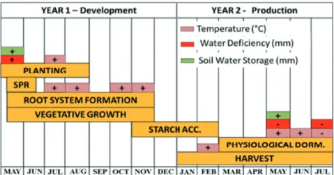
and soil water storage were used to develop the models with multiple linear regression (equation 7). A period of 10 to 12 years was used for calibration and 4 years for testing. As cassava has a cycle of up to 15 months (Figure 2), 15 monthly datasets were used for each meteorological variable, totaling (5 x 15) = 75 possible independent variables to use in the models for each location:
Y = a x X1 + b x X2 + c x X3 + … + LC (7)
where Y is the yield, in t ha-1; a, b, c,… the
angular coefficients; X1, X2, X3,… the selected monthly meteorological variables; and LC the linear
coefficient.
Models with up to 3 Xn in the equation were tested, totaling 156,348 possible equations
for estimating the sweet cassava annual yield. All monthly meteorological variables may have a relative importance for the crop development and production, but we searched for the most important ones. The
selection was based on coefficients of significance to select the variables (t < 0.05) and regressions (F < 0.05), as well as the minimization of the mean
absolute percentage error (MAPE) and maximization of the adjusted R² (equations 8 and 9):
N
MAPE (%) =
∑
i = 1(|
Yesti - Yobsi
|
x 100)
Yobsi
N (8)
Adjusted R2 =
[
1 - (1 - R2) x (N - 1)
]
N - k - 1 (9)
where Yesti is the estimated yield at the year i; Yobsi the observed yield; N the number of data; and k the number of independent variables in the regression.
For evaluating the angular coefficients of the Xs of the models, an analysis was conducted to remove the multicollinearity between the Xs (mean
air temperature, precipitation, water deficit, water
excess and soil water storage). Multicollinearity is not an issue when the interest is just estimation.
However, if the analysis of the angular coefficients of
the variables is also conducted, multicollinearity may
cause bias in these coefficients by not expressing the influence of these variables on the model (Gujarati &
Porter 2011).
RESULTS AND DISCUSSION
Among the regions with the highest production in the São Paulo state, climate variability is responsible for the widest range of variation in yield. Comparing the Registro and Jaboticabal regions, these present a similar average yield (14.0 t ha-1),
but Registro has a slightly higher accumulated water
deficiency (more than 100 mm), which may decrease
yield, and the inverse occurs for Jaboticabal, where,
even in seasons with a high water deficiency level,
yield is maintained above the average. In Assis and Mogi Mirim, the average yield is 18 t ha-1, and the
variability among seasons did not follow a pattern, with dry and wet seasons presenting both high and low yields, what indicates that the timing and extension of these periods (dry and/or wet) during the
crop cycles could influence the final yield (Figure 3).
For each region, about 57,000 model combinations were generated. Subsequently, the combinations that presented multicollinearity between the independent variables were removed. For the Jaboticabal region, 5,441 equations demonstrated multicollinearity, while the remaining ones (51,784) represent the possible models to estimate sweet cassava yield. From these models, the better ones
were selected and classified looking for a low mean
absolute percentage error, adjusted R2 near 1 and p < 0.05.
Based on the viable models, the five best ranked (Table 1) were selected, following the criteria
of significant models (p-value < 0.05), lowest mean
absolute percentage error and adjusted R² closest to 1.00 for the tests (validation).
Empirical models are based purely on quantitative interactions between the observed variables considered. These modeling methods are normally derived from regression analysis and are highly dependent on databases with ample data,
and long data series may be sufficient to achieve an
accurate response of a situation (Corrêa et al. 2011). A series of 15 years of data was used to develop the models and, even though the availability of cassava production data was scarce, it was still possible to
achieve accurate models for the specific productive
regions of the São Paulo state. In general, the models presented a good accuracy, with mean absolute percentage error values ranging from the best [3.11 % (Registro)] to the worst [18.72 % (Assis)], in the tests. For example, if we consider an average yield (15 years) of 14.42 t ha-1 for Registro, the model
error is 0.45 t ha-1 or 450 kg, with a precision of
0.87. Similar results were obtained for Assis, with 18.38 t ha-1 of average yield, with a model error of
about 3.44 t ha-1 and precision of 0.71. Calibrated
mean absolute percentage error values ranged from 2.04 % (Mogi Mirim) to 7.10 % (Registro). Even with a short data series, calibration was satisfactory (Figure 4).
Models that associated mean air temperature and water balance in their calculations presented a higher accuracy than others; likewise, models that use only primary variables, i.e., mean air temperature and precipitation, may also be used, taking into consideration that accuracy may be lower.
selling and yield destination (Rijks & Baradas 2000). The models developed in this study can estimate the cassava yields before harvest (Table 2). However, the best models for each region vary for anticipation time; for example, for Jaboticabal, the anticipation is of three months before late harvest (July). The Mogi Mirim models were not able to anticipate it, as the models use variables from July in their estimations.
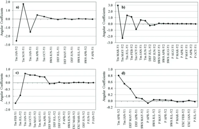
Using the sensitivity analysis, it was possible to
identify the most influential meteorological variables
for the sweet cassava yield of the São Paulo state. For this analysis, the ten best models were selected
for each region and the angular coefficients of each
independent variable were analyzed (Figure 5). The
coefficients also indicate if the influence is direct (+)
or inverse (-), in relation to the sweet cassava yield.
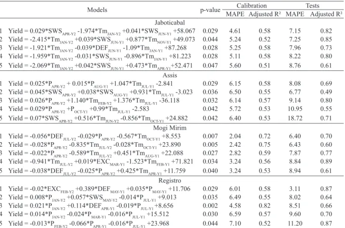
Table 1. Agrometeorological models to estimate the sweet cassava yield for the most important producing regions of the São Paulo state.
Models p-value Calibration Tests
MAPE Adjusted R² MAPE Adjusted R² Jaboticabal
1 Yield = 0.029*SWSAPR-Y2 -1.974*TmJAN-Y2 +0.041*SWSJUN-Y1 +58.067 0.029 4.61 0.58 7.15 0.82 2 Yield = -2.415*TmJAN-Y2 +0.039*SWSJUN-Y1 +0.877*TmNOV-Y1 +49.073 0.044 5.24 0.52 7.25 0.85 3 Yield = -1.921*TmJAN-Y2 -0.039*DEFJUN-Y1 -1.09*TmJAN-Y1 +87.268 0.028 5.25 0.58 7.96 0.73 4 Yield = -1.959*TmJAN-Y2 -0.031*SWSJUN-Y1 -0.896*TmJAN-Y1 +81.223 0.028 5.11 0.58 8.22 0.80 5 Yield = -2.069*TmJAN-Y2 +0.042*SWSJUN-Y1 +0.473*TmAPR-Y1+52.471 0.047 5.60 0.51 8.76 0.61
Assis
1 Yield = 0.025*PAPR-Y2 + 0.015*PAUG-Y1 +1.047*TmJUL-Y1 -2.841 0.029 6.15 0.58 8.08 0.69 2 Yield = 0.045*SWSAPR-Y2 +0.038*SWSAUG-Y1 +0.931*TmJUL-Y1 -3.023 0.036 6.50 0.55 6.77 0.49 3 Yield = 0.026*PAPR-Y2 +1.140*TmFEB-Y2 +1.376*TmJUL-Y1 -36.118 0.032 6.14 0.57 9.14 0.80 4 Yield = 0.029*PAPR-Y2 +POCT-Y1 +0.99*TmJUL-Y1 -2.583 0.042 5.72 0.53 10.95 0.55 5 Yield = 0.07*SWSAPR-Y2 +0.516*TmJUN-Y2 -0.856*TmOCT-Y1 +24.882 0.042 6.40 0.53 18.72 0.71
Mogi Mirim
1 Yield = -0.056*DEFJUL-Y2 -0.029*PAPR-Y2 -0.567*TmOCT-Y1 +8.553 0.007 2.04 0.72 6.40 0.70 2 Yield = -0.028*PAPR-Y2 -0.835*TmJUL-Y2 -0.028*TmOCT-Y1 +23.890 0.005 2.42 0.75 6.43 0.60 3 Yield = -0.022*PAPR-Y2 -0.589*TmJUL-Y2 +0.451*TmAUG-Y1 +22.088 0.027 2.82 0.59 7.87 0.77 4 Yield = -0.941*TmJUL-Y2 +0.019*EXCMAR-Y1 -1.523*TmFEB-Y1 +71.821 0.034 3.24 0.56 8.84 0.89 5 Yield = -0.038*DEFJUL-Y2 -0.025*PAPR-Y2 +0.425*TmAPR-Y1 +11.759 0.040 3.24 0.53 8.94 0.61
Registro
1 Yield = -0.02*EXCFEB-Y2 +0.389*DEFMAY-Y1 +0.035*PMAY-Y1 +11.706 0.029 6.01 0.58 3.11 0.87 2 Yield = 0.008*PJAN-Y2 +0.057*SWSMAY-Y2 -0.014*PJUL-Y1 +9.013 0.035 6.49 0.55 8.02 0.64 3 Yield = 0.021*PJAN-Y2 +0.114*DEFAPR-Y1 -0.019*PJUL-Y1 +8.656 0.002 4.58 0.82 8.51 0.66 4 Yield = 0.014*PJAN-Y2 -0.024*PMAR-Y1 -0.016*PJUL-Y1 +15.512 0.030 6.59 0.57 9.60 0.70 5 Yield = -0.013*PFEB-Y2 -0.066*PAPR-Y1 -0.016*PJUL-Y1 +23.968 0.044 7.10 0.52 11.20 0.87
MAPE: mean absolute percentage error; SWS: soil water storage (mm); Tm: mean air temperature (ºC); DEF: water deficiency (mm); P: precipitation (mm); JAN-Y1:
month of the development year (year 1); JAN-Y2: month of the production year (year 2).
The mean air temperature had a higher
frequency and higher coefficients for all regions,
mainly during the periods of physiological dormancy and harvest (January to July). Jaboticabal and Assis showed an inverse relationship, while, for Mogi Mirim and Registro, it was direct. An inverse relation indicates that an increase of air temperature
is deleterious to the final yield, and a direct relation favors the final yield.
Generally, air temperature is one of the most
important meteorological elements that affect the
cassava development (Streck 2002). At the end of the tuber bulking, and mainly at the vegetative growth (November), if temperature decreases, the formation of leaves also decreases (Schons et al. 2007). According to Fagundes et al. (2007), high temperatures during the starch accumulation phase (January) slow the leaf senescence, harming the initial starch concentration. Higher temperatures at harvest, associated with lower water supply, increase
the soil resistance, making more difficult the lifting of roots from the soil. This reduces the harvest efficiency
by increasing the lifting force and causing damage to the roots (Agbetoye et al. 1998).
With the objective of synthesizing the
information about the effects of the variables on
sweet cassava yield, an analysis of variable frequency
and coefficients was conducted with all the models
of the producing regions of the state, and showed that the mean air temperature during the whole cycle
and the water deficit and soil water storage at the beginning and end of the cycle are the most influential
meteorological variables for the production in the
Figure 5. Angular coefficient of the most influential independent variables adjusted for the ten best models to estimate the sweet cassava yield in the regions of Jaboticabal (a), Assis (b), Mogi Mirim (c) and Registro (d). Tm: mean air temperature; SWS: soil water storage; DEF: water deficiency; EXC: water excess; P: precipitation; Y1: indicates variables from the development year; Y2: indicates variables from the production year.
A: maximum anticipation; B: best model (calibration) anticipation.
Region Year 2
FEB MAR APR MAY JUN JUL
Jaboticabal A, B
Assis A B
Mogi Mirim A, B
Registro A B
São Paulo state (Figure 6). One of the reasons for the high tolerance of cassava during dry periods is its highly sensitive stomatal system. In low moisture soil conditions, the plant saves water by controlling transpiration; however, long periods with severe dry spells during the cycle decrease yield (Oliveira et al. 1982, Okogbenin et al. 2013).
Air temperatures in October and November, during phases of tuber bulking, vegetative growth and the beginning of starch accumulation were the
other variables that had a large influence on sweet
cassava yield, with a direct relation (+). At these
phases, temperatures directly affect leaf senescence,
thus favoring the root dry matter accumulation, which is higher during this period (Peressin et al. 1998).
CONCLUSIONS
1. The regional agrometeorological models were significant and showed a strong capacity to estimate the sweet cassava yield before harvest. The highest accuracy for each region was 3.11 % for Registro, 6.40 % for Mogi Mirim, 7.15 % for Jaboticabal and 8.08 % for Assis;
2. The most influent variables for the São Paulo
state, during the sweet cassava cycle, are mean
air temperature, water deficiency and soil water
storage. The mean air temperature is the most important meteorological element, mainly in periods of physiological dormancy and harvest (January to July).
REFERENCES
AGBETOYE, L. A. S.; KILGOUR, J.; DYSON, J. Performance evaluation of three pre-lift soil loosening devices for cassava root harvesting. Soil and Tillage
Research, v. 48, n. 4, p. 297-302, 1998.
ALVES, A. A. C. Fisiologia da mandioca. In: EMBRAPA MANDIOCA E FRUTICULTURA TROPICAL. Aspectos
socioeconômicos e agronômicos da mandioca. Cruz das
Almas: Embrapa, 2006. p. 138-169.
CAPORUSSO, N. B.; ROLIM, G. S. Reference
evapotranspiration models using different time scales in the
Jaboticabal region of São Paulo, Brazil. Acta Scientiarum
Agronomy, v. 37, n. 1, p. 1-9, 2015.
COMPANHIA NACIONAL DE ABASTECIMENTO (Conab). Levantamentosafra 2015-2016. 2017. Available
at: <http://www.conab.gov.br>. Access on: 16 Feb. 2018.
CORREA, S. T. R. et al. Aplicações e limitações da modelagem em agricultura: revisão. Revista de
Agricultura, v. 86, n. 1, p. 1-13, 2011.
DOORENBOS, J.; KASSAM, A. H. Efeito da água no
rendimento das culturas. Campina Grande: UFPB, 1994.
FAGUNDES, L. K. et al. A fenologia da mandioca em diferentes épocas de cultivo em local de clima subtropical.
Raízes e Amidos Tropicais, v. 3, n. 1, p. 1-4, 2007.
FOOD AND AGRICULTURE ORGANIZATION OF THE UNITED NATIONS (FAO). Faostat database
collections. Rome: FAO, 2012.
FOOD AND AGRICULTURE ORGANIZATION OF THE UNITED NATIONS (FAO). Save and growcassava:
a guide to sustainable production intensification. Rome:
FAO, 2013.
GABRIEL, L. F. et al. Mudança climática e seus efeitos na cultura da mandioca. Revista Brasileira de Engenharia
Agrícola e Ambiental, v. 18, n. 1, p. 90-98, 2014.
GUJARATI, D. N.; POTER, D. C. Econometria básica. 5. ed. Porto Alegre: AMGH, 2011.
INSTITUTO BRASILEIRO DE GEOGRAFIA E ESTATÍSTICA (IBGE). Levantamento sistemático da
produção agrícola. 2016. Available at: <https://www.ibge.
gov.br/estatisticas-novoportal/economicas/agricultura-e-pecuaria.html>. Access on: 26 Feb. 2018.
LAHAI, M. T.; GEORGE, J. B.; EKANAYAKE, I. J. Cassava (Manihot esculenta Crantz) growth indices, root yield and its components in upland and inland valley ecologies of Sierra Leone. Journal of Agronomy and Crop
Science, v. 182, n. 4, p. 239-248, 1999.
MEZZETTE, T. F. et al. Selection of sweet cassava elite-clones for agronomical, technological and chemical characteristics. Bragantia, v. 68, n. 3, p. 601-609, 2009.
MORETO, V. B.; ROLIM, G. S. Estimation of annual yield and quality of ‘Valência’ orange related to monthly water
deficiency. African Journal of Agricultural Research, v. 10, n. 6, p. 543-553, 2015.
OKOGBENIN, E. et al. Phenotypic approaches to drought in cassava: a review. Frontiers in Physiology, v. 4, n. 93, p. 1-15, 2013.
OLIVEIRA, S. L.; MACEDO, M. M. C.; PORTO, M.
C. M. Efeito do déficit de água na produção de raízes de
mandioca. Pesquisa Agropecuária Brasileira, v. 17, n. 1, p. 121-124, 1982.
PERESSIN, V. A. et al. Effects of weed interference on
cassava growth and productivity. Bragantia, v. 57, n. 1, p. 135-148, 1998.
RIJKS, D.; BARADAS, M. W. The clients for agrometeorological information. Agricultural and Forest
Meteorology, v. 103, n. 1, p. 27-42, 2000.
RÓS, A. B. et al. Cassava cultivars growth, phenology and yield. Pesquisa Agropecuária Tropical, v. 41, n. 4, p. 552-558, 2011.
SÃO PAULO. Coordenadoria de Assistência Técnica Integral (CATI-LUPA). Levantamento censitário das unidades de produção agropecuária do estado de São
Paulo. 2008. Avaible at: <http://www.cati.sp.gov.br/
projetolupa/mapaculturas/Mandioca.php>. Access on:
13 Feb. 2018.
SCHONS, A. et al. Emissão de folhas e início de acumulação de amido em raízes de uma variedade de mandioca em função da época de plantio. Ciência Rural, v. 37, n. 6, p. 1586-1592, 2007.
STRECK, N. A. A generalized nonlinear air temperature response function for node appearance rate in muskmelon
(Cucumis melo L.). Revista Brasileira de Agrometeorologia,
v. 10, n. 1, p. 105-111, 2002.
THORNTHWAITE, C. W. An approach towards a rational
classification of climate. Geographical Review, v. 38, n. 1, p. 55-94, 1948.
THORNTHWAITE, C. W.; MATHER, J. R. The water
balances. Centerton: Drexel Institute of Technology, 1955.
TREMACOLDI, C. R. Manejo das principais doenças da cultura da mandioca no estado do Pará. In: MODESTO JUNIOR, M. S.; ALVES, R. N. B. (Eds.). Cultura da
mandioca: aspectos socioeconômicos, melhoramento
genético, sistemas de cultivo, manejo de pragas e doenças e agroindústria. Brasília, DF: Embrapa, 2016. p. 162-170.
VALLE, T. L. et al. Cyanide and acid content in progenies from crosses of bitter and sweet cassava cultivars.
Bragantia, v. 63, n. 2, p. 221-226, 2004.
VALLE, T. L. et al. Mandioca: energia e alimento para o mundo. O Agronômico, v. 59, n. 1, p. 29-31, 2007. VALLE, T. L.; LORENZI, J. O. Improved varieties of cassava as a tool of innovation, food safety, competitiveness and sustainability: contributions of the Agronomic Institute of Campinas (IAC). Cadernos de Ciência e Tecnologia, v. 31, n. 1, p. 15-34, 2014.
WALPOLE, R. E.; MYERS, R. H.; MYERS, S. L.
Probability & statistics for engineers & scientists. 9. ed.
Boston: Pearson Education, 2012.
ZANETTI, E. G. B. et al. Performance of two cassava
varieties submitted to different spacings, grown in the
Cerrado region. Brazilian Journal of Applied Technology