Analysis and Improvement of a Rubber Agglomeration Manufacturing Process using a Discrete Event Simulation Model

Analysis and Improvement of a Rubber Agglomeration Manufacturing

Process using a Discrete Event Simulation Model

Ricardo Campos Maia

Dissertação de Mestrado

Orientador na FEUP: Prof. Mário Amorim Lopes Orientador na empresa: Mike Bain

Mestrado Integrado em Engenharia Mecânica

Resumo

Um aumento da concorrência global, aliado a níveis de consumo cada vez mais altos, aumen-tou a necessidade das empresas em produzir produtos em maiores quantidades, com melhor qualidade e em espaços de tempo mais curtos. Desta forma, é necessária a adoção de estraté-gias que permitam obter níveis mais altos de eficiência.

O projeto foi realizado numa linha de produção de cilindros de borracha, cujo objetivo princi-pal se baseou na análise e melhoria do processo produtivo recorrendo a uma ferramenta de simulação. Estando a ferramenta criada, foi possível estudar a reengenharia do processo expe-rimentando várias estratégias produtivas. A simulação é vantajosa na medida que possibilita o teste de diferentes cenários sem afetar a produção, e consequentemente sem custos associa-dos.

A principal adversidade está relacionada com os diferentes valores das taxas de entrada e saí-da de matéria-prima nos silos. Uma taxa de saísaí-da mais elevasaí-da cria um défice produtivo que esgota o material disponível nos silos, forçando uma mudança de produção. Esta situação atrasa a produção uma vez que se produzirão artigos não urgentes, para stock, até os silos se-rem reabastecidos.

Recorrendo ao modelo desenvolvido foi possível identificar ineficiências no processo de car-regamento dos silos que restringia o fluxo de entrada e reduzia os ciclos produtivos. Ao eli-minar tais ineficiências, concluiu-se que a produção poderia ser estendida pelo tempo deseja-do. Assumindo tal situação, pode-se descartar o cenário que contemplava a adição de um no-vo silo. Por outro lado, concluiu-se que ao implementar tal melhoria seria possível estender a produção a dois turnos diários, sem falhas de matéria-prima.

Ao analisar o processo produtivo foi também identificado o gargalo do mesmo. Procedeu-se à simulação de dois cenários distintos, representativos de aumentos de velocidades de produção diferentes, de forma a avaliar o impacto que teriam na disponibilidade da matéria-prima. Con-cluiu-se que apenas era vantajoso aumentar a velocidade de produção se fosse mantido um turno diário, aliado a um aumento da taxa de entrada de material nos silos.

Recorrendo ao OEE pode-se analisar as perdas ocultas de produtividade. Os resultados obti-dos mostram que a baixa disponibilidade do equipamento proporcionava a maior oportunida-de oportunida-de melhoria. As principais razões estão relacionadas com os tempos oportunida-de transição entre sé-ries e paragens não planeadas. Na linha procedeu-se à implementação de vários aperfeiçoa-mentos, de forma a proporcionar um ambiente mais organizado e limpo aos operadores. Os objetivos do projeto foram alcançados e é expectável que os resultados obtidos possam permitir à empresa perspetivar as consequências que advêm da implementação de várias estra-tégias produtivas.

Abstract

An increasingly fierce global competition and high product demand has forced companies to produce more goods, with a better quality in less time. To achieve this, new strategies that grant higher efficiency levels, had to be enforced.

This project took place in a rubber agglomeration manufacturing line. The main goal was to analyse and improve the productive process recurring to a simulation tool. Once the tool was created it was possible to reengineer the process by experimenting with different scenarios. It has the advantage of testing different alternatives without disrupting the production line and consequently with no associated costs.

The main issue was related with the difference of material rates, in and out of the silos. A higher out-rate creates a material deficit that drains the silos after a few days, forcing produc-tion to be adjusted. This delays producproduc-tion as it will be manufacturing non urgent stock arti-cles until the silos levels are replenished.

With the model it was possible to identify inefficiencies in the material loading operations that hindered the in-rates and shortened the production lifecycle. By addressing this issue, production is expected to be able to resume for the expected duration. Therefore, the testing scenario that simulated the impact of adding an extra silo was discarded. On the other hand, a double daily shift could be enforced without expected material shortages.

Afterwards, the production process was examined and the “Bottleneck” operation was identi-fied. Two distinct scenarios, representing different production speed increases, were tested to evaluate their impact on raw material availability. It was concluded that only by maintaining a single shift and enhancing loading operations could the speed increase benefit the process. The OEE tool was applied to unveil hidden productivity losses. It was disclosed that the main issue relied on the low availability rates. The main reasons were related to changeovers and unplanned stops. On the production line, some improvements were made in order to provide operators with a safer, cleaner and more organized working space.

The project’s objectives were accomplished and it is expected that the obtained results could offer the company an insightful perspective on the consequences of implementing different productive strategies.

Acknowledgments

Firstly, I would like to thank Amorim Cork Composites for providing me with a fulfilling and dynamic working experience overseas, where I had exceptional conditions to develop my project.

I would like to extend my gratitude to all the members of ACC USA that made it easy for me to adapt to a new reality, in such a welcoming and supporting manner. I would like to give a special thanks to Mike Bain for its availability and constant support throughout the duration of the project.

To my professor, Mário Lopes, I would like to thank for guiding me towards simulation mod-elling, that I found out to be such an interesting and useful skill to learn. Thank you for men-toring me throughout the entire process and for always being available in such short notices. I would also like to acknowledge Nanci Carvalho, for the constant monitoring which made me feel supported during the entire experience.

Last of all, I would like to thank my close family for always supporting me in every aspect of my life and encourage me to constantly step out of my comfort zone to pursue my goals. Thank you for all the opportunities given throughout my life, which defined my journey and myself as a person.

INDEX

1 Introduction ... 1

1.1 Aim of the thesis ... 1

1.2 Amorim Cork Composites – a brief introduction ... 1

1.3 Project Objectives ... 3

1.4 Methodology ... 3

1.5 Dissertation structure ... 4

2 Literature review ... 5

2.1 Production and Operations management ... 5

2.2 Analytical methods applied to Production and Operations Management ... 5

2.2.1 Process Mapping ... 6

2.2.2 Value Stream Mapping ... 6

2.2.3 Simulation modeling... 8

2.2.4 Bottleneck analysis and theory of constrains ... 13

2.3 OEE indicator ... 13

3 Case study ... 15

3.1 Production policy and demand levels ... 15

3.2 Production line overview ... 15

3.2.1 Productive process ... 16

3.2.2 Production area constraints ... 18

3.2.3 Key parameters that influence production planning ... 19

3.3 Black buffing amounts deficit ... 20

4 Simulation modelling ... 22

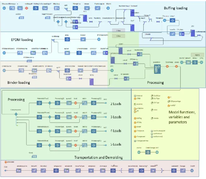
4.1 Model overview ... 22

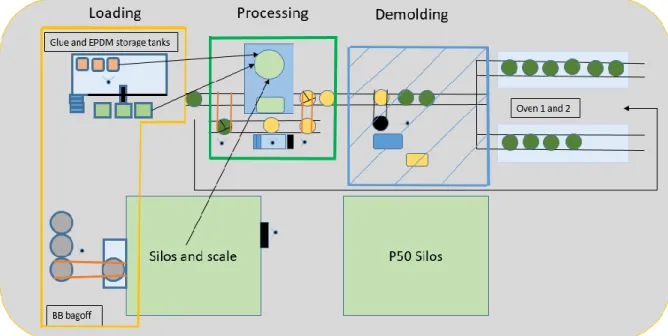
4.2 2D Interface ... 22

4.3 Main interface ... 24

4.3.1 Logical blocks libraries ... 24

4.3.2 Simulation process analysis ... 25

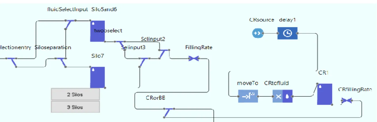
4.3.3 Sub-processes ... 26

4.4 Model validation ... 31

4.5 Error discrepancy causes ... 33

5 Production improvement ... 34

5.1 Buffing consumption ... 34

5.2 Loading scenarios ... 35

5.3 Black buffing exclusive production sets ... 37

5.4 Production hypothesis ... 38

5.4.1 Testing Assumptions... 38

5.4.2 Third silo addition ... 39

5.4.3 Double shift ... 40

5.4.4 Bottleneck identification ... 42

5.4.5 Production Speed Increases ... 42

5.4.5.1 Ideal scenario ... 46

5.5 Achieving the “Improved” Scenario ... 47

5.6 OEE analysis ... 48

Conclusions ... 50

References ... 52

Appendix A: Model’s Entities ... 57

Appendix C: Model validation analysis with an outlier ... 59 Appendix D: Production line improvement suggestions ... 60 Appendix E: 3 Loading Scenario Analysis ... 63

Abbreviations

ABM - Agent Based Model ACC - Amorim Cork Composites APE - Absolute Percentage Error BB - Big Bag

EBM - Event Based Model

MAPE - Medium Absolute Percentage Error MTS - Make To Stock

MTO - Make To Order

OEE - Overall Equipment Effectiveness TOC - Theory Of Constraints

TPM - Total Productive Maintenance WIP - Work In Progress

List of Figures

Figure 1 - “Mold Room” location... 2

Figure 2 - Simulation model creation methodology by Rabe, Spieckermann, & Wenzel ... 4

Figure 3 - Simulation approaches comparison (Borshchev, A. (2013)) ... 9

Figure 4 - Comparison between ABM and EBM features (Baldwin, Sauser and Cloutier, 2015). ... 9

Figure 5 - OEE time losses overview ... 14

Figure 6 - 2016 Production share by reference... 16

Figure 7 - Raw materials: buffing stored in BB's, EPDM and binder ... 16

Figure 8 - Bagoff equipment and EPDM tanks ... 17

Figure 9 - Silos and mixing process ... 18

Figure 10 - Oven loading and demolding operations ... 18

Figure 11 - Sector division by areas ... 19

Figure 12 - The 4 stages of the bag loading operations ... 20

Figure 13 - Loading operations duration breakdown ... 21

Figure 14 - 2D productive process representation ... 23

Figure 15 –Most relevant Anylogic blocks used from both libraries ... 24

Figure 16 - Main ... 25

Figure 17 - Buffing loading block scheme, phase 1 ... 26

Figure 18 - Buffing loading block scheme, phase 2 ... 27

Figure 19 - EPDM loading block scheme ... 27

Figure 20 - Binder loading block scheme ... 28

Figure 21 - Processing operations block scheme ... 28

Figure 22 - Transportation and demolding operations block scheme ... 29

Figure 23 - Part of the model's control elements ... 30

Figure 24 - Production planning template ... 30

Figure 25 - Simulation model data inputs ... 31

Figure 26 - APE obtained during 49 production days ... 32

Figure 27 - Available amount of black buffing during a three day production sequence ... 35

Figure 28 - Comparison of the different black buffing amounts available in each one of the 3 scenarios ... 36

Figure 29 - Comparison of a production run simulating the impact of CR products ... 37

Figure 30 - Amount of buffing in the silos – Extreme set ... 39

Figure 31 - Amount of buffing in the silos – Mild set ... 40

Figure 33 - Buffing amount on the silos - single shift - "Improved" – “Extreme” and “Mild”

sets ... 44

Figure 34 - Buffing amount in the silos - double shift - "Improved" – “Extreme” and “Mild” sets ... 45

Figure 35 - Buffing amount in the silos - single shift - "Ideal" – “Extreme” and “Mild” sets . 46 Figure 36 - OEE analysis results ... 49

Figure 37 - Availability losses causes (A) and Unplanned Stops causes (B) ... 49

Figure 38 - Entities usage sequence ... 57

Figure 39 - Black rubber buffing ... 58

Figure 40 - 50 day APE analysis, with an outlier ... 59

Figure 41 - “Before” and “After” pictures of the production’s line storage area ... 60

Figure 42 - Efficiently organized tools ... 61

Figure 43 - Spare parts properly organized ... 61

Figure 44 - Loading operations improvement measure ... 62

List of Tables

Table 1 - Comparison between the different available software (Mourtzis, Doukas &

Bernidaki, 2014) ... 11

Table 2 - Part of the spreadsheet used to compare simulation runs with the daily production 31 Table 3 -Model validation data ... 33

Table 4 - Production related data ... 34

Table 5 - Comparison between the three different operations loading scenarios ... 36

Table 6 - Operation’s duration breakdown ... 38

Table 7 - General overview of the extra silo adding situation... 40

Table 8 - Productive process operations ... 42

Table 9 - Production speed increases comparison ... 43

Table 10 - Resource’s Availability- Mold and Buffing ... 43

Table 11 - Production length comparison between various tested scenarios on “Improved" scenario ... 45

Table 12 - Production length comparison between various tested scenarios on an “Ideal" scenario ... 46

1 Introduction

The production of rubber cylinders is a highly complex process, involving heavy industrial equipment that is part of a stationary manufacturing structure with an inflexible layout. Changes to the production process may require shutting down the line for days, if not weeks, which would incur in huge costs, and eventually a failure to fulfill production orders in time. However, such scenario should not lead to inaction, in this way avoiding improvements alto-gether that could contribute to a more efficient production process, saving scarce resources or increasing production throughput. Hence, addressing this problem without disrupting the pro-duction with experimentation requires a method capable of simulating and inspecting the rub-ber production process, while at the same time providing the tools to experiment with changes and measure their potential impact on key indicators.

In this dissertation we devise a simulation-based method to reproduce the rubber cylinder manufacturing line, and illustrate its application on a real case study. We validate the model by comparing virtual and real production times, and once deemed to be accurate we experi-ment with several potential improveexperi-ments, measuring their impact. We believe this methodol-ogy may be a sound contribution to the rubber production industry, helping to improve the production process in a controlled and prudent manner.

1.1 Aim of the thesis

The present project was developed at the Amorim Cork Composites (ACC) manufacturing plant, in Wisconsin, USA. ACC is a Portuguese company, part of the Corticeira Amorim’s group. Although the company’s main business is cork, this plant is directed towards the man-ufacturing and processing of rubber agglomerates products. The respective production line will be the project’s central focus.

Its primarily objective is to scrutinize the productive system and seek improvement opportuni-ties, while eliminating inefficiencies, as well as projecting the consequences derived from im-plementing different production strategies.

1.2 Amorim Cork Composites – a brief introduction Amorim Group

Amorim Group is a Portuguese multinational company that had its roots in the cork business back in the 1870’s under the name of “Corticeira Amorim”. Although still being its core busi-ness, the group aimed at a business diversification process in the early 1960’s. Now the Amo-rim Group has well established positions in sectors as distinct as the financial, textile, com-munications, tourism and real estate, being one of the most dynamic and well succeeded groups in Portugal.

Corticeira Amorim

The company is the worldwide leader in the cork sector. Guided by a vision of sustained growth and quality excellence in their products, the company grew internationally to a global scale. The mission is to: “Add value to cork in a competitive, distinctive and innovative way

that is in perfect harmony with nature”. It currently holds 83 companies, 29 industrial plants,

44 distribution companies, 11 joint ventures and 258 main agents spread throughout the world.

Amorim Cork Composites

Amorim Cork Composites (ACC) is a subgroup of Corticeira Amorim that resulted from the merge of 2 of the group’s now defunct companies (Amorim Industrial Solutions and Amorim Indústria). Its main business is composite cork and arose from the need of reusing the waste that came from the bottle cork industry. It is also responsible for constantly seeking new ap-plications for cork that can be used in an increasingly higher number of products. Their mis-sion is: “Reinventing how cork engages the world”.

In 2007 an overseas facility in Trevor, USA (former Amorim Industrial Solutions) was added to ACC. This plant’s main business is rubber agglomeration manufacturing, which transforms reground rubber granulates into finished goods that may include: flooring material, underlays, rubber blocks and logs, among others. Although there is no cork production in Trevor, the plant often imports sizable amounts of this material from Portugal, enabling it to hold a share of the American cork market.

ACC USA – Agglomeration Sector

The plant is divided in three main areas: Agglomeration, Transformation and Storage and Shipping operations.

The project was developed in the main production area of the plant: the rubber agglomeration manufacturing line, also designated as the “Mold Room” and represented by Figure 1. In this place, a transformation process turns rubber buffing into rubber blocks or cylinders (Logs). After being produced these materials follow through to the remaining sectors, so they can be transformed into finished items, stored and shipped.

Figure 1 - “Mold Room” location

All of the plant’s productivity depends on the efficiency of this manufacturing process as it is the first step of the interdependent internal productive chain. Without it, all the subsequent sectors would starve. Therefore it is on the company’s best interest to reduce inefficiencies and extend production time within this sector, thus improving efficiency and productivity. This will have a positive effect which will be reflected on the entire plant’s performance.

Operations are run 6 days per week and three different product types are manufactured during that period. A problematic situation arises during the Log production days, which occupy production during 3-4 days a week. When producing Logs, the silos, which store black buff-ing, are drained at faster rates than they are refilled, creating a deficit. This deficit will even-tually cause the silos to be emptied, forcing production to be temporarily switched to low-priority colored buffing products, while they are being refiled. This causes urgent orders to be delayed and the production schedule to be hampered.

1.3 Project Objectives

The proposed project main field of action would concern the Rubber Agglomeration manufac-turing line process, during the production of Rubber Logs. With the objective of improving the process in its whole, several objectives were set:

1. The first, and most relevant goal, was to develop a simulation model that could reproduce the productive system with accuracy. This would allow for a complete process analysis without any associated costs and without disrupting the actual productive system. After being created and validated, this tool would be used to test the following scenarios and its respective impact on the black buffing material availability:

1.1. Extended production cycles, with more efficient loading operations; 1.2. Use of an extra storage material;

1.3. Double daily shift implementation; 1.4. Production speed increase;

2. Identify the causes and extent of hidden productivity losses using an OEE analysis; 3. Apply LEAN methods to the sector:

3.1. Improve work conditions on the line by using the 5S methodology;

3.2. Suggest Standard work to eliminate inefficiencies on the line and prove that a better performance levels can be achieved.

1.4 Methodology

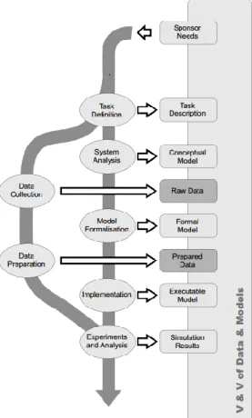
The simulation project was divided in five main stages: Identifying the company’s require-ments, developing a strategy to represent the productive system in a simulation tool, gathering the necessary data to do it and creating the respective model, executing and validating it, and lastly experimenting various alternatives and analyzing the respective results. This was based on a methodology by (Rabe, Spieckermann, & Wenzel (2009), represented by Figure 2. At the same time a 5S methodology was followed to improve working conditions within the produc-tion line.

 Phase 1 – The first phase involved the full understanding of the complete productive pro-cess, as well as the company’s needs for the sector;

 Phase 2 – Defining the plan of action. This phase involved depicting the most relevant processual phases that should be portrayed in the model;

 Phase 3 - After having a strong understanding of the process and having a plan defined, all the relevant data started being gathered, which would be later applied to the model. Concurrently, a conceptual model started being developed. Meanwhile, several line im-provements opportunities were identified;

 Phase 4 - After having the model created, the prepared gathered data was added, generat-ing a functional tool that was later validated recurrgenerat-ing to production sheets;

 Phase 5 – By having an executable, validated model new production strategies could be simulated and their results analyzed. Production line improvements were also implement-ed in this phase.

Figure 2 - Simulation model creation methodology by Rabe, Spieckermann, & Wenzel

1.5 Dissertation structure

This project is divided in 6 chapters. The following two chapters present the initiation phase that preceded the development of the simulation model. On Chapter 2, a literature review re-garding the state of the art of the most relevant themes is addressed, while Chapter 3 exposes the production’s line current situation. Chapter 4 presents and explores the developed simula-tion model, followed by Chapter 5, which exposes several testing experiments made and their respective outcomes. On Chapter 6 the project’s conclusions are presented and possible future works are suggested.

2 Literature review

2.1 Production and Operations management

Operations management is the group of managerial systems and processes responsible for the production of goods and services. It differs from other management areas due to the involve-ment of both people and equipinvolve-ment (Stevenson, 2009). Therefore, there is a need to create strategies that englobe both of these elements within the organization. Lately, there has been a wider number of researches that, in addition to focusing just on the equipment elements of the productive chain, also start considering the impact of the human element (Westbrook, 1995). Production, or manufacturing, involves the transformation of raw material (input) into a fin-ished good (output). This transformation process involves several phases and distinct re-sources. There is also a need to assure quality standards, therefore production control is man-datory throughout the entire process.

By going through this transformation process, value is being added to the product, which will be reflected on the amount customers will be willing to pay for it. Expectedly, this value will be higher than the sum of all the input related costs, resulting in profit for the organization (Stevenson, 2009).

During the course of the years, the manufacturing industry as evolved in order to cope with the increasingly demanding challenges of the modern world. Consequently, new and more efficient production methodologies were created and adopted.

2.2 Analytical methods applied to Production and Operations Management

In order to properly assess a productive process, it is necessary to use a method capable of producing an acceptable outcome. This method should be able to reproduce the productive process accurately, as well as being able to reengineer it if needed. The most widely used methods are the following:

- Process Mapping. It is based on a workflow diagram with the main purpose of providing a clear understanding of the productive process. It relies mainly on the use of flowcharts. The main difference between industrial and digital process mapping re-sides on the fact that it identifies the participants alongside the processes. It is divided in three major phases that involve the creation of three respective models: “As-Is”, “To-Be” and “Bridging the Chasm” (Okrent & Vokurka, 2004);

- Value Stream Mapping. It is the analysis of a group of actions (value added and non-value added actions) required to move a product through the complete production flow: from raw material to finished product. It displays the process’s “big picture”, al-lowing focus to be drawn on improving the process as a whole, instead of targeting smaller individual parts (Rother & Shook, 2003);

- Simulation Modelling. It accurately represents a production process. It will allow for the testing of several alternatives without associated costs and without disrupting the production line. It is useful to test the impact that a preplanned measure will have on the system, as well as improving it by detecting and eliminating inefficiencies (Pedgen, Shadowski, & Shannon, 1995);

- Bottleneck analysis and theory of constraints. The system’s bottleneck is the most time consuming operation, which hinders production rates and will cause material ac-cumulation before its respective station. The theory of constrains is a sequenced meth-od designed to analyze and improve the system’s constraints, improving performance and efficiency (Lanke, Hoseinie & Ghodrati, 2016).

2.2.1 Process Mapping

The main objective of Process Mapping is to use diagramming tools, such as flowcharts, in order to display all the possible processual outcomes of every operation, enabling an organi-zation to improve its efficiency. By having processes identified, as well as inputs, outputs and decision points, it is possible to attain a clearer global perspective and assess if and how im-provements can be promoted inside the organization. According to Okrent & Vokurka in 2004, process mapping can be divided in 3 phases.

Phase 1- “As-Is” Model. It is vital to understand how processes are currently performed and

the main reasons for it. All the interconnections between processes should be sequenced ac-cording to their execution order. This will allow for the detection of non-value added activi-ties that can be reduced or removed, when transitioning to the “To-Be” model.

Phase 2 –To-Be” Model. Firstly, while creating this model the main focus should be on

iden-tifying the critical, strategical, business processes. Next, a flowchart with no constraints should be elaborated. Then, taking into account all of the system’s restrictions, a simplifica-tion process should take place to reduce and simplify the process before automating it.

Phase 3 - “Bridging the Chasm” Model. It is the intermediate model that will allow for a

smooth transition between the two previous phases, without major productivity losses.

This reengineering method has proven to produce adequate results for every company in need of more efficient processes. By identifying the current process flows it is possible to locate inefficiencies and aim for the desired objectives, following a structured transition. Although it can be used in both information and material flow projects, it has predominant applications on the information flow field.

2.2.2 Value Stream Mapping

It surfaced alongside the Lean methodology in order to redesign the productive systems in a more efficient manner. What differentiates VSM from other processes is that it focuses on representing the two main flows involved in any industry: information and material flow. Its main goal is to grant visibility to the entire process, so it can be studied and improved as a whole, detecting inefficiencies and disconnected manufacturing flow lines.

In order to do so, it has to consider all the activities required to manufacture a product. These can be divided in: value added activities and non-value added activities. The first group gath-ers all the operations in which the final result diffgath-ers from the initial result, in both shape and value. These include all the processing operations required to transform raw materials in mar-ketable items, for which clients are willing to pay for (Singh, Garg & Sharma, 2011).

The second group is considered to be included in one of the Lean methodology’s three main wastes: Muda. It states that any activity that does not add value to the product is a waste of resources and should be reduced or eliminated. It is often related to excessive transport

movements, of parts and resources, prolonged waiting times and inaccurate production plan-ning. This will cause inventory surplus and overproduction, reducing the production flow and increasing Work in Progress (WIP). Although some of the non-value adding activities are necessary to establish a production system, others can be significantly reduced (Pinto, 2008). According to Rother and Shook in 2003, every VSM project is based in five different phases:

- Selection of the product family. It is vital to extend the analysis to all the variants within the same product family, which share flow routes throughout the manufacturing process;

- Current state analysis. Evaluate the current situation by integrating all the relevant parameters and processes in a map that reproduces the entire system. All the flow stages must be represented, as well as the duration it takes for each operation to be completed. In order for VSM to produce accurate results there must be a rigorous data gathering procedure. These will have a major effect on the conclusions drawn from the method. Poorly collected data will consequently result in a poor decision making pro-cess. As the process’s inefficiencies are revealed by the collected data a strategic plan for improvement should be commenced;

- Future state analysis. The future state analysis includes a redesign of the productive process that should embody several Lean principles. Firstly, there should be a lower reliance on forecasts as production rates should directly represent real product demand based on orders. This production adjustment is represented by takt times. Implement-ing a pull system is also a critical step in the process. Material must not accumulate in-between operations, creating Muda by increasing WIP. It should only advance if the following station is vacant. Cycle time decreases and changeover reductions imple-mentation could further benefit the productive system;

- Designing a plan of action. A plan must be drawn to expose how the Future state sit-uation will be achieved. A chronogram including every relevant transformation time frame should also be contemplated;

- Implementing the plan. The last phase includes the execution of the previously de-lineated plan and the result’s evaluation.

Application of VSM in the industry

In terms of application, VSM has been widely used in several industries over the last two dec-ades. The revamping of a distribution network for electronic components was reviewed by Brunt, Sullivan, Hines in 1998, which involved a prior analysis of the current stream flow and was proceeded by the implementation of an improvement plan that englobed dozens of sup-pliers. Taylor (2005) studied how a value stream analysis allowed the discovery of hindering system inefficiencies in a complete food supply chain, which involved all the processes from the farmer to the final client. Another project, using VSM in the food and drinking sector, de-tected significant improvement opportunities while reducing and eliminating non value added activities (Melvin, Baglee, 2008). Also, by using the VSM a forging industry was able to sur-pass their inability to reduce wasteful operations by identifying their causes and eliminate them. Reductions on both set up and WIP levels were also attained (Sahoo, Singh, Shankar & Tiwari, 2008).

VSM and Simulation modelling

Both of these methods are often used together in order to produce a more robust analysis of a company’s situation, complementing one another. After addressing the VSM current state sit-uation and identifying the critical points in terms of improvements opportunities, a simulation model was created to test and analyze the outcomes of such measures without disrupting the production line of a Taiwanese plant (Huang & Liu 2005). In the process sector, a simulation

model was developed to provide an insightful perspective of the benefits of implementing

Lean measures with a before and after scenarios display. These opportunities were identified

via VSM (Abdulmalek & Rajgopal 2007). In a construction industry there was a need to in-crease material flow, which was achieved by studying various production scenarios on a simulation model. It was concluded that the system would become increasingly leaner if ma-terial spent lesser time on the value stream (Al-Sudairi 2007). A discrete event simulation modeling applied to a VSM process was able to increase the efficiency levels of a warehouse distribution center by identifying and eliminating faulty operations. These methods can be used separately or combined to identify and improve ineffective situations. Both are powerful tools that provide high value by granting an insightful viewpoint to the production’s current issues and the respective impact of alternative solutions.

2.2.3 Simulation modeling

Simulation modeling reproduces a real world process over time, which is displayed in a digi-tal format. It allows data gathering and an insightful representation of every stage of the pro-cess modeled, culminating in the observation of key behaviors (Pedgen, Shadowski, & Shan-non, 1995; Schelling, 1978). Being a valid imitation of the process it has the advantage of ex-perimenting, creating and optimizing every possible situation. Scenarios can be tested, with-out any disturbance or risk to the actual system (Pedgen, Shadowski, & Shannon, 1995). The model assumes an abstraction level, which may vary in each case, and has to be defined stra-tegically beforehand. However, every model will always be less complex than their real world counterpart (Borshchev, 2013).

The models can be divided regarding their dependence on time, by being static (independent) or dynamic (dependent). A dependent model can still be classified as discrete or continuous, depending on how the time scale is considered. By further scrutinizing a discrete model, a dif-ferentiation can be made, depending if a system alteration was time or event-triggered, by having event-driven or time-stepped simulations (Mourtzis, Doukas, & Bernidaki, 2014).

Events

An event is an occurrence that takes place in a specific time frame, although it does not have any duration (Bækgaard, 2004). It is vital to understand the causes, consequences, relation between events and types of events to fully comprehend the process (Granat, 2006). “Equip-ment starts moving” and “Button is pressed” can be seen as phenomenon examples. Phenom-enon are categorized as events when it is assumed that any further division has no real value, therefore their duration is suppressed. Events can be seen and may trigger activities. On the other end, activities are event-triggered and event-interrupted (Bækgaard, 2004).

Modeling types

Every model must be created to serve a well-defined purpose, with a clear objective, while being based on an existing system. This will influence the choice of method, regarding the abstraction level required. There are three main methods, and whilst “System Dynamics” is recommended for strategic, high abstraction modelling, Agent-Based and Discrete event modelling focus on more detailed, tactical or operational scenarios, at the meso or micro lev-els (Borshchev, 2013). Figure 3 illustrates the main differences between the approaches.

Figure 3 - Simulation approaches comparison (Borshchev, A. (2013))

Agent-Based Modelling

We can separate these last two approaches by the way a system is looked at. If there is a deeper understanding of the object’s behavioral qualities, when compared to the general sys-tem dynamics, a bottom-up perspective should be considered. An Agent based model (ABM) would be the most appropriate (Baldwin, Sauser, & Cloutier, 2015). These objects are referred as agents and have their own behaviors, which can be pre-defined by a set of rules.

Usually, agents also have a notion of state and will act accordingly (Borshchev, 2013). “An agent is a distinct software program that represents social actors which may be people, ani-mals, organizations or any individual system” (Baldwin, Sauser, & Cloutier, 2015). By con-necting this autonomous agents it is possible to study their interactions with each other and with the environment they are in, which can have its own dynamics as well. A spreading epi-demic model would be a suitable example for an agent based model (Borshchev, 2013).

Event-Based Modelling

The event-based models (EBM) represent a sequence of events that are performed across enti-ties, having an instantaneous impact on the process and a change in its state (Borshchev, 2013). Rather than being action programmed like the ABM, the EBM are reaction pro-grammed, passive, so it is vital for the modeler to correctly map the states and events of the system (Baldwin, Sauser, & Cloutier, 2015). Any action will be determined by the process flowchart, which will not allow any independent behaviour (Borshchev, 2013). When creating the model, there is simplicity associated with EBM, not only on the process modelling itself, but also because there is no interest in the internal states of the system, only in observable events that trigger the reactions. This allows for an easier, more convenient, method to vali-date the testing model. A manufacturing industry, where there is a transformation of raw ma-terials into finished products throughout several phases, it is a suitable EBM example (Bald-win, Sauser, & Cloutier, 2015). A comparison between these two types of models is displayed in Figure 4.

Discrete Event Simulation

The discrete event simulation (DES) is also known for solving complicated issues that other-wise would not be possible just owing to analytical human abilities. In complex process in-dustries it would not be possible to monitor the effect that every minor change would have on the system, without computer assistance. It allows for a transparent view over every stage of the process, therefore allowing for a clear bottleneck identification. It also comes as a valua-ble tool in terms of decision making processes (Donhauser, Rackow, Hirschbrunn, Schuder-erb, & Franke, 2016). Different situations regarding investment, resources allocation and op-timization policies using DES are an increasingly common practice in the industry (Gomes, & Trabasso, 2016).

Another advantage of the DES arises in plants where the layout is inflexible and Lean princi-ples and Toyota Production System measures cannot be applied to their full potential. A rigid sub process machine disposal and a heavy goods transportation system would benefit most from organizational measures rather than optimization measures (Donhauser, Rackow, Hirschbrunn, Schudererb, & Franke, 2016).

Alternative Simulation Approaches

Multimethod approaches can also be an interesting choice regarding complex industries with large scale manufacturing systems. According to Sadeghi, Dauzère-Pérès, and Yugma (2016), who conducted a study on the semiconductor industry, if there is a need for flexibility (ABM), as well as the need of queues and discrete events processing (EBM), a combination of the two methods can be applied. A process can be modelled inside the agents, through discrete events, or having the agents become entities that go through different stages while using the system. This allows to overcome the shortcomings presented in the EBM for large scale systems, re-garding modelling time and costs (Sadeghi, Dauzère-Pérès, & Yugma, 2016).

There is another option for industries that deal with bulk or high speed flows (e.g. mining, oil and packaging industry), where EBM is not fully adjusted or too slow. It is called Discrete Rate Simulation and it is a continuous modelling approach which can support discrete events as well (Siprelle, & Phelps, 1997). The main drawback is the loss of information inherent with the use of a continuous system. (Donhauser, Rackow, Hirschbrunn, Schudererb, & Franke, 2016). The solution would be a mesoscopic approach mixing both discrete events and contin-uous modelling, which were studied by Reggelin, & Tolujew (2011) and Terlunen, Horst-kemper, & Hellingrath, (2014), although with lack of reliable information due to their contin-uous model base. (Donhauser, Rackow, Hirschbrunn, Schudererb, & Franke, 2016). However, in a study conducted by (Donhauser, Rackow, Hirschbrunn, Schudererb, & Franke, 2016), a discrete model was used as the base, while also using a continuous model with a positive out-come and a reduced simulation time.

Available Simulation Software

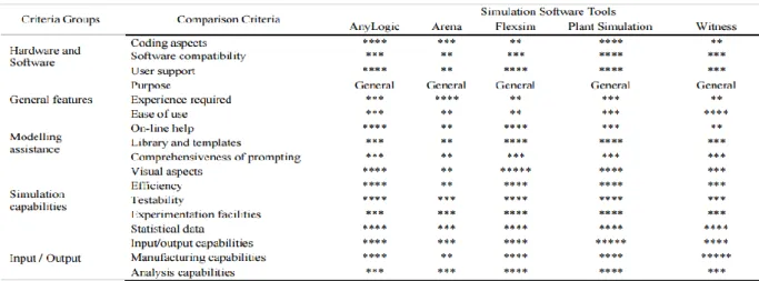
With so many upsides related to the use of simulation-based technologies in the manufactur-ing industry, there is a need to compare the various digital tools available on the market (Mourtzis, Doukas & Bernidaki, 2014). A study was made comparing five popular software systems: “AnyLogic”, “Arena”, “Flexsim”, “Plant Simulation” and “Witness”, enhancing its strengths and weaknesses. The comparison process was divided in five main categories: “Hardware and software”, “General features”, “Modelling assistance”; “Simulation capabili-ties” and “Input/Output”. The model used for the test was an adaption of a simulation model from Chryssolouris, Pierce and Dicke (1992) that studied a flexible manufacturing center. The rating scale ranges from 1 to 5 stars, being * Inadequate, **Adequate, ***Satisfactory, ****Very Satisfactory and *****Outstanding with the respective results being shown in table 1 (Mourtzis, Doukas & Bernidaki, 2014).

Table 1 - Comparison between the different available software (Mourtzis, Doukas & Bernidaki, 2014)

It can be concluded by analyzing Table 1 that 4 out of the 5 options could be considered very satisfactory on their whole, showing a wide range of capabilities for the general user.

Data types

In terms of relevant data for simulation purposes, it can be divided in 4 groups. Input data re-gards buffer capacities, process times, resources speed, while output data is related to all the statistics collected after the simulation is over. The experiment data and the internal model data represent the other two categories. They account for the simulation’s time horizon and the sub processes time, respectively. (Donhauser, Rackow, Hirschbrunn, Schudererb, & Franke, 2016).

Conclusions must be drawn only by having an accurate and precise simulator that provides accurate results. A poorly calibrated model will produce inadequate results that will end in a poor decision making process. Therefore, there is a need for model verification and valida-tion. Rabe, Spieckermann, & Wenzel (2009) recommend a model for creating and validating simulation tools with several phases, providing a structured, step-by-step guide which allows every activity to be proven and every result to be validated.

DES Case studies

Simulation modeling has been widely applied in the resolution of several improvement chal-lenges on manufacturing industries. The discrete event simulation models become relevant when there is a need to analyze a sequenced productive system, which is performed across several entities and causes the process’s state to change. This is the case of the manufacturing industry (Borshchev, 2013).

Byrne & Heavey (2006) applied a DES model to a supply chain which quantified the cost re-ductions associated with the implementation of an enhanced forecasting model and infor-mation flow. It was proven that all parties would benefit from a more active inforinfor-mation share alongside the supply chain.

Regarding the production planning field, a Chinese telecommunications manufacturer used a DES model to simulate the current plant’s situation, which faced high WIP levels (Kadipasaoglu, Xian & Khumawala, 1999). After testing the current scenario, three other sce-narios, containing slight modifications (inventory and batch sizes variations, bottleneck iden-tification), were tested. The simulation model allowed to test the impact of several production strategies that could produce both financial and operational benefits to the company.

Mendes, Ramos, Simari & Vilarinho in 2005 used a DES model alongside analytical models to allow for a production line to adapt to the current demand. Different settings could be test-ed, with the aid of the simulation tool, in order to maximize the production’s line use in dif-ferent scenarios without disrupting the line.

A DES system was created by Son, Wysk & Jones (2003) to promote the real time control of a discrete parts manufacturing plant. It was created due to the high costs of control software development and maintenance issues, and it features the first successful implementation of a real time complex control system, which was automatically generated.

DES also proves to be a valuable tool when it comes to workforce planning, as Zülch, Rot-tinger & Vollstedt analyzed in 2004. The model was used to explore the innumerous possibili-ties of schedules allocation and their respective resources. After the situation was optimized, it resulted in an enhanced organizational structure that allowed for a more competent re-assignment policy.

A simulation model was used by Roser, Nakano & Tanaka (2006) in order to test the impact that a larger capacity buffer would have on the system’s performance. The model tested sev-eral combinations that provided enough data so that the ideal buffer position within the pro-ductive line could be found.

De Ruyter, Cardew-Hall, & Hodgson (2002) displayed the potential of simulation techniques applied to the quality control department of an automotive stamping plant. The model pro-vides enough data to conclude that a low cost quality control increases the total quality cost, as many items need rework.

It can be concluded that simulation modeling, specifically DES, can be successfully applied to a wide array of fields, contemplated within the production and operations sectors of a manu-facturing plant.

In terms of the rubber production process, the following articles using some form of simula-tion were found:

Isayev, Yushanov, & Chen (1996) proposes a simulation model capable reproducing a tech-nology applicable to rubber tire recycling and other rubber wastes. The model tests how cavi-tation inside rubber particles can be used in the rubber’s devulcanization process. The created model was successfully validated by generating acceptable results when compared to the ex-perimental data gathered.

Rafei, Ghoreishy & Naderi (2009) studied how different features and parameters could influ-ence the rubber curing process, which was simulated through an advanced computational technique. Its main goal was to replicate the behavior of a thick rubber product inside the mold during the cure and post-cure stages. The created model produced accurate results when compared to experimentally measured data.

Deng & Isayev in 1991, developed a simulation model based off elements and finite-difference methods in order to tackle the challenges faced on the injection molding of rubber compounds. The study focused on two rubber compounds and their respective mechanical properties. The model’s produced outcome helped attaining the mold’s temperature, for which the properties and cycle times are optimal.

Later, a finite element simulation software was used by Felhõs, Xu, Schlarb, Váradi, & Goda (2008) to better comprehend the viscoelastic behavior of an EPDM rubber under dry rolling conditions. Through simulation, is was possible to determine the material’s viscoelasticity, as well as its behavior under strainful conditions. It proved to be a valuable tool when analyzing rubbery material’s viscoelastic properties.

2.2.4 Bottleneck analysis and theory of constrains

The bottleneck is the operation in the system that limits the production flow. This constraint affects the production rate and therefore the system efficiency itself. The material flow is af-fected, being slowed down or even stopped, as the input rate is higher than the output rate. It can be identified as the operation that keeps material waiting. The bottleneck is the weakest link on the productive chain, in terms of effectiveness and performance (Lanke, Hoseinie & Ghodrati, 2016).

It is not possible to completely remove bottlenecks from the system as, once performance is increased and constraints eliminated from one operation, the bottleneck will shift towards the new least efficient one. This will be continuously repeated (Taj & Berro, 2006).

The theory of constraints (TOC) is a structured process in which the main goal is to detect the bottlenecks on the production chain, as well as analyzing any possible interrelation between them. It started as a production planning tool and has evolved into a widespread management philosophy focused on continuous improvement, present in every sector, from production to marketing and accounting.

The main drive force behind its success was: “The Goal”, a book by Goldratt and Cox written in 1984 to inform managers about what would end up being TOC. It lays on a five step cyclic process named “The five focusing steps”, which are the following:

1-Identify the system’s constraints

2-Decide how to exploit the system’s constraints 3-Subordinate everything else to the above decision 4-Elevate the system’s constraints

5-Repeat the process

TOC is an on-going process focused on how a system is affected by its restrictions, aiming to reduce them in a continuous cycle. When correctly implemented, it brings companies benefits, such as reductions in inventory and operation expenses, while increasing production rates. The system’s production rate is defined by the production rate of the constraint operation, so in order to increase efficiency it is necessary to identify and eliminate it. That is the TOC goal which will help companies achieving their goals, thus becoming more competitive (Şimşita, Günayb, Vayvayc, 2014).

2.3 OEE indicator

The Overall Equipment Effectiveness is a performance indicator widely used in manufactur-ing industries. It is a part of the TPM (Total Productive Maintenance), which is a system fo-cused on improving the production rates mainly through preventive maintenance measures. OEE was created as an evaluation metric for TPM. It was first implemented on the semicon-ductor industry and is now used among industries with mainly automatic processes (Jeong & Phillips, 2001).

It is a powerful and simple tool that provides companies an insightful look at all the hidden production losses on their processes. This tool depends on accurate data gathering to be relia-ble. OEE is a ratio between all the time spent producing quality approved products and the scheduled time to do so. It is the result of the multiplication of three efficiency factors: Avail-ability, Performance and Quality as showed in Figure 5 (Hedman, Subramaniyan & Al-matrom, 2016). Each one of these three factors is related to 2 of 6 production losses which are the following:

1. Availability losses

1.1. Setup and adjustment time - It is also referred as planned stops and include every pe-riod of time when the equipment is ready to run but is idle. It can include setup, changeovers, cleaning, planned maintenance and inspections.

1.2. Equipment failure - Every period of time that the equipment is not able to run due to technical issues. It is also referred as downtime or unplanned stops. The main reasons account for material shortages, breakdowns and corrective maintenance (Hedman, Subramaniyan & Almatrom, 2016).

2. Performance losses

2.1. Idling and minor stops - Stoppage on the equipment that has a duration of less than two minutes and can be fixed by the operator. Product overflow and material jams, as well as misplaced machine elements can cause these losses.

2.2. Reduced speed - Every time the equipment is running slower than it was designed to. The main causes are poor maintenance, cleaning and operator inexperience (Hedman, Subramaniyan & Almatrom, 2016).

3. Quality losses

3.1. Process defects. Defective products that need to be scraped or reworked. Operator er-rors and equipment misalignment are probable causes.

3.2. Reduced yield. All the products that are produced during a stable state is reached, un-der suboptimal conditions. It includes all the scrapped parts and the ones that need rework (Hedman, Subramaniyan & Almatrom, 2016).

Figure 5 - OEE time losses overview

The availability factor is a ratio between the operating time and the loading time. The loading time is the available time to produce, excluding planned activities as breaks or planned maintenance. The operating time will account for the available time, minus the amount of time spent on unplanned and unproductive activities, such as: breakdowns, changeovers and corrective maintenance (Jeong & Phillips, 2001).

The performance indicator is the ratio between the actual production capacity and the planned production capacity. It subtracts the micro stops and low cycle times from the operating time, resulting in the net operating time. Lastly, the quality factor is a proportion between the quali-ty approved parts produced and the total amount of parts produced. The valuable operating time is the time left for quality production after all the losses are taken into consideration as it is shown on Figure 8 (Jeong & Phillips, 2001).

The OEE value will be the result of the multiplication between the three efficiency factors. The world-class goals for the discrete manufacturing industries regarding OEE factor levels are the following: Availability-90%, Performance-95%, Quality-99%. This will result in an OEE=85%. Although it is important to achieve certain numbers, one should not focus only on them, but try to implement continuous improvement strategies and increasingly more ambi-tious targets. (World-Class OEE, n.d).

3 Case study

3.1 Production policy and demand levels

ACC’s current production policy is divided in Make to Order (MTO) and Make to Stock (MTS) orders. The company is currently unable to rely solely on a MTO policy, although it is recognized to be the optimal situation.

One of the reasons for this situation to happen is the tight delivery lead times, which have been significantly reduced over the past few years due to the emergence of digital trading platforms like Amazon. In order to keep up with the competition, ACC is forced to compro-mise on delivery lead times, which are shorter than production lead times.

By doing so, production would inevitably fall behind if no stocks were maintained. With the current productive time and current accepted delivery times, there is no optimization possible that could grant an exclusively successful MTO policy.

Therefore, there is a need to rely on forecasts and maintain stocks of certain items. Production shifts between the two policies daily, in order to fill stocks and complete orders. Due to an experienced staff, production planning has achieved success by keeping up with demand. Alt-hough this will prove to be a more complicated task in the future, as demand is expected to rise, as well as reference numbers.

That is why it is vital to analyze alternatives that would enable production time extensions, and raw material to be available during the complete production expected time. It is critical to have conditions that would allow production deadlines to be met.

3.2 Production line overview

The company produces several different types of Logs, with individual requirements. These include different chemical formulas, densities, distinct raw material weight usage and differ-ent system requiremdiffer-ents.

The system requirements include all the parameters of a specific reference that will cause the production time to vary. One of these parameters is the height of the product that can range from 33’to 51’ inches, although the diameter remains constant throughout all products. Other parameters include: baking time, the number of material loads necessary to produce a single unit, EPDM usage, among others.

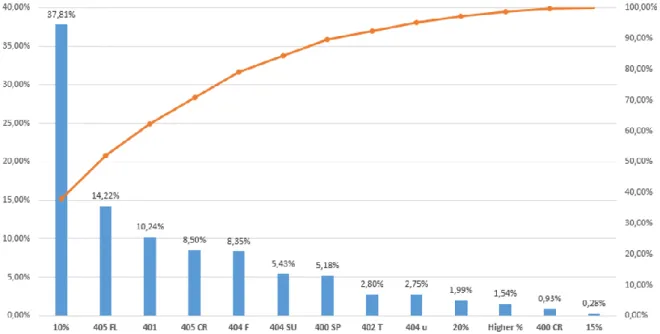
Figure 6 shows how Log production is divided by products. They were gathered in 13 main groups, each one representing a specific product. Some products have more than one size, which would increase the number of considered references to 24. These references would rep-resent 94% of all the produced items during the year 2016.

Figure 6 - 2016 Production share by reference

3.2.1 Productive process

Logs are produced exclusively during 3 to 4 straight days a week. There is only one unfazed shift enforced, with a current workforce of three experienced operators, although new person-al was being trained during the duration of the project. In order to produce Logs there is a manufacturing process involved that transforms raw material into finished product. The most important aspects of this process are have been identified and analyzed.

Raw materials

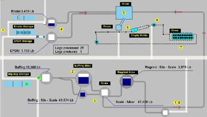
Log production requires three different raw materials displayed in Figure 7. They are stored on the adjacent hall and are transported to the room whenever they are needed and are the fol-lowing:

-Rubber buffing, which may be being colored or black. This material is kept inside Big Bags (BB) prior to be introduced in the system. It is the main raw material, which in most cases is responsible for more than 90% of the total weight of the cylinder. Black buffing is the most widely used, high quality buffing, while Colored Regrind buffing (CR) represents a material of variable color and lower quality, used in some references.

-EPDM, which are stored in pallets. Each pallet is composed of 40 plastic bags, with same

color material. This component is what grants Logs its colors. It may or not be necessary in every product and can be used in different combinations and amounts (10%-90% of the final product weight). Extra information regarding raw materials is available on Appendix B.

-Binder, which is stored in liquid containers. It acts as a glue that provides consistency to the

mixture when exposed to high temperatures.

Production Phases 1-System loading

1.1 Buffing starts flowing into the system when BB’s are hung by a hoist directly above the “Bagoff” mechanism, represented in Figure 8. The mechanism has the same function of a funnel, as it channels all the raw material towards the pipe system and into the silos. In order for material to start flowing there are some preparation operations that need to be performed by the operator. Only one bag can be used at a time. There is one separate loading station for CR and black buffing material.

1.2 Regarding the EPDM’s, the pallets have to be transported via forklift to the room, where they are stored. Then the bags of the necessary color will be discharged manually to one of the three tanks that can withhold a small volume of bags. As there is no EPDM silos, the ma-terial will flow to a scale and then it will be automatically displaced to the mixer, when need-ed.

1.3 The liquid containers keeping the binder are directly connected to the system and are re-placed when empty. There are always 2 containers on site so production is never hindered when there is a need of replacement.

Figure 8 - Bagoff equipment and EPDM tanks

2-Silos

There is a total of four available silos, two for black buffing and two for CR. Each pair has a capacity to withhold 29000 pounds, capable of keeping the approximate volume of 14 BBs of material. Each pair is connected between them and the PLC program is designed to consider each pair of silos as one. That means that material will be loaded and unloaded through both silos, of the same pair, at the same time, reducing waiting times. They will act as the produc-tion system’s buffer. Figure 9 represents the plant’s silos.

3-Scales

When material processing operations performed by the press terminate, a specific amount of material will automatically flow from the silos (or the tanks, in the EPDM case) to the scale. This amount varies from product to product. When the desired amount is reached, the connec-tion with the silos will cease and material will flow towards the mixer. After the complete load of material reaches the mixer, the Binder pump starts working, transferring the required amount to the same equipment.

4-Mixer

The mixer tank is a cylindrical equipment that will amass all of the 3 inputs, scrambling them by using centrifugal force, in order to produce a homogeneous mixture. The mixing process will last for 60 seconds and will start immediately after the binder reaches the tank. The sum of all the input weights combined will result in the load weight. If using EPDMs on a percent-age higher than 20% of the total weight, the bags will have to be loaded manually into the mixer, which is displayed in Figure 9.

Figure 9 - Silos and mixing process

5-Press

The press is responsible for the compression of the load coming from the mix tank into the mold. When the material stops falling, it will trigger the beginning of a new cycle, by allow-ing material to flow from the silos to the scales again. There are several consecutive pro-cessing operation that will occupy the press before a log is ready to move to the oven.

6-Oven

After being processed, the molds with the recently poured and compressed mix are transport-ed to the ovens to be heattransport-ed between 4 and 5 hours, depending on the product. There are two ovens with a capacity for nine molds each. This process is vital, as it is in the oven at high temperatures that the binder will have its deepest effect on the mixture, hardening it and providing enough consistency so that it will be transformed into a solid piece.

7-Demolding

The last phase of the process starts when the molds are pulled out of the oven and into the demolding station. They are transported on top of a cart which moves within a rail. In the sta-tion, the mold is separated from the finished product using a horizontal press, which extracts the material, detaching it from the mold. After the operation, the mold is placed on the same track where it will queue until needed to hold the next round of material, therefore completing a cyclic movement. The finished Logs, after being demolded will be stored in an adjacent warehouse. Figure 10 represents such operation.

Figure 10 - Oven loading and demolding operations

3.2.2 Production area constraints

While producing Logs there are several operations that occur at the same time. Some are in-dependent, and others are triggered by subsequent tasks that allow them to resume. These op-erations are grouped within one of the three sector’s areas displayed in Figure 11.

-Loading area. This area is composed by all the elements responsible for the transport, storage and deployment of all the three raw materials in the system. This section has no restriction as it is of the operators responsibility to prepare, refill and transport every empty

container when is necessary. This should be the main priority in order to keep production flowing during the longest period of time;

-Processing area. This area is composed by the press, the scales, the mixer and the system that allows for the movement and transportation of the molds between work posts. Materials can only enter the mixer when the previous load is completely deployed on the mold. When this happens materials (buffing and EPDM’s) will be transferred from the scales to the mixer. When this operation is completed binder will start flowing inwards;

-Demolding area. The operator in charge for this operation is responsible to remove the molds with material from the oven, demold it, and transport it through a rail system to the press’s proximities. It is the most physically demanding operation in the sector. The operation is dependent on the available molds ready to be pulled out of the oven, after baking. The ac-tivity will always require significant less time to complete than the press processing opera-tions. The operator’s main goal is to never let the press processing operation starve, if there are available molds. In there are not, production will stop until the resource is available again.

Figure 11 - Sector division by areas

3.2.3 Key parameters that influence production planning

When planning production one must be aware of the main parameters, inherent to each refer-ence, to maximize production rates. There is no linear dependency among them, as none fully depends on another. These parameters are the following:

1. Raw material consumption. Each reference has an exact amount of raw material needed to produce a single unit. This will influence the silos consumption rates and their production length;

2. Number of loads. Each product will have a specific amount necessary of loads to be completed. Each load will dump a predetermined amount of material into the mold; 3. Baking time. There are two default possible baking times. Usually the smaller units

will be retained in the oven less time than the bigger ones. This parameter can cause starvation due to limited amount of molds;

4. Number of molds. There are only 26 molds, and one mold can only contain one cyl-inder, regardless of its size. There has to be a careful production planning in order not to run out of molds and stall production. Although the smaller cylinders require less buffing, it will also require less time to be processed. This situation could cause the oven to be the bottleneck of the process and starve all of the following workstations; 5. Cleanout logs. Every time there is a need to change the EPDM color or combination a

cleanout log has to be created. These Logs only use black buffing and are responsible to absorb all the leftover material on the piping system from the previous series. This will eliminate color contamination between series. This products are not a resource waste, as they are marketable.

The processing time of each Log is dependent on the number of loads, material consumption and operations order. Operator’s performance can influence the production rate as well. Changeover times between series also negatively influence productivity.

3.3 Black buffing amounts deficit

The main challenge that the sector was facing occurred only when the production was di-rected towards the black buffing Logs. The raw material input rates on the system were lower than the output rates when producing the most demanded units. This situation created a deficit in available material amounts, which caused the silos, acting as buffers, to be drained at a faster rate than they could be refiled.

Eventually, production had to be readjusted on the fly to other products, including CR prod-ucts. This hindered product time deliveries and created inefficiencies by producing less urgent items to stock. The main objective of this project is to extend black buffing related production time and find solutions to improve efficiency within the sector. As a second goal, there was also a need to study how different production scenarios would affect buffing availability and production extension.

BB loading operations

Before tackling the black buffing silos usage rates problem it was mandatory to understand the prior operation, responsible to load black buffing into the system. This operation is divid-ed in the four stage representdivid-ed by Figure 12, which involve:

Stage 1 and 4 can be grouped in one single task that shall be denominated as “Transporta-tion”, representing the movements done by the hoist while loading and the unloading the bags from the system’s entry. Stage 2 accounts for the duration of time that the bag is deploying material to the system being named as the “Material Flowing” operation.

Once the bag becomes hollow, operators are responsible to proceed to change it. However they take a considerable amount of time to notice that material is no longer flowing out of the bags. The duration of this period is represented as the “Waiting” share. A complete cycle will consist on the following three phases displayed in Figure 13.

Figure 13 - Loading operations duration breakdown

Therefore, we can conclude that the material is only flowing through the system 74% of the time. This is an alarming scenario as 15% of the total time is completely wasted, impairing the production system, creating buffing shortages and reduced production lifecycles. It is be-lieved that the real waiting percentage is even higher than the one presented, as operators of-ten noticed that they were being observed and proceeded to change the bags. The transporta-tion share could only be removed if substantial investments to the productransporta-tion line were to be made.