Acidification and warming effects on a rockpool community: an experimental approach to understand stressor interactions

Acidification and warming effects on a

rockpool community: an experimental

approach to understand stressor

interactions

David Lopes Calvão

Mestrado em Ecologia, Ambiente e Território

2013/2014

Orientador

Todas as correções determinadas pelo júri, e só essas, foram efetuadas. O Presidente do Júri,

Agradecimentos

Quero agradecer ao Laboratório de Biodiversidade Costeira do CIIMAR por aceitar a minha presença nas suas instalações para poder concretizar esta tese de mestrado. Quero também agradecer ao meu orientador, Dr. Francisco Arenas, por todo o tempo dedicado e pelo apoio que me deu, por estar sempre presente quando necessitei dele, sempre com entusiasmo e paciência, e com boas ideias para ajudar a solucionar os problemas que surgissem.

Agradeço também a todos os que trabalharam comigo no Laboratório de Biodiversidade Costeira. Para além de serem bons colegas de trabalho, são também amigos, e que tornavam o dia a dia do laboratório numa experiência única. Sem eles, este ano que passou não teria sido tão bom.

Quero também agradecer à minha familia, sem eles não seria quem sou hoje. Obrigado à Diana, por me ter acompanhado na minha vida académica, obrigado à Susana pelos vários lanches partilhados ao longo do ano e obrigado a todos os meus amigos que de alguma forma me apoiaram ao longo da minha vida.

Obrigado a todos os co-autores do artigo (submetido no Journal of Experimental Marine Biology and Ecology a 24 de Setembro de 2014) pelas sugestões para o melhorar. O suporte financeiro deste projeto foi providenciado pela Fundação para a Ciência e a Tecnologia (FCT), através do projeto CLEF (PTDC/AAC-AMB/102866/2008)

Abstract

The simultaneous increase of ocean temperature and acidification caused by global climate change will have major consequences in marine ecosystems. However, community scale studies on this interaction are rare. In this study, we used mesocosms to assess the joint effects of elevated temperature and CO2 concentration on a synthetic intertidal rockpool community composed of Ulva lactuca, Chondrus crispus and Gammarus locusta. We examined the effects of both climate change related factors on some ecosystem functioning variables (i.e. biomass, photosynthetic efficiency, productivity, respiration and grazer’s mortality) using two pH levels (normal and low), three temperature levels (low, medium and high) and two grazers levels (present or absent). C. crispus, biomass increased with a higher temperature (20ºC) combined with low pH (7.9) as it did with low pH and grazer’s absence. U. lactuca’s biomass also increased with low pH, and at higher temperatures with no grazers. U.

lactuca’s photosynthetic efficiency increased with medium temperatures (17ºC). GPP

and NPP of the macroalgal assemblages increased in higher temperatures with both pH treatments. Respiration increased with increasing temperature and low pH. Low pH and high temperatures also led to an increase in mortality of G. locusta. In a future scenario of increasing temperature and CO2 concentration, rockpool communities could change due to a simultaneous decrease of potential herbivores and an increase in the biomass and functional activity of some macroalgal species.

Keywords: Climate change, warming, acidification, macroalgal assemblages, primary productivity, seaweed-grazer interaction, Ulva lactuca, Chondrus crispus, Gammarus

Resumo

O aumento em simultâneo da temperatura dos oceanos e da acidificação causada pelas alterações climáticas globais irá ter efeitos nefastos nos ecosistemas marinhos. Estudos à escala da comunidade sobre estas interações são escassos. Neste trabalho, usamos mesocosmos para compreender os efeitos conjuntos do aumento da temperatura e da concentração de CO2 numa comunidade artificial de poças de maré da zona intertidal composta por Ulva lactuca, Chondrus crispus e Gammarus locusta. Examinamos os efeitos conjunto dos factores relacionados com as alterações climáticas em algumas variáveis influentes no funcionamento do ecossistema (biomassa, eficiência fotosintética, produtividade, respiração e mortalidade de herbívoros) usando dois níveis de pH (normal e baixo), três níveis de temperatura (baixa, media e alta) e dois níveis de herbivoria (presente e ausente). Para o C.

crispus, uma temperatura elevada (20ºC) combinado com um baixo pH (7.9) levou a

um aumento de biomassa, assim como nos tratamentos com pH baixo e ausência de herbívoros. A biomassa da U. lactuca também aumentou em pH baixo e a temperaturas altas. A capacidade fotosintética da U. lactuca aumentou em temperaturas médias (17ºC). O GPP e o NPP das comunidades de macroalgas aumentaram em temperaturas mais altas em ambos os tratamentos de pH. A respiração aumentou em temperaturas elevadas e em pH baixo. pH baixo e temperaturas elevadas também levaram a um aumento da mortalidade de G. locusta. Num futuro cenário de aumento da temperatura e da concentração de CO2 , as comunidades de poças de maré podem-se alterar devido à diminuição de potenciais herbívoros simultaneamente com um aumento de biomassa e atividade funcional de algumas espécies de macroalgas.

Palavras-chave: Alterações climáticas, aquecimento, acidificação, comunidades, produtividade primária, interação alga-herbívoro, Ulva lactuca, Chondrus crispus,

Table of contents

1 – Introduction 9

2 – Material and methods 14

2.1 – Algae and animals collection 14

2.2 – Synthetic assemblage procedure 14

2.3 – Experimental setup 15

2.4 – Treatment conditions 17

2.5 – Functional responses 19

2.5.1 – Standing biomass changes 19

2.5.2 – Physiological parameters 19

2.5.3 – Functional measures: respiration and productivity 20

2.6 – Statistical analysis 21

3 – Results 22

3.1 – Biomass changes 22

3.2 – Respiration and productivity 24

3.3 – Physiological parameters 26

3.4 – Grazer’s mortality 27

4 – Discussion and conclusions 28

Lista de quadros e de figuras

Figure 1 – Change in average surface temperature (1986-2005 left and 2081-2100 right)(IPCC 2013) 9

Figure 2 - Change in ocean surface pH (1986-2005 left and 2081-2100 right) (IPCC 2013) 11

Figure 3 – Ulva lactuca (left) and Chondrus crispus (right). ( http://www.seaweed.ie/ ) 13

Figure 4 – Mesocosms inside tanks 15

Figure 5 - Schematic diagram of the experimental setup used during the mesocosm experiment 16

Figure 6 – Hourly mean temperature values of the treatments ±SE 18

Figure 7 – Hourly mean pH values of the treatments ±SE 18

Figure 8 - Mean (+SE) change of C. crispus biomass in mesocosms treated with three different temperature levels (L: low, M: medium, H:high) and two pH levels (N:normal, L:low) after 28 days of experiment. Different letters represent significant differences and same letters represent no significant differences based on on SNK

tests at p=0.05 level. 22

Figure 9- Mean (+SE) change of C. crispus biomass in mesocosms treated with pH (N: normal, L: low) and herbivores (grazers, no grazers) after 28 days of experiment. Different letters represent significant differences and same letters represent no signicant differences based on SNK tests at p=0.05 level. 23

Figure 10 - Mean (+SE) change of U. lactuca biomass in mesocosms treated with two levels of pH (N:normal, L:low)

after 28 days of experiment. Different letters represent significant differences and same letters represent no

significant differences. 23

Figure 11 - Mean (+SE) change of U. lactuca biomass in mesocosms treated with three temperature levels

(L:low, M:medium, H:high) and herbivores (grazers, no grazers) after 28 days of experiment. Different letters represent significant differences and same letters represent no significant differences based on SNK tests at p=0.05

level. 24

Figure 12 - Respiration and Net Primary Production (NPP) (mean±SE, n=48) of communities with three different

temperature levels (L: low, M:medium, H:high) and two pH levels (N:normal, L:low) after 28 days of experiment. Means with a common letter do not differ significantly from each other based on SNK tests at p=0.05 level. 25

Figure 13 - Respiration and (mean±SE, n=48) of communities with two levels of grazers (presence and absence)

after 28 days of experiment. Means with a common letter do not differ significantly from each other based on

SNK tests at p=0.05 level. 25

Figure 14 - (mean±SE, n=48) of communities with three different temperature levels (L: low, M:medium, H:high) and

two pH levels (N:normal, L:low) after 28 days of experiment. Means with a common letter do not differ significantly from each other based on SNK tests at p=0.05 level. 26

Figure 15 - Photosynthetic efficiency of U. lactuca (mean±SE, n=48) with three temperature levels (L:low, M:Medium,

H:high) after 28 days. Means with a common letter do not differ significantly from each other based on SNK tests

at p=0.05 level. 27

Figure 16 - G. locusta survival with two levels of pH (N:normal, L:low) after 28 days of experiment. Different letters

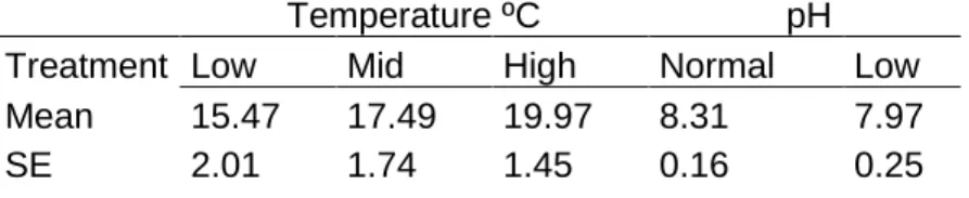
Table 1 – Treatment values (mean SE, n=8) of temperature (ºC) in mesocosms and pH in head tanks 17

Table 2 - Summary of analysis of variance for Chondrus crispus and Ulva lactuca biomass change. pH (normal and low), temperature (low, medium, high) and grazers (He) (presence and absence) are fixed factors. Significant results in

bold. 22

Table 3 - Summary of analysis of variance of Respiration, NPP and GPP of assemblages. pH (normal and low),

temperature (low, medium, high) and grazers (He) (presence and absence) are fixed factors. Significant results in bold. NPP results transformed with Ln(x+1) and GPP results transformed with Ln(x) 24

Table 4 - Summary of analysis of variance on the photosynthetic efficiency of U. lactuca and C. crispus. pH (normal and

low), temperature (low, medium, high) and grazers (He) (presence and absence) are fixed factors. Significant results in

bold. 26

Table 5 - Summary of analysis of variance of mortality of G. locusta. pH (normal and low), Ttemperature (low, medium,

1 – Introduction

Since the beginning of the industrial revolution and as a result of human activities, the atmospheric carbon dioxide (CO2) concentration rose from a pCO2 of 280 ppm to about 380 ppm in the first years of the century (Feely et al. 2004), nowadays it is close to 400 ppm (http://CO2now.org accessed 21st September 2014). CO2 is not just accumulating more and more but also rates of increase are rising (Canadella et al. 2007) and it is predicted that by the end of the century CO2 could reach up to 936 ppm with an associated drop of mean ocean pH levels (Figure 2) between 0.14 and 0.35 units (IPCC 2013). Despite, representing only a small percentage of the atmospheric gases (approximately 0.04%), CO2 is considered the major responsible of the greenhouse effect on Earth’s climate. Greenhouse effect is the phenomenon that happens when gases absorb the thermal radiation emitted by Earth’s surface and as a result the atmosphere heats up. In fact, average surface temperatures are projected to increase between 1.1ºC to 4.8ºC (Figure 1) in the next decades (IPCC 2013). While trends in temperature are somewhat variable (Lima et al. 2007), the overall warming trend is clear for virtually all parts of the Earth. Since there is a continual exchange of heat between the oceans and the atmosphere, oceans are also warming up. The average temperature of the upper layers of the ocean has increased by 0.6ºC in the past 100 years (IPCC 2013). This increase of temperature is potentially the most important change occurring in the oceans in the last centuries, as it influences physiological and ecological processes at all biological levels, from genes to ecosystems (Kordas et al. 2011). Today, it is widely accepted that human activities are causing these environmental changes (IPCC 2013), and that they have a high ecological impact on natural systems (Halpern et al. 2008). This impact is changing the global biodiversity at unprecedented rates (Dobson 2005).

CO2 in the atmosphere is also being incorporated into the oceans because it is highly soluble in water. The upper layer of the oceans is the zone of main exchange of carbon with the atmosphere. The capacity to take up CO2 is controlled by the reaction of CO2 with the carbonate ion to form bicarbonate (HCO3-). CO2 reacts with water to produce carbonic acid (H2CO3). Carbonic acid then dissociates, and produces a hydrogen ion and a bicarbonate ion. This chemical balance is in equilibrium according to the next equation:

CO2 + H2O ↔ HCO3- + H+ HCO3- ↔ CO32- + H+

So, if CO2 is removed from the water, more carbonic acid and bicarbonate will be produced, until equilibrium is reached. These reactions are known as the Seawater Carbonate System (SWCS) (Pearson & Palmer 2000; Barry et al. 2010). Thus, the increase in the atmospheric CO2 concentration, due to the human fossil fuel combustion and deforestation, will result in an increase of CO2 concentration in seawater. Consequently there will be changes in the SWCS, leading to a decrease in seawater pH (Hale et al. 2011). This pH drop is commonly known as ocean acidification. Ocean acidification is a threat to marine ecosystems, since it affects the calcification processes of several organisms that could alter the community structure and biodiversity in marine benthic communities (Hofmann et al. 2012). Previous studies that investigated the responses of calcifying organisms to altered seawater carbonate chemistry have shown that acidification is endangering several marine ecosystems leading to dissolution of coral skeletons (Fine & Tchernov 2007), reducing rates of reef calcification (Langdon et al. 2000) and diminishing shellfish calcification (Gazeau et al. 2007). Calcified structures usually provide protection, so with the modification of their ability to produce these structures, they will need to adapt to the new seawater chemistry, change their distribution to a region that suits them better or suffer with the negative impact of the reduced calcification. Kelp forests are also in danger, since the number of kelp recruits is affected by the increase of turf forming algae, and these are predicted to increase with climate change (Connell & Russell 2010).

Figure 2 – Change in ocean surface pH (1986-2005 left and 2081-2100 right) (IPCC 2013)

The combined effect of increasing CO2 concentrations and temperature on organisms and ecosystems may be greater than the impact of CO2 or temperature alone (Rodolfo-Metalpa et al. 2011; Martin et al. 2008; Crain et al. 2008). One example of this is an experiment in CO2 vents in the Mediterranean Sea, showing that some calcifying species were more vulnerable to the effects of ocean acidification at warmer seawater temperatures (Rodolfo-Metalpa et al. 2011). Differences in the sensitivity of macroalgae to ocean acidification can alter completely coastal ecosystems as changes in algal communities may lead to differences in herbivore diversity and abundance (Benedetti-cecchi 2001). These changes in the species distributions and abundances are expected to expand to all trophic levels of marine food webs (Fabry et al. 2008). Humans are dependent on ocean ecosystems for their valuable goods and services, especially coastal areas (Barbier et al. 2011) Therefore, any dramatic change in the coastal community structure and biodiversity might have long lasting consequences in the functioning of marine ecosystems with unpredictable implications to human welfare (Harley et al. 2006).

The intertidal habitat is a transitional zone that has a diverse array of unique ecosystems wherever land and the ocean meet. The rocky intertidal is the product of marine erosion, and it is the most primitive type of coast because it has been altered the least. The region of the seashore is bounded on one side by the height of high tide and on the other by the height of low tide. In the rocky intertidal, rockpools are a dynamic ecosystem that changes drastically during an entire day due to the tides. During high tide, rock pools are completely submerged, water is in constant circulation and it becomes an open system. During low tide, the rock pool becomes a closed system and is isolated from the ocean. During low tide, the upper water layers are exposed to air, undergoing temperature fluctuations, intense solar radiation and also desiccation due to water evaporation. When there’s rain, salinity may decrease due to the freshwater income. If there is enough algal growth within the rockpool, oxygen will

be high during the day, but low at night, something that rarely occurs in the open sea. Therefore, organisms dwelling in rockpools are subjected to great fluctuations of temperature, salinity and pH (Valentine et al. 2007). For life to occur in rockpools, it must be able to withstand these fluctuations.

A fundamental process in nature is the ability to acquire energy. This happens by moving energy from the Sun to the food chain. Plants harness sunlight, in a process known as primary production, and then the energy flows through the food chain. This leads to species interacting with each other to obtain the essential resources needed to survive. One of these interactions is the herbivore-plant interaction. Grazers interact with plants by consuming them, and this top-down control regulates the abundance of plants in an ecosystem (O’Connor 2009). Due to their sensitivity to disturbances in their ecosystems and because their grazing capacity, amphipods are often selected for ecological studies (Neuparth et al. 2002). Gammarus locusta (Linnaeus, 1758) is an amphipod species that is widely distributed along the North-East Atlantic, with a range that has its southern limit in the Mediterranean Sea (Costa & Costa 1999). It is found in different substrates, and appears on the medium to low intertidal zone. It is an omnivore, feeding on macroalgae, and on sediment detritus (Costa et al. 1998).

Portugal’s continental coast is included within the South European Atlantic Shelf ecoregion, where there are coincidental distributions of macroalgal species of both boreal and Lusitanian origins (Tuya et al. 2012). A large number of cold- and warm-water marine species have their distributional range edges (northern or southern) along this coastline, while other species display latitudinal clines in abundance (Lima et al. 2007).

In our study we focused on two co-occuring rocky intertidal macroalgae: Ulva lactuca (Linnaeus, 1753) and Chondrus crispus (Stackhouse 1797) (Figure 3). These two species are very abundant in Portugal’s coastline. U. lactuca is a green alga that largely colonizes tide-pools. It grows from a discoid holdfast, attached to rocks or other algae. It is distributed all over the world. C. crispus is a red alga that colonizes rocky shores. It is distributed along the coasts of the Northern Atlantic.

Figure 3 – Ulva lactuca (left) and Chondrus crispus (right). (http://www.seaweed.ie/)

Several experiments have tried to predict the impact of climate change on different algae. Some studies tried to find the responses of U. lactuca and C. crispus to ocean acidification, and concluded that elevated CO2 concentrations (i.e. low pH) caused a significant increase in biomass (Olischläger et al. 2013). However the opposite effect was found on calcifying species, like the reduced calcification of Corallina officinalis (Hofmann et al. 2012). On other studies, temperature was the factor studied, showing that increasing temperature has a negative impact on algae like Laminaria ochroleuca (Biskup et al. 2014). Most of the studies have only focused on one factor, or those that had multiple factors often used only one species, instead of a community.

The present work studies the joint effects of rising temperature and acidification on biomass change, productivity and healthiness of two abundant rocky intertidal macroalgae Ulva lactuca and Chondrus crispus. Furthermore we test the combined effects of temperature and acidification on herbivore-macroalgae interactions using these two algae and one common rocky intertidal consumer, the grazing amphipod

Gammarus locusta. To examine the performance of a rockpool macroalgal assemblage

facing anthropogenically related climate change factors, we mimick a rocky intertidal ecosystem by constructing a set of mesocosm tanks harbouring the three species.

2 – Materials and Methods

2.1 – Algae and animals collection

All the seaweeds used in our experiments were gathered at Praia Norte (Viana do Castelo 41º 69’ N, 8º 85’ W), at the 14th _{and 16}th _{of April 2014, during the spring low} tide. On that date individual fronds of Chondrus crispus Stackhouse 1797, Ulva lactuca Linnaeus 1753 and boulders holding turf species (mostly Corallina officinalis Linnaeus 1758) were collected and transported to CIIMAR (Centro de Investigação Interdisciplinar Marinha e Ambiental da Universidade do Porto) in cold boxes in less than 2 hours. Once at the laboratory, seaweeds were rinsed with fresh water to remove herbivores. After washing, they were placed outdoors in a 300 litres seawater tank with temperature (14º C) controlled provided by a seawater chiller (Teco® TR20). Boulders containing turf species were cut into pieces using a stone cutter to fit in the mesocosms used in this experiment (stone volume between 100 and 150 cm3), always selecting those areas with maximum cover of turf.

Dozens of Gammarus locusta were captured from a tank with Laminaria ochroleuca located in an aquaculture facility in Póvoa de Varzim. They were transported to CIIMAR in cold boxes in less than 1 hour. They were placed in a plastic aquarium (20dm3) with controlled temperature (15ºC). Water was replaced every 3 days. The animals where fed every day with Ulva lactuca.

2.2 – Synthetic assemblage procedure

We used synthetic macroalgal assemblages to carry out our experiment. The assemblages were constructed using a fiber glass mesh that held together the stone with the turf assemblage and fronds of Chondrus crispus and Ulva lactuca. We used C.

crispus fronds with an average weight of 4.1g±7.0 (mean±SE, n=48), and U. lactuca

fronds with an average weight of 3.5g±1.5 (mean±SE, n=48). Every single weight was recorded. Synthetic assemblages were identified with a plastic label and a cable tie. C.

crispus fronds were fixated to the rock with a small cable tie, clasping both cable ties to

using a plastic peg. The macroalgal assemblages were placed inside the experimental mesocosms (open acrylic cylinders, see below), and then placed in larger tanks corresponding with their respective treatment. After that, U. lactuca was placed inside

the cylinder, remaining free in the water column. Lastly, 2 G. locusta were placed in each mesocosm.

The experiment was performed in a mesocosm placed in an outdoor area, from April until May 2014, lasting for 28 days.

2.3 – Experimental setup

Each macroalgal assemblage (fronds of U. lactuca, C. crispus and algal turf) was allocated in a 2.5 dm3 acrylic open cylinder (10cm x 33cm). The cylinders (8 per tank) were submerged in six tanks (40cm x 50cm x 35cm, 70dm3), where temperature and pH were controlled, and fixed vertically using a plastic net, (see Figure 3). At the bottom end of each cylinder, a 1mm fiberglass mesh was placed to prevent that the algae and the animals escaped from the mesocosms. We placed a water pump (Eheim 1000) underneath each cylinder to enhance the water flow. Mesocosms were covered by a neutral fiberglass mesh to reduce in 30% the light intensity. This way the effects of the excess of light were prevented, due to the fact that the tanks were white and placed outdoors.

In order to prevent large changes in water temperature due to heat exchanges with the air, the tanks (64 litres) that contained the mesocosms with the assemblages were submerged in a water bath created by 300 litres tanks. Water temperature was regulated using heaters (titanium heaters) and seawater chillers simultaneously (Aqua Medic® Titan 2000) controlled electronically using a microprocessor controller (Aqua Medic® AT Control System) with temperature sensors.

We used two head tanks (1000 litres) adjacent to the mesocosms to create the pH treatments. In those tanks sea water pH was regulated using individual pH probes connected to the Aqua Medic AT Control System that controlled solenoid valves connected to a CO2 bottle. In the low pH tank, CO2 was burbled in order to maintain a pH of 7.7. To reduce CO2 flux from the CO2 bottle to the tank and to prevent rapid changes in pH we used a rotameter (Aalborg®)

Water from the head tanks flowed to the six experimental tanks where the mesocosm were submerged. Every 12 hours, water from each treatment tank was completely renovated, mimicking the water entering the intertidal pools during the high tide. This renovation took 2 hours. Using water pumps (Oceanrunner OR1200), water was lead into each treatment from its respective water deposit (normal pH deposit and 7.7 pH deposit).

Figure 5 - Schematic diagram of the experimental setup used during the mesocosm experiment. In yellow are

To prevent nutrient limitation, every two days NaNO3 and NaH3PO4 was added until a final concentration of 50 µM of N and 5 µM of P was achieved.

2.4 – Treatment conditions

The goal of the experiment was to examine how climate change related environmental drivers, temperature and pH, may shape the interaction between grazers and primary producers. Thus, three treatments were included in the experiments: (1) water temperature, with three levels (low 14.47ºC± 2.01, medium 17.49ºC±1.74 and high 19.97ºC±1.45; (2) water pH, with two levels (normal pH 8.31±0.16 and low pH 7.97±0.25; (3) herbivore (Gammarus locusta) presence or absence (Figure 5). pH and temperature levels were selected based on predictions for the end of the century (IPCC 2013). Each treatment combination was replicated four times. Thus we used a total of 48 mesocosms in the experiment. During the day, temperatures varied according to Figure 5. For the acidification treatments, the pH values varied as seen in Figure 6.

Table 1 – Treatment values (mean SE, n=8) of temperature (ºC) in mesocosms and pH in head tanks

Temperature ºC pH

Treatment Low Mid High Normal Low Mean 15.47 17.49 19.97 8.31 7.97

13 14 15 16 17 18 19 20 21 22 23 0 3 6 9 12 15 18 21 24 T emp er atu re (Cº) Time (h) Low Mid High

Figure 6 – Hourly mean temperature values of the treatments ±SE

Figure 7 – Hourly mean pH values of the treatments ±SE

7,6 7,7 7,8 7,9 8 8,1 8,2 8,3 8,4 8,5 8,6 0 3 6 9 12 15 18 21 24 pH Time (h) pH N pH L

2.5 – Functional responses

2.5.1 – Biomass changes

Fresh weight of each algal frond was recorded at the beginning of the experiment, and then again 28 days later at the end of the experiment. Biomass change was calculated using the following formula:

FWf / FW0

where FWf is the fresh weight in grams at the end of the experiment and FW0 is the fresh weight in grams at the end of the experiment.

At the end of the experiment, all fronds were rinsed with fresh water to remove salt. Using a scalpel, the algae in the boulders were scrapped. Subsequently, the algae were dried at 50ºC for 48 hours, and then the dry weights were determined in order to adjust data to biomass.

2.5.2 – Physiological variables

The algae physiological status was assessed through the photosynthetic capacity of their photosystem II, also known as Maximal Quantum Yield of Photosynthesis. The principle behind this assessment is that light that is absorbed by chlorophyll molecules can meet one of three fates: being used in photosynthesis (photochemistry), being dissipated as thermal energy or being re-emitted as light (chlorophyll fluorescence). These processes compete with each other, so when there is an increase in the efficiency of one of them, the yield of the other two will have a decrease. Using this competition between the processes, information about changes in the efficiency of photochemistry and heat dissipation can be obtained by measuring the yield of chlorophyll fluorescence. By exposing a frond of a darkness adapted algae to a defined wavelength light, and measuring the amount of light re-emitted at longer wavelengths, the fluorescence yield can be assessed (Maxwell & Johnson 2000).

Each individual’s photosynthetic capacity was measured using a mini-PAM (pulse amplitude modulated) (Walz) chlorophyll fluorometer. Each frond was placed in a black box (in order to prevent any external light input) and submerged in its treatment’s respective water. There was a waiting time in the dark of 30 minutes so that the algae

adapted to darkness. After that, the chlorophyll fluorometer measured the fluorescence in the dark (F0) and the maximum fluorescence (Fm). Using these values, the Maximal Quantum Yield of Photosynthesis was calculated, according to the next equation:

Fv/Fm = (Fm – F0)/Fm

where Fv is the variable fluorescence (or the difference between Fm and F0). The Fv/Fm determines the maximum efficiency of the photochemical energy conversion in a darkness adapted plant (Maxwell 2000).

2.5.3 – Respiration & Primary productivity

Assemblages’ functional measures, i.e. respiration, net, net primary productivity (NPP) and gross primary productivity (GPP) were estimated through the determination of the dissolved O2 fluxes in incubations at seven different light intensities. We used the 2.5 dm3 acrylic cylinders to incubate our assemblages in an incubator provided with fluorescent lamps (30W Osram Biolux®). Each assemblage was exposed to seven consecutive light intensities (0, 24, 164, 262, 345, 417 and 1578 μmol m-2 _s-1_{). pH and} temperature treatment conditions were controlled as in the experimental setup using by the AT Control system and coolers. Changes in the O2 concentrations were recorded every 30 seconds by luminescent oxygen probes connected to a data logger (HQ40D Hach Lang) and placed in each incubation chamber. Each light cycle lasted for 20 minutes, after which the next sets of lights were turned on. Respiration and productivity were estimated for each irradiance level through the measurement of oxygen fluxes by regressing oxygen concentration in the chamber (measured in μmol) through time (s–1_). Fluxes were corrected by seawater volume inside the cylinder and assemblages biomass. To prevent the influence on the productivity and respiration of microalgae in the treatments, all the seawater used was filtered (5µm).

Three ecosystem functioning surrogates were determined per assemblage: (1) maximum net primary productivity (max NPP), the maximum productivity (i.e. maximum slope for the oxygen concentration versus time relationship) recorded at any light intensity (μmol O2 s–1); (2) assemblage respiration, the oxygen consumption during the dark period of the incubation (μmol O2 s–1); and (3) maximum gross primary productivity as the sum of the two previous variables, i.e. maximum NPP+|Respiration|.

2.6 – Statistical analysis

Changes in biomass, primary productivity and physiological parameters were assessed using a 3-factor orthogonal analysis of variance (ANOVA). The factors were temperature (3 levels: low, medium, high), pH (2 levels: natural and low) and grazers (2 levels: presence and absence). All factors were fixed. A posteriori multiple comparisons were done using Student-Newman-Keul’s (SNK) tests (p > 0.05). The homogeneity of variances was evaluated by using Cochran’s test and data was transformed using ln(x+1) when necessary. Univariate statistical analyses were performed with WinGMAV 5.0 (EICC, The University of Sidney)

3 – Results

3.1 – Standing biomass changes

The analysis of variance for Chondrus crispus and Ulva lactuca biomass changes is presented in Table 2. Biomass changes of C. crispus and U. lactuca over time (28 days) are shown in the next Figures. C. crispus biomass increased in all treatments, and this increase was influenced by temperature, pH (Figure 7) and the presence of grazers (Figure 8). C. crispus biomass increased significantly with temperature (table 2), but this change was not consistent with pH treatments (significant pH x Te interaction; p < 0.01, table 2). The increase in C. crispus biomass with high temperature was significant only when low pH was also applied (7). Corallina officinalis data was not used due a bleaching effect that occurred in all treatments.

Table 2 - Summary of analysis of variance for Chondrus crispus and Ulva lactuca biomass change. pH (normal and

low), temperature (low, medium, high) and grazers (He) (presence and absence) are fixed factors. Significant results in bold.

Figure 8 - Mean (+SE) change of C. crispus biomass in mesocosms treated with three different temperature levels (L:

low, M:medium, H:high) and two pH levels (N:normal, L:low) after 28 days of experiment. Different letters represent significant differences and same letters represent no significant differences based on on SNK tests at p=0.05 level.

C. Crispus U. Lactuca DF F p DF F p pH 1 1.37 0.2492 1 4.31 0.0452 Temperature (Te) 2 11.45 0.0001 2 1.19 0.3157 Herbivore (He) 1 0.3 0.5897 1 2.33 0.1353 pHXTe 2 6.75 0.0032 2 1.03 0.3680 pHXHe 1 5.35 0.0265 1 2.18 0.1487 TeXHe 2 1.11 0.3404 2 5.29 0.0097 pHXTeXHe 2 1.56 0.2247 2 1.76 0.1858 a _a a a ab c 0,0 0,5 1,0 1,5 2,0 2,5 L M H Bio mass chan g e Temperature

C. crispus

C. crispus biomass was significantly affected by the presence of grazers, but this

pattern was not consistent over pH treatments (significant pH x He interaction; p < 0.05, Table 2). The change in biomass was significantly higher in those mesocosms with no grazers and low pH (Figure 8)

Figure 9- Mean (+SE) change of C. crispus biomass in mesocosms treated with pH (N: normal, L: low) and herbivores

(grazers, no grazers) after 28 days of experiment. Different letters represent significant differences and same letters represent no signicant differences based on SNK tests at p=0.05 level.

U. lactuca biomass increased significantly with low pH conditions (Table 2, Figure 9). U. lactuca biomass showed a significant change with temperature variation and the

presence of grazers (i.e., significant Te x He interaction; p > 0.01, Table 2). U. lactuca biomass was significantly higher with high temperatures and no grazers (Figure 10). No change in biomass was found in those mesocosms with grazers (Figure 10).

Figure 10 - Mean (+SE) change of U. lactuca biomass in mesocosms treated with two levels of pH (N:normal, L:low)

after 28 days of experiment. Different letters represent significant differences and same letters represent no significant differences. ab a ab b 1,3 1,35 1,4 1,45 1,5 1,55 1,6 1,65 1,7 1,75 1,8 pH N pH L Bio mass chan g e

C. crispus

U. lactuca

Figure 11 - Mean (+SE) change of U. lactuca biomass in mesocosms treated with three temperature levels (L:low,

M:medium, H:high) and herbivores (grazers, no grazers) after 28 days of experiment. Different letters represent significant differences and same letters represent no significant differences based on SNK tests at p=0.05 level.

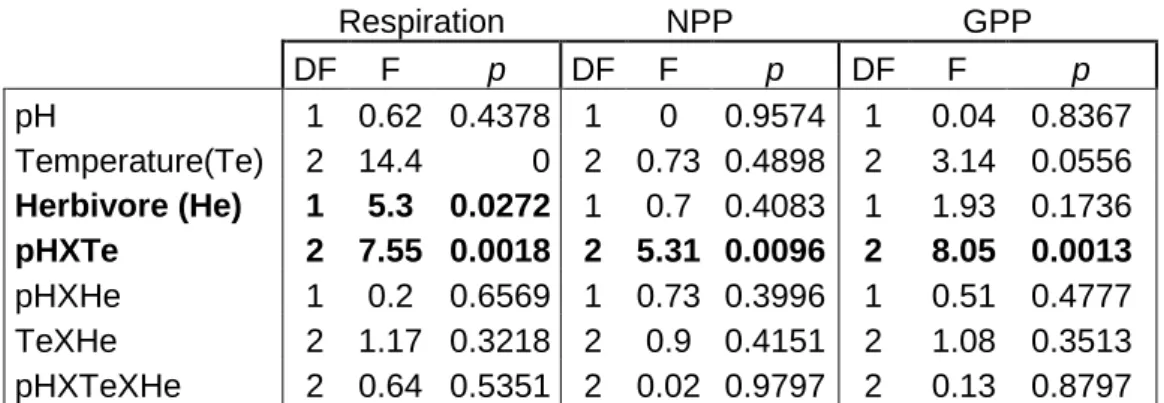
3.2 – Functional measures: productivity and respiration

The analyses of variance for the functional measurements indicated significant and interactive effects of pH and temperature in the productivity and respiration of the assemblages (Table 3). Respiration in the macroalgal assemblages increased with low pH and high temperature treatments (Figure 11) In the normal pH treatments, medium temperature led to an increase in NPP, and in the low pH there were no significant differences between treatments (Figure 11). The presence of grazers had a significant effect on the respiration of the macroalgal assemblage (Table 3).

Table 3 - Summary of analysis of variance for Respiration, NPP and GPP of macroalgal assemblages. pH (normal and

low), temperature (low, medium, high) and grazers (He) (presence and absence) are fixed factors. Significant results in bold. NPP results transformed with Ln(x+1) and GPP results transformed with Ln(x)

Respiration NPP GPP DF F p DF F p DF F p pH 1 0.62 0.4378 1 0 0.9574 1 0.04 0.8367 Temperature(Te) 2 14.4 0 2 0.73 0.4898 2 3.14 0.0556 Herbivore (He) 1 5.3 0.0272 1 0.7 0.4083 1 1.93 0.1736 pHXTe 2 7.55 0.0018 2 5.31 0.0096 2 8.05 0.0013 pHXHe 1 0.2 0.6569 1 0.73 0.3996 1 0.51 0.4777 TeXHe 2 1.17 0.3218 2 0.9 0.4151 2 1.08 0.3513 pHXTeXHe 2 0.64 0.5351 2 0.02 0.9797 2 0.13 0.8797 a ab b a a a 0 1 2 3 4 5 L M H Bio mass chan g e Temperature

U. lactuca

a b a a a a 0,0 0,2 0,4 0,6 0,8 1,0 1,2 1,4 1,6 1,8 L M H NP P (g O 2 DW g -1 hr -1) Temperature pH N pH L

Figure 12 - Net primary production (NPP) and respiration and (mean±SE, n=48) of assemblages with three different

temperature levels (L: low, M: medium, H:high) and two pH levels (N:normal, L:low) after 28 days of experiment. Means with a common letter do not differ significantly from each other based on SNK tests at p=0.05 level.

Figure 13 - Respiration (mean±SE, n=48) of macroalgal assemblages with two levels of grazers (presence and

absence) after 28 days of experiment. Means with a common letter do not differ significantly from each other based on SNK tests at p=0.05 level.

Regarding gross primary production (GPP), there was a significant increase in GPP in normal pH and medium temperature conditions (Figure 14). Similarly, a significant increase in GPP was found in low pH and high temperature conditions (Figure 13)

a b b b ab c -1,8 -1,6 -1,4 -1,2 -1,0 -0,8 -0,6 -0,4 -0,2 0,0 L M H Re s pir a tion (g O 2 DW g -1 hr -1) pH N pH L a b -1,2 -1,0 -0,8 -0,6 -0,4 -0,2 0,0 Grazers No Grazers Respir atio n (g O 2 DW g -1 hr -1)

a b ab ab a b 0,0 0,5 1,0 1,5 2,0 2,5 3,0 3,5 L M H G P P (g O 2 m -2 hr -1) Temperature pH N pH L

Figure 14 - (mean±SE, n=48) of communities with three different temperature levels (L: low, M: medium, H:high) and

two pH levels (N:normal, L:low) after 28 days of experiment. Means with a common letter do not differ significantly from each other based on SNK tests at p=0.05 level..

3.3 – Physiological variables

Temperature was the only factor with a significant effect on U. lactuca‘s photosynthetic activity (Table 4). Thus, medium temperature showed a significant increase in photosynthetic efficiency compared to low and high temperatures (Figure 14). C.

crispus did not show a significant change in Fv/Fm at the end of the experiment.

Table 4 - Summary of analysis of variance on the photosynthetic efficiency of U. lactuca and C. crispus. pH (normal and

low), temperature (low, medium, high) and grazers (He) (presence and absence) are fixed factors. Significant results in bold. U. Lactuca C. Crispus DF F p DF F p pH 1 0.97 0.3318 1 0.52 0.4744 Temperature(Te) 2 7.06 0.0026 2 1.1 0.3454 Herbivore (He) 1 0.1 0.7502 1 0.22 0.6389 pHXTe 2 1.58 0.2191 2 2.21 0.1247 pHXHe 1 1.43 0.239 1 0.32 0.5775 TeXHe 2 0.59 0.5601 2 2.23 0.1216 pHXTeXHe 2 0.96 0.393 2 0.04 0.9638

a a a b ab ac 0 0,5 1 1,5 2 2,5 L M H Nu mb er of G raz er s Temperature pH N pH L a b a 0,0 0,1 0,2 0,3 0,4 0,5 0,6 0,7 L M H F v /Fm Temperature

Figure 15 - Photosynthetic efficiency of U. lactuca (mean±SE, n=48) with three temperature levels (L:low, M:Medium,

H:high)after 28 days. Means with a common letter do not differ significantly from each other based on SNK tests at p=0.05 level.

3.4 – Grazer’s mortality

Every cylinder with the herbivore treatment started with 2 animals, and at the end of the experiment we checked for grazer’s mortality. Both temperature and pH had a significant effect on the survivability of G. locusta (Table 5). Mortality was no significantly different among temperatures with a normal pH level (Figure 15). However, with low pH, there is a significantly higher mortality with increasing temperatures (Figure 15).

Table 5 - Summary of analysis of variance of mortality of G. locusta. pH (normal and low), Ttemperature (low, medium,

high) and grazers (He) (presence and absence) are fixed factors. Significant results in bold.

DF F p

pH 1 0.13 0.7222

Temperature(Te) 2 5.09 0.0177

pHXTe 2 5.61 0.0128

Figure 16 - G. locusta survival with two levels of pH (N:normal, L:low) after 28 days of experiment. Different letters

4 – Discussion and Conclusions

Interactive effects of seawater temperature, pH and herbivores on the biomass of Ulva

lactuca and Chondrus crispus were revealed on this study. Results suggested that on

overall an increase of temperature and a decrease of pH have a positive effect on the biomass of both macroalgae.

In our experiments, the biomass of C. crispus rose under elevated temperature and low pH. Similarly, Hofmann et al. (2012) used macroalgal communities of Corallina

officinalis, Chondrus crispus, Polysiphonia fucoides, Dumontia incrassata and a few

other macroalgal species to assess the competition between calcifying and non-calcifying algae under elevated CO2 concentrations. They used 3 different pH treatments (8.22, 8.05 and 7.73). The calcifying C. officinalis had a decrease in growth rates, but C. crispus cover increased in low pH conditions, as it did in our study. These results indicate that an increase of CO2 concentrations in the future might lead to a structural change of intertidal macroalgae communities, namely the decrease in abundance of calcifying algae like Corallina spp. and the increase of C. crispus cover. Likewise, the biomass of U. lactuca increased with low pH conditions in our experiment. However, warmer temperatures increased the biomass of U. lactuca only when grazers were not present in the mesocosm. This could mean that in a future seawater scenario of increasing temperature and low pH, U. lactuca can increase its biomass faster than in the present day conditions. In another study, Olischläger et al. (2013) used 2 pH levels (preindustrial scenario and future scenario) to determine the effects of ocean acidification on U. lactuca. Similar to our results, they asserted that the biomass of U. lactuca increased with higher CO2 concentration treatments. These results suggest that in habitats with limited carbon supply (like rockpools), U. lactuca might be a better colonizer of new rockpools, although this might negatively affect to other species present in such habitats due to a high consumption of inorganic carbon by U. lactuca.

The aforementioned studies did not use temperature as a factor. Therefore, they are not able to predict what will be the joint influence of seawater warming and acidification on these species, whether it potentiates the negative or positive effects, or whether it has no impact at all. It seems that U. lactuca response to stress conditions will be more dependent on the presence of grazers feeding on the algae than C. crispus. There

were no significant results for the effect of any of the climate change factors on the physiological status (in terms of photosynthetic activity, Fv/Fm) of C. crispus. However, the photosynthetic activity of U. lactuca was significantly affected by an increase in temperature. On the medium temperature treatment there was a higher Fv/Fm than on the other two temperature treatments.

We found interactive effects of temperature and pH on the respiration and productivity of the macroalgal assemblages. Thus, respiration in the macroalgal assemblage increased significantly in low pH conditions and increasing temperature; meanwhile respiration did not change in normal pH conditions when temperature increased. Temperature and pH also had an effect on the amount of O2 produced, with an increase in GPP as temperature and acidity increased. There was an increase of O2 production in medium temperatures and normal pH for NPP. In low pH treatments, there were no significant differences. This raises the question of how O2 production would be with increasing levels of temperature and pH. A recent study by Olabarria et al. (2013) combined both temperature and acidification. In this study, the authors also used macroalgal communities from rockpools, and successfully analyzed the effects of the two climate change variables at the individual and community level. They concluded that temperature and CO2 had a significant effect on community performance (GPP and respiration), and that the biomass of some algal species suffered significant losses at lower pH and higher temperatures.

G. locusta’s mortality did not change significantly across temperatures with a normal

pH. However, in low pH conditions, mortality increased with increasing temperature. Hale et al. (2011) assessed the joint effects of both high temperature and high acidity in a marine invertebrate community. These stressors led to changes in the species’ abundance and diversity, and the number of arthropod species was negatively affected by temperature, pH and the interaction between both factors. The same result was obtained in our study, where the survival of G. locusta was affected by the interaction of both pH and temperature. Their work also shed light on how it is unlikely to find a generic response model for both reduced pH and elevated temperature on a community based only on each species response to climate change. Therefore it is important to use multilevel community studies in order to determine realistic responses of macroalgal assemblages’ to climate change.

These studies and our results demonstrated the combination of different responses that organisms and communities from coastal marine ecosystems can have regarding climate change. Our study tried to go a step further by adding herbivores to the

community. One of the results obtained was that their survivability was tied to the interaction between pH and temperature. The decrease of grazers due to climate change might have a direct effect on the coastal community. Moreover, if climate changes variables, such as pH and/or temperature can enhance the algal growth of some macroalgal species, and at the same time decrease the abundance of potential consumers, the marine plant-herbivore interaction can be completely affected. Without a proper top-down regulation, some macroalgal species could grow faster than others. Both C. crispus and U. lactuca had a greater increase of biomass when grazers were absent. This result means that with increasing temperatures and CO2 concentrations, macroalgal communities like the ones we studied here, might stop having a top-bottom regulation due to the disappearance of herbivores. This can lead to an overall increase in algal biomass, both caused by the lack of herbivore control and by the increase of CO2 concentration in a future scenario of climate change. Consequently, this can change the light conditions (Alsterberg et al. 2013), the nutrient availability (Falkenberg et al. 2013) or the productivity (Anthony et al. 2008) of the entire coastal ecosystem. There is an urgent need for community oriented approaches to test the factors that control interactions between different species. However, short-term experiments are not able to show the effects of a continuous exposure to global warming (Olabarria et al. 2013),due to the fact that it is only a small window of time, and macroalgae might adapt to this exposure (Hurd et al. 2009). Research based on the combined effects of different climate change variables on macroalgal assemblages can provide with a better understanding of the process of physiological adaptation of the macroalgal community in coastal ecosystems

Climate change is causing global warming and ocean acidification with consequent effects on marine fauna and flora worldwide (IPCC 2013). Our results revealed the interactive effects of temperature and acidification on U. lactuca, C. crispus and G.

locusta. Our work has shed some light of how macroalgal assemblages and marine

plant-herbivore interactions can be affected by anthropogenically induced climate change. In a future scenario of global change, macroalgal species will have to adapt to the new conditions, change their distribution, or disappear (Kordas,et al. 2011). Thus, the responses to increases in temperature and ocean acidification explored here have implications for several changes in the structure and functioning of macroalgal assemblages.

Future research should focus on entire communities of interacting species to predict the impacts of ocean warming and acidification on coastal marine ecosystems. The impacts of climate stressors will depend on both community adaptability to the new climate challenges, and the traits that affect the strength of interaction between species (Poore et al. 2013; Morelissen & Harley 2007). Climate change stressors and synergistic effects of the multiple environmental drivers involved led to nonlinear responses of organisms. This hinders our ability to predict the consequences of climate change. Mechanistic experimental approaches considering simultaneous multiple stressors and several levels per stressors are probably a good way to understand the full consequences of climate change (Crain et al. 2008). Further research is needed to understand how herbivore preferences among macroalgal species could be affected by climatic stress conditions, and how herbivores may adapt to those altered conditions.

5 – References

Alsterberg, C. et al., 2013. Consumers mediate the effects of experimental ocean acidification and warming on primary producers. Proc Natl Acad Sci U S A, 110(21), pp.8603–8608.

Anthony, K.R.N. et al., 2008. Ocean acidification causes bleaching and productivity loss in coral reef builders. Proceedings of the National Academy of Sciences of

the United States of America, 105(45), pp.17442–6.

Barbier, E.B. et al., 2011. The value of estuarine and coastal ecosystem services. Barry, J. et al., 2010. Atmospheric CO2 targets for ocean acidification perturbation

experiments. Best Practices for Ocean Acidification Research, pp.53–66. Benedetti-cecchi, L., 2001. Variability in abundance of algae and invertebrates at

different spatial scales on rocky sea shores. Marine ecology. Progress series, 215(Levin 1992), pp.79–92.

Biskup, S. et al., 2014. Functional responses of juvenile kelps, Laminaria ochroleuca and Saccorhiza polyschides, to increasing temperatures. Aquatic Botany, 113, pp.117–122.

Canadella, J., Quéréc, C. Le & Raupacha, M., 2007. Contributions to accelerating atmospheric CO2 growth from economic activity, carbon intensity, and efficiency of natural sinks.

Connell, S.D. & Russell, B.D., 2010. The direct effects of increasing CO2 and

temperature on non-calcifying organisms: increasing the potential for phase shifts in kelp forests. Proceedings. Biological sciences / The Royal Society, 277(1686), pp.1409–15.

Costa, F.O., Correia, a D. & Costa, M.H., 1998. Acute marine sediment toxicity: a potential new test with the amphipod Gammarus locusta. Ecotoxicology and

environmental safety, 40(1-2), pp.81–7.

Costa, F.O. & Costa, M.H., 1999. Life history of the amphipod Gammarus locusta in the Sado estuary (Portugal). Acta Oecologica, 20(4), pp.305–314.

Crain, C.M.C., Kroeker, K. & Halpern, B.S.B., 2008. Interactive and cumulative effects of multiple human stressors in marine systems. Ecology letters, 11(12), pp.1304– 15.

Dobson, A., 2005. Monitoring global rates of biodiversity change: challenges that arise in meeting the Convention on Biological Diversity (CBD) 2010 goals. Philosophical

transactions of the Royal Society of London. Series B, Biological sciences,

Fabry, V.J. et al., 2008. Impacts of ocean acidification on marine fauna and ecosystem processes. ICES Journal of Marine Science, 65(3), pp.414–432.

Falkenberg, L.J., Russell, B.D. & Connell, S.D., 2013. Contrasting resource limitations of marine primary producers: implications for competitive interactions under enriched CO2 and nutrient regimes. Oecologia, 172(2), pp.575–583.

Feely, R.A. et al., 2004. Impact of anthropogenic CO2 on the CaCO3 system in the oceans. Science (New York, N.Y.), 305(5682), pp.362–6.

Fine, M. & Tchernov, D., 2007. Scleractinian coral species survive and recover from decalcification. Science (New York, N.Y.), 315(5820), p.1811.

Gazeau, F. et al., 2007. Impact of elevated CO 2 on shellfish calcification. Geophysical

Research Letters, 34(7), p.L07603.

Hale, R. et al., 2011. Predicted levels of future ocean acidification and temperature rise could alter community structure and biodiversity in marine benthic communities.

Oikos, 120(5), pp.661–674.

Halpern, B.S. et al., 2008. A global map of human impact on marine ecosystems.

Science (New York, N.Y.), 319(5865), pp.948–52.

Harley, C.D.G.C. et al., 2006. The impacts of climate change in coastal marine systems. Ecology letters, 9(2), pp.228–41.

Hofmann, L.C., Straub, S. & Bischof, K., 2012. Competition between calcifying and noncalcifying temperate marine macroalgae under elevated CO2 levels. Marine

Ecology Progress Series, 464, pp.89–105.

Hurd, C.L. et al., 2009. Testing the Effects of Ocean Acidification on Algal Metabolism: Considerations for Experimental Designs. Journal of Phycology, 45(6), pp.1236– 1251.

IPCC, 2013. Intergovernmental Panel on Climate Change. Available at:

http://www.climatechange2013.org/images/report/WG1AR5_SPM_FINAL.pdf [Accessed September 9, 2014].

Kordas, R.L., Harley, C.D.G. & O’Connor, M.I., 2011. Community ecology in a warming world: The influence of temperature on interspecific interactions in marine

systems. Journal of Experimental Marine Biology and Ecology, 400(1-2), pp.218– 226.

Langdon, C. et al., 2000. Effect of calcium carbonate saturation state on the

calcification rate of an experimental coral reef. Global Biogeochemical Cycles, 14(2), pp.639–654.

Lima, F.P. et al., 2007. Do distributional shifts of northern and southern species of algae match the warming pattern? Global Change Biology, 13(12), pp.2592–2604. Martin, S. et al., 2008. Effects of naturally acidified seawater on seagrass calcareous

Maxwell, K., 2000. Chlorophyll fluorescence--a practical guide. Journal of Experimental

Botany, 51(345), pp.659–668.

Maxwell, K. & Johnson, G., 2000. Chlorophyll fluorescence. Journal of Experimental

Botany, 51(345), pp.659–668.

Morelissen, B. & Harley, C.D.G.C., 2007. The effects of temperature on producers, consumers, and plant–herbivore interactions in an intertidal community. Journal of

Experimental Marine Biology and Ecology, 348(1-2), pp.162–173.

Neuparth, T., Costa, F.O. & Costa, M.H., 2002. Effects of temperature and salinity on life history of the marine amphipod Gammarus locusta. Implications for

ecotoxicological testing. Ecotoxicology (London, England), 11(1), pp.61–73. O’Connor, M.I., 2009. Warming strengthens an herbivore-plant interaction. Ecology,

90(2), pp.388–398.

Olabarria, C. et al., 2013. Response of macroalgal assemblages from rockpools to climate change: effects of persistent increase in temperature and CO 2. Oikos, 122(7), pp.1065–1079.

Olischläger, M. et al., 2013. Effects of ocean acidification on growth and physiology of Ulva lactuca(Chlorophyta) in a rockpool-scenario. Phycological Research, 61(3), pp.180–190.

Pearson, P.N. & Palmer, M.R., 2000. Atmospheric carbon dioxide concentrations over the past 60 million years. Nature, 406(6797), pp.695–9.

Poore, A.G. et al., 2013. Direct and indirect effects of ocean acidification and warming on a marine plant-herbivore interaction. Oecologia, 173(3), pp.1113–1124. Rodolfo-Metalpa, R. et al., 2011. Coral and mollusc resistance to ocean acidification

adversely affected by warming. Nature Climate Change, 1(6), pp.308–312. Tuya, F. et al., 2012. Patterns of landscape and assemblage structure along a

latitudinal gradient in ocean climate. Marine Ecology Progress Series, 466, pp.9– 19.

Valentine, P.C. et al., 2007. Ecological observations on the colonial ascidian

Didemnum sp. in a New England tide pool habitat. Journal of Experimental Marine