http://www.uem.br/acta ISSN printed: 1679-9275 ISSN on-line: 1807-8621
Doi: 10.4025/actasciagron.v34i4.14733
Model to support the evaluation of the impact of the use and
management of the soil on the water balance
Eloy Lemos de Mello1*, Fernando Falco Pruski2, Ildegardis Bertol3, Lucas Mucida Costa2, Gleiph Ghiotto Menezes2 and Nívia Carla Rodrigues2
1
Universidade Estadual do Oeste do Paraná, Rua Universitária 2069, 85819-110, Jardim Universitário, Cascavel, Paraná, Brazil. 2Universidade
Federal de Viçosa, Viçosa, Minas Gerais, Brazil. 3Universidade do Estado de Santa Catarina, Lages, Santa Catarina, Brazil. *Author for
correspondence. E-mail: [email protected]
ABSTRACT. The purpose of this work was to develop a hydrological model for the simulation of the water balance in agricultural areas. The model uses a double exponential equation to represent the rainfall profile and uses the Green-Ampt-Mein-Larson equation to estimate the soil water infiltration rate. To evaluate the model, monthly and yearly rainfall and runoff data were obtained from four experimental plots located at the State University of Santa Catarina, UDESC, in the period from 2003 to 2008. The four treatments were bare soil (BS), conventional tillage (CT), minimum tillage (MT) and no-tillage (NT). The simulation was carried out using two synthetic rainfall series, one adjusted on a monthly basis (SAMB) and the other adjusted on a daily basis (SADB). The parameters for the Green-Amp equation modified by Mein-Larson (GAML) were adjusted, and the best combination was found to be the replacement of the saturated hydraulic conductivity (K) by the constant infiltration rate (fc) and the estimation of the wetting front head pressure as a function of the hydraulic conductivity in the saturation zone (ψ(Kw)). There was not a significant difference between the observed annual mean runoff and the annual mean runoff estimated by the model.
Keywords: runoff, infiltration, water erosion, hydrological modeling.
Modelo de suporte à avaliação do impacto do uso e manejo do solo no balanço hídrico
RESUMO. O objetivo deste trabalho foi desenvolver um modelo hidrológico para a simulação do balanço hídrico em áreas agrícolas. O modelo utiliza uma função dupla-exponencial para representar o perfil de precipitação, e a equação de Green-Ampt modificada por Mein-Larson (GAML) para estimar a taxa de infiltração de água no solo. Para a avaliação do modelo foram utilizados dados mensais e anuais de precipitação e escoamento superficial obtidos de quatro parcelas experimentais lozalizadas no campus da Universidade do Estado de Santa Catarina – UDESC, no período de 2003 a 2008. Os tratamentos foram o solo sem cultivo (BS), o preparo convencional (CT), o cultivo mínimo (MT) e a semeadura direta (NT). A simulação foi realizada com duas séries sintéticas de precipitação, uma ajustada em base mensal (SAMB) e a outra ajustada em base diária (SABD). A melhor combinação de parâmetros para o ajuste da equação GAML foi a substituição da condutividade hidráulica saturada (K) pela taxa de infiltração estável (fc), e a
estimativa do potencial matricial na frente de umedecimento em função da condutividade hidráulica na zona de saturação (ψf(Kw)). Não houve diferença estatística significativa entre o escoamento médio annual
observado e o escoamento médio annual estimado pelo modelo.
Palavras-chave: escoamento superficial, infiltração, erosão hídrica, modelo hidrológico.
Introduction
The knowledge of the various processes that compose the hydrological cycle is important for many reasons, for example, to estimate the water balance in different soil usage scenarios (LEGESSE et al., 2003), to support the planning and management of water resources (BAIGORRIA; ROMERO, 2007), to study the soil water erosion (MOHAMMAD; ADAM, 2010) and the soil and water management in
agricultural areas (JI et al., 2007), and to promote the efficient use of and minimize the conflicts for the water resources (JIE et al., 2010).
the simulation of the water balance are the complex relationships among the hydrological processes, the climate and the vegetation dynamics (BOULAIN et al., 2009), and the various spatial and time scales that may need to be considered (MAAYAR et al., 2009).
There are various models that have been developed to perform hydrological simulations (NOTTER et al., 2007), but the main limitations include obtaining reliable data, especially climatic data, and determining some of the soil properties in specific situations (MELLO et al., 2008; BORMANN et al., 2007). The application and the adjustment of these models for the Brazilian edaphoclimatic conditions have been a great challenge to the professionals and researchers in the area.
This challenge is especially true when using the Green-Ampt equation modified by Mein-Larson, GAML (MEIN; LARSON, 1973), to estimate the soil water infiltration. The application of the GAML equation in its original form is not recommended because the input parameters do not properly represent the real field conditions, and the methods for obtaining the input parameters are not yet sufficiently reliable (CECÍLIO et al., 2007).
In the international literature, many works are dedicated to methods to obtain or adjust the GAML parameters (BARRY et al., 2005; CHU; MARIÑO, 2005; FUJIMAKI et al., 2004; GÓMEZ et al., 2009; MA et al., 2010; MOODY et al., 2009). These adjustments are necessary to take into consideration the natural changes in the soil and changes induced by human actions, such as the operations of soil management and tillage (RISSE et al., 1995).
The aim of this work was to develop and parameterize a hydrological model for the simulation of the water balance in agricultural areas. The GAML equation was parameterized to evaluate the capacity of the hydrological model to predict the runoff in agricultural areas.
Material and methods
Pruski et al. (2001) proposed a hydrological model that enables the estimation of the components in the water balance in agricultural areas. The model was based on the following assumptions: (I) the rainfall reaches the soil surface only after the canopy interception capacity has been completed, and (II) the depressional storage capacity does not vary with time. In this work, carried out from 2008 to 2010 at the Federal University of Viçosa, we made a few but significant changes to this model to improve its simulations capabilities.
Hydrological model Rainfall
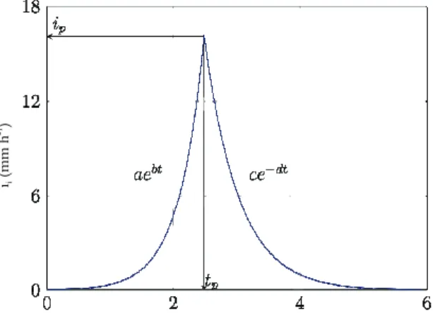
The first change implemented to the original model was the replacement of the rainfall profile based on the IDF (intensity, duration, frequency) curve by a double exponential function (Figure 1). The double exponential profile consists of an increasing exponential from the start of the event up to the time when the maximum rainfall intensity occurs, and a decreasing exponential after this point that describes the behavior of the profile until the end of the event (NICKS et al., 1995). The function is expressed by the equation:
(1)
where:
ii = the instantaneous rainfall intensity (mmh-1);
t = the time from the start of the rainfall (h); tp =
the time to the peak intensity (h); td = the rainfall
duration (h); a, b, c, d = the adjustable parameters (dimensionless).
ii
(mm
h
-1)
Figure 1. Example of a rainfall profile described by a double exponential function, where ii is the instantaneous rainfall intensity, t is the time from the start of the rainfall, ip is the peak intensity, and tp is the time to the peak intensity.
The total rainfall (P, in mm) that occurs during
the considered event, with the duration td, is
obtained by the equation:
(2)
Soil water infiltration
potentially intercepted by the vegetation cover, the rainfall begins to infiltrate the soil. From this
moment, the infiltration rate (f) is equal to the
instantaneous rainfall intensity (ii). This condition is
maintained until the instantaneous rainfall intensity exceeds the soil infiltration capacity and the depressional storage at the soil surface starts. The
cumulative infiltration (F, in mm), which occurs
between the end of the canopy interception and the beginning of the depressional storage, can be estimated by the equation:
(3)
where:
tSL = the duration of the canopy interception
(min.); tiDS = the time when the depressional
storage begins (min.).
From the time the depressional storage begins
(tiDS), the infiltration rate is calculated by the
Green-Amp equation modified by Mein-Larson (GAML):
(4)
where:
f = the infiltration rate (mm h-1); K = the
saturated hydraulic conductivity (mm h-1); θs = the
saturated water content (cm3 cm-3); θi = the initial
water content (cm3 cm-3); ψ
f = the wetting front
suction head (mm); F(t) = the cumulative
infiltration (mm).
This equation for the infiltration rate holds until
the rainfall intensity (ii) becomes equal to the
infiltration rate (f), i.e., until the runoff ends (tfR).
tiDS and tfR are determined using the equation:
(5)
The cumulative infiltration (F, in mm) is
obtained by the sum of the infiltration that occurs during the different phases associated with the water balance and is expressed by the equation:
(6)
where:
tfDS = the time when depressional storage ends (h).
If the rainfall ends before the total depressional storage capacity is filled, infiltration will continue to be expressed by equation 4 until the depressional
storage capacity in the soil is completely filled (tfDS).
In this case, it is necessary to compute the infiltration that occurred after the end of the rainfall in equation 6.
Runoff
The runoff begins when the depressional storage
capacity is filled. The runoff rate (qR, in mm h-1) is
expressed by the equation:
(7)
The total runoff (R, in mm) is obtained by
equation 8. The depressional storage is not considered in this equation because it is added to the infiltration.
(8)
where:
SL = the canopy interception (mm).
Equations 7 and 8, used in the runoff calculation, are the same as those presented by Pruski et al. (2001). However, there are differences in the relationships among the water balance components due the change in the rainfall profile (Figure 2).
Figure 2a presents the components of the water balance in the soil surface using the IDF-based rainfall profile (PRUSKI et al., 2001). The rainfall intensity is at the maximum in the beginning and continually decreases until the end of the event.
Figure 2b presents the components of the water balance at the soil surface using a rainfall profile based on the double exponential equation proposed in this work. The rainfall intensity increases until it reaches its peak and subsequently decreases until the end of event.
In both cases, the water infiltration starts after the canopy interception capacity is completely filled. However, in Figure 2a, the infiltration rate is constantly decreasing, whereas in Figure 2b it increases until the rainfall intensity exceeds the soil infiltration capacity.
intensi
ty
or rat
e
(mm h
-1)
time (h)
intensi
ty
or rat
e
(mm h
-1)
time (h)
Figure 2. Components associated with the water balance in the soil surface proposed by Pruski et al. (2001), with a rainfall profile based on the IDF equation (a), and the water balance proposed in this work, with the rainfall profile based on a double exponential equation (b). IC = the infiltration capacity, SL = the canopy interception, DS = the depressional storage, R = the runoff, F = the infiltration, P = the precipitation.
Model parameterization and evaluation Experimental data
In the model parameterization, the data were obtained from four experimental plots located in the experimental area of the Agriculture and Veterinary Center – CAV of the State University of Santa Catarina (Brazil). The soil in the experiment site is
an Inceptisol consisting of 420 g kg-1 of clay, 170 g
kg-1 of sand and 410 g kg-1 of silt.
The plots were 22.1 m in length (in the direction of the slope) by 3.5 m in width, and the mean slope
is 0.1 m m-1. Each plot was delimited laterally and at
the upper end by galvanized plaques of 2 x 0.2 m that were stuck in the soil up to 10 cm deep. At the lower end, a collecting gutter guided the runoff to a
sedimentation tank with capacity of 750 L. This
tank, is connected to a second tank using a Geib-type divider. With the aid of the divider, only 1/9 of the exceeding volume of the first tank is transferred to the second tank.
The following soil tillage treatments were applied: bare soil with a plowing + disking operation (BS), conventional tillage with a plowing + two disking operation (CT), minimum tillage with chiseling + disking operation (MT), and no-tillage (NT) where the soil did not receive any preparation. The three last treatments were cultivated under the rotation of soya, wheat, vetch, corn, oats and forage turnip. The historical series of rainfall and runoff used in this study covered the period from January 2003 to November 2008.
Rainfall synthetic series
The mean annual rainfall registered in the experimental area, in the period from 2003 to 2008, was 1182 mm, with a standard deviation of 140 mm. The lowest annual rainfall observed was 1027 mm in 2006, and the highest was 1352 mm in 2007.
To represent the rainfall registered in the historical series, the weather generator ClimaBR (ZANETTI et al., 2006) was used. Two synthetic series of rainfall were generated, each with a duration of 6 years.
Initially, a series adjusted on a monthly basis (SAMB) was generated, where the monthly rainfall was adjusted to be equal to the monthly rainfall observed in the historical series.
After composing the SAMB, a daily adjustment was carried out such that both the synthetic and historical series had the same calendar days with rain and the same total rainfall on each day, generating a series adjusted on a daily basis (SADB). In the SADB, it was not possible to adjust the total duration of each rainfall event.
Therefore, the basic difference between the two series is that in the SAMB, the distribution of the rainy days during the month is not required to be equal to the historical series, while in the SADB, both the monthly and the daily rainfall values are identical to those of the historical series.
Management and vegetation cover
The leaf area index (LAI), the random roughness
(RR) and the crop coefficient (Kc) were selected
according to the recommendations found in the literature for cultivations using the rotation system for different soil tillages (ALBERTS et al., 1995; ALLEN et al., 2006).
Soil
Four combinations of methods to determine the
saturated hydraulic conductivity (K) and the wetting
front head pressure (ψf) were investigated.
Combinations 1 and 2 were obtained from Cecílio et al. (2007).
(a)
Combination 1
- The hydraulic conductivity in the saturated
zone (Kw) is equal to the saturated hydraulic
conductivity (K, in mmh-1):
(9)
- The wetting front head pressure (ψf, in mm) is
obtained from the soil porosity and texture, as suggested by Risse et al. (1995):
(10)
here,
(11)
where:
φ = the soil porosity (cm3 cm-3), C = the clay
fraction (kg kg-1), and S = the sand fraction (kg kg-1).
Combination 2
- The saturated hydraulic conductivity (K) is
replaced with the hydraulic conductivity in the
saturation zone (Kw), which is equal to the constant
infiltration rate (fc, in mm h-1), as proposed by Silva
and Kato (1998):
(12)
The wetting front head pressure is obtained using equation 10.
Combination 3
- The saturated hydraulic conductivity (K) is
replaced by the hydraulic conductivity in the
saturation zone (Kw, in mmh-1), which is obtained
as a function of the soil clay fraction (C, in kg kg-1),
as suggested by Alberts et al. (1995):
(13)
- The wetting front head pressure (ψf, in mm) is
obtained from the hydraulic conductivity in the
saturated zone (Kw, in mm h-1), as proposed by
Rawls et al. (1996):
(14)
Combination 4
- The saturated hydraulic conductivity (K) is
replaced by the hydraulic conductivity in the
saturation zone (Kw), which is equal to the
constant infiltration rate (fc), as in equation 12.
- The wetting front head pressure (ψf) is
obtained from equation 14.
The saturated hydraulic conductivity (K) was
defined to be 18 mm h-1, using the data obtained
from Costa et al. (2006). According to the recommendation from Bertol et al. (2001), the
constant infiltration rate (fc) for the no-tillage
treatment in the experimental area is approximately
16.7 mm h-1. For the conventional tillage (CT) and
minimum tillage (MT) treatments, the infiltration
rate was reduced to half of the fc, and for the bare
soil (BS) treatment, the infiltration rate was reduced
to one-third of the fc.
Analysis of the results
The results of the model parameterization were evaluated by comparing the observed and estimated
annual averages using Student’s t-test. To verify if
the model presents overestimation or underestimation tendencies, we analyzed the coefficients of the regression equations between the observed and estimated values (monthly and annual). The adjustment of the equations was
analyzed using the coefficient of determination (r2).
Results and discussion
Model parameterization
Combination 4 (equations 12 and 14) resulted in
the best GAML parameterization. The values of fc
and ψf obtained with this combination are presented
in Table 1.
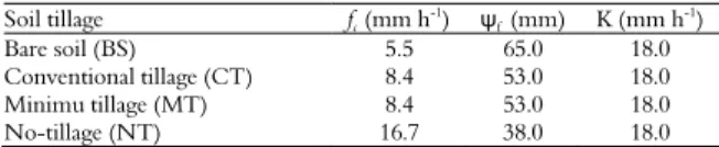
Table 1. Values of the constant infiltration rate (fc), the wetting front head pressure (ψf) and the saturated hydraulic conductivity (K) used for the model evaluation.
Soil tillage fc (mmh-1) ψf (mm) K (mmh-1)
Bare soil (BS) 5.5 65.0 18.0
Conventional tillage (CT) 8.4 53.0 18.0
Minimu tillage (MT) 8.4 53.0 18.0
No-tillage (NT) 16.7 38.0 18.0
Monthly runoff values
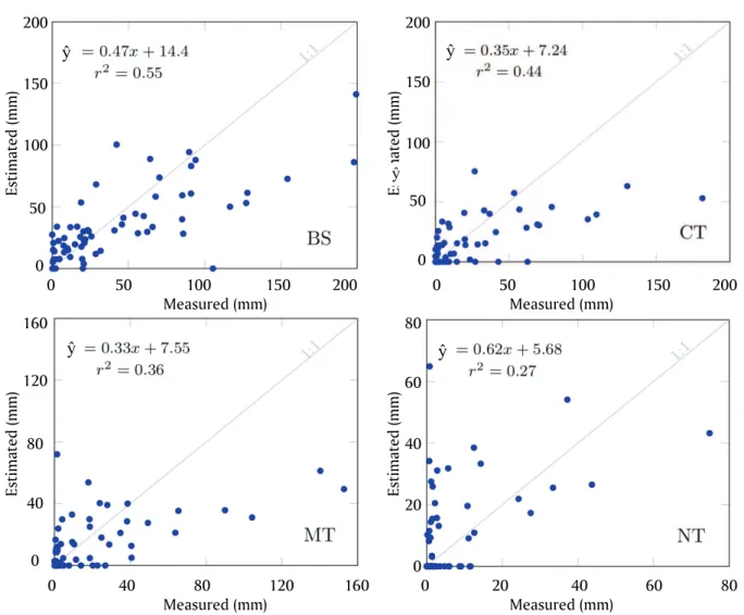
Figure 3 presents the scatter plots for the observed and estimated values of the monthly runoff using the series adjusted on a monthly basis (SAMB). In this figure, the monthly values from the period from 2003 to 2008 were grouped in a single diagram for each type of soil tillage.
the bare soil treatment, (BS, 14.4), and the lowest in the no-tillage treatment (NT, 5.68). The intercepts were similar in the conventional tillage (CT, 7.24) and in the minimum tillage (MT, 7.55) treatments.
The lowest angular coefficients were observed in conventional tillage (CT, 0.35) and minimum tillage (MT, 0.33) treatments, and these values indicate the tendency to underestimate the runoff in the months during which the largest events occur. Although the no-tillage (NT) treatment
was where the lowest r2 occurred (0.27), it was
also where the angular coefficient was closest to 1 and the intercept was closest to zero, among all the treatments.
Figure 4 presents the regression equations for the observed and estimated monthly runoff values using the series adjusted on a daily basis (SADB), in the period from 2003 to 2008. In this figure, the monthly values for all the years were grouped in a single diagram for each type of soil tillage.
In comparison with the SAMB results (Figure 3), it can be observed that the utilization of the SADB (Figure 4) resulted in modifications to the regression coefficients, and increased the coefficients of determination in all types of soil tillage. The intercepts became smaller, and the angular coefficients became closer to 1, indicating an improvement in the estimation of the monthly runoff.
For the bare soil (BS) treatment, the r2 value
increased from 0.55 using the SAMB to 0.66 using the SADB. For the no-tillage (NT) treatment, the increase was from 0.27 to 0.55. The highest increase occurred in the no-tillage (NT) treatment, due to the prevalence of observed values of lower magnitude. With the use of the SADB, there appeared to be an increase in the overestimation of the runoff, causing the slope of the line to increase and the value of the intercept to decrease. This difference may also have favored the lower dispersion of the values around the regression line (Figure 4).
Estimated (m
m)
200
150
100
50
0
Estimated (m
m)
200
150
100
50
0
Measured (mm) Measured (mm)
Estimated (m
m)
160
120
80
40
0
Estimated (m
m)
80
60
40
20
0
0 40 80 120 160 0 20 40 60 80
Measured (mm) Measured (mm)
Figure 3. Regression between the observed and estimated monthly runoff values with the SAMB (series adjusted on a monthly basis) for the bare soil (BS), conventional tillage (CT), minimum tillage (MT) and no-tillage (NT) treatments. The period was from 2003 to 2008. Months with rainfall equal to zero were not considered.
0 50 100 150 200 0 50 100 150 200
ŷ ŷ
ŷ
ŷ
Estimated (m
m)
200
150
100
50
0
Estimated (m
m)
200
150
100
50
0
0 50 100 150 200 0 50 100 150 200
Measured (mm) Measured (mm)
Estimated (m
m)
160
120
80
40
0
Estimated (m
m)
120
90
60
30
0
Measured (mm) Measured (mm)
Figure 4. Regression between the observed and estimated monthly runoff values with the SADB (series adjusted on a daily basis) for the bare soil (BS), conventional tillage (CT), minimum tillage (MT) and no-tillage (NT) treatments. The period was from 2003 to 2008. Months with rainfall equal to zero were not considered.
This increase in the overestimation of the runoff also occurred in the other soil tillages. However, the overestimation of the smallest monthly runoff events was partially compensated for by the underestimation of the largest events.
The differences observed in the regression
coefficients or in the r2 values between the SADB
(Figure 3) and the SAMB (Figure 4) can be explained by the differences between the two synthetic rainfall series.
The two synthetic series had monthly rainfall values equal to those observed in the historical series, but the SAMB (series adjusted on a monthly basis) did not produce the same distribution of rainy days or the same total daily rainfall that was observed in the historical series. However, the SADB (series adjusted on a daily basis) was identical to the historical series, with respect to both the number of rainy days and the total daily rainfall.
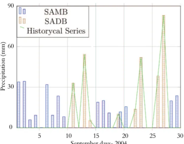
Figure 5 shows the differences between the two synthetic series, and represents the distribution of rainfall observed in the historical series and the distribution obtained with the synthetic rainfall series for September 2004. Only one month was selected at random to simplify the visualization in the graphic.
The rainfall recorded in the experimental area during this month was equal to 289.8 mm. Both the total rainfall obtained with the SAMB and the SADB were equal to the rainfall recorded in the historical series. However, Figure 5 shows that with the use of the SAMB, the rainfall was more evenly distributed along September, with a small predominance of larger events during the first 10 days of the month.
The SADB coincided exactly with the distribution observed in the historical series, presenting a lower number of rainy days, and consequently, higher concentrations of the total precipitation during those days. As shown in Figure 5, five events of large magnitude occurred in September, and they were responsible for 90% of the total monthly rainfall. 0 40 80 120 160 0 30 60 90 120
ŷ ŷ
In the SADB, the rainy days and the total daily rainfall coincided with the historical series; thus, the monthly runoff estimation was better than the estimation performed with the SAMB.
Prec
ip
itat
ion
(m
m
)
90
60
30
0
5 10 15 20 25 30 September days- 2004
Figure 5. Distribution of the daily rainfall for September 2004 and the distribution obtained with the synthetic series SAMB (series adjusted on a monthly basis) and SADB (series adjusted on a daily basis).
Mean annual runoff
Figure 6 presents the mean annual runoff measured and estimated through the model with the utilization of the SAMB and the SADB for the different types of soil tillage.
Mean Annual Runof
f (
mm)
600
500
400
300
200
100
0
BS CT MT NT
Figure 6. Observed and estimated annual runoff with the SAMB (series adjusted on a monthly basis) and the SADB (series adjusted on a daily basis), in bare soil (BS), conventional tillage (CT), minimum tillage (MT) and no-tillage (NT) treatments. Averages of 6 years and confidence intervals (CI) associated with 95% probability are shown.
As expected, the confidence intervals for the means are broad, due to the large standard deviation that typically occurs in works related to water and soil losses. With the exception of the no-tillage treatment, the confidence intervals were higher for the measured averages than the estimated averages.
The mean annual runoff measured was 24, 48 and 35% higher than the mean annual runoff estimated with the SAMB for the bare soil (BS), conventional tillage (CT) and minimum tillage (MT) treatments, respectively, and 22, 41 and 31% higher than the mean annual runoff estimated with the SADB for the same types of soil tillage. In the no-tillage (NT) treatment, the estimated average runoff with SAMB and with SADB was 53 and 67% higher, respectively, than the observed annual average runoff.
However, the deviations presented in Figure 6 were not sufficient to confirm that significant differences existed between the observed and estimated average annual runoff or between the estimated average runoff determined with the use of the SAMB and SADB.
This result confirms the pre-assumption that the use of a synthetic rainfall series for a long simulation period must adequately represent the behavior of the historical series and, consequently, that the average of the results from the synthetic series must be similar to the observed averages. In other words, for long simulation periods, the SAMB may be sufficient to provide an adequate estimation of the annual runoff average.
For short simulation periods, it may be interesting to adopt a synthetic rainfall series in which the distribution of the rainy days and the total daily rainfall are closest to the actual series.
Conclusion
The combination of parameters of the Green-Ampt equation modified by Mein-Larson (GAML) that resulted in the best runoff simulation was
replacing the saturated hydraulic conductivity (K) by
the constant infiltration rate (fc), as suggested by
Silva and Kato (1998), and obtaining the wetting
front head pressure (ψf) from the hydraulic
conductivity of the soil, as suggested by Rawls et al. (1996).
The model overestimated the monthly mean runoff for the months during which the smallest events occurred, and underestimated the monthly mean runoff for the months during which the largest events occurred.
The model underestimated the annual mean runoff for the bare soil (BS), conventional tillage (CT), and minimum tillage (MT) treatments, and overestimated the annual mean runoff for the no-tillage (NT) treatment.
References
ALBERTS, E. E.; NEARING, M. A.; WELTZ, M. A.; RISSE, L. M.; PIERSON, F. B.; ZHANG, X. C.; LAFLEN, J. M.; SIMANTON, J. R. Soil component. In: NSERL. (Ed.). Water erosion prediction project. USDA-ARS. West Lafayette: National Soil Erosion Research Laboratory, 1995. p. 7.1-7.47.
ALLEN, R. G.; PEREIRA, L. S.; RAES, D.; SMITH, M.
Evapotranspiración del cultivo: guías para la determinación de los requerimientos de agua de los cultivos. Roma: Organización de las Naciones Unidas para la Agricultura y la Alimentación, 2006. (Estudio FAO: Riego y Drenaje, 56).
BAIGORRIA, G. A.; ROMERO, C. C. Assesment of erosion hotspots in a watershed: Integrating the WEPP model and GIS in a case study in the Peruvian Andes.
Environmental Modelling and Software, v. 22, n. 8, p. 1175-1183, 2007.
BARRY, D. A.; PARLANGE, J. Y.; LI, L.; JENG, J. S.; CRAPPER, M. Green-Ampt approximations. Advances in Water Resources, v. 28, n. 10, p. 1003-1009, 2005. BERTOL, I.; BEUTLER, J. F.; LEITE, D.; BATISTELA, O. Propriedades físicas de um Cambissolo Húmico afetadas pelo tipo de manejo do solo. Scientia Agricola, v. 58, n. 3, p. 555-560, 2001.
BORMANN, H.; BREUER, L.; GRAFF, T.; HUISMAN, J. A. Analyzing the effects of soil properties changes associated with land use changes on the simulated water balance: a comparison of three hydrological catchment models for scenario analyses. Ecological Modelling, v. 209, n. 1, p. 29-40, 2007.
BOULAIN, N.; CAPPELARE, B.; SÉGUIS, L.; FAVREAU, G.; GIGNOUX, J. Water balance and vegetation change in the Sahel: A case study at the watershed scale with an eco-hydrological model. Journal of Arid Environments, v. 73, n. 12, p. 1125-1135, 2009. CECÍLIO, R. A.; MARTINEZ, M. A.; PRUSKI, F. F.; SILVA, D. D.; ATAÍDE, W. F. Substituição dos parametros do modelo de Green-Ampt-Mein-Larson para estimativa da infiltração em alguns solos do Brasil.
Revista Brasileira de Ciencia do Solo, v. 31, n. 5, p. 1141-1151, 2007.
CHU, X.; MARIÑO, M. Determination of ponding condition and infiltration in layered soils under unsteady rainfall. Journal of Hydrology, v. 313, n. 3-4, p. 195-207, 2005.
COSTA, A.; ALBUQUERQUE, J. A.; ERNANI, P. R.; BAYER, C.; MERTZ, L. M. Alterações físicas e químicas num cambissolo húmico de campo nativo após a correção da acidez. Revista de Ciências Agroveterinárias, v. 5, n. 2, p. 118-130, 2006.
FUJIMAKI, H.; INOUE, M.; KONISHI, K. A multi-step flow method for estimating hydraulic conductivity at low pressure under the wetting process. Geoderma, v. 120, n. 3-4, p. 177-185, 2004.
GÓMEZ, S.; SEVERINO, G.; RANDAZZO, L.; TORALDO, G.; OTERO, J. M. Identification of the
hydraulic conductivity using a global optimization method. Agricultural Water Management, v. 96, n. 3, p. 504-510, 2009.
JI, X. B.; KANG, E. S.; CHEN, R. S.; ZHAO, W. Z.; ZHANG, Z. H.; JIN, B. W. A mathematical model for simulating water balances in cropped sandy soil with flood irrigation applied. Agricultural Water Management, v. 87, n. 3, p. 337-346, 2007.
JIE, Z.; GUANG-YONG, L.; ZHEN-ZHONG, H.; GUO-XIA, M. Hydrological cycle simulation of an irrigation district based on a SWAT model. Mathematical and Computer Modelling, v. 51, n. 11-12, p. 1312-1318, 2010.
LEGESSE, D.; VALLET-COULOMB, C.; GASSE, F. Hydrological response of a catchment to climate and land use changes in Tropical Africa: case study South Central Ethiopia. Journal of Hydrology, v. 275, n. 1-2, p. 67-85, 2003.
MA, Y.; FENG, S.; SU, D.; GAO, G.; HUO, Z. Modelling water infiltration in a large layered soil column with a modified Green-Ampt model and HYDRUS-1D.
Computers and Eletronics in Agriculture, v. 71, n. 1, p. S40-S47, 2010.
MAAYAR, M. E.; PRICE, D. T.; CHEN, J. M. Simulating daily, monthly and annual water balances in a land surface model using alternative root water uptake schemes. Advances in Water Resources, v. 32, n. 9, p. 1444-1459, 2009.
MEIN, R. G.; LARSON, C. L. Modeling infiltration during a steady rain. Water Resources Research, v. 9, n. 4, p. 384-394, 1973.
MELLO, C. R.; VIOLA, M. R.; NORTON, L. D.; SILVA, A. M.; WEIMAR, F. A. Development and application of a simple hydrologic model simulation for a Brazilian headwater basin. Catena, v. 75, n. 3, p. 235-247, 2008.
MOHAMMAD, A. G.; ADAM, M. A. The impact of vegetative cover type on runoff and soil erosion under different land uses. Catena, v. 81, n. 2, p. 97-103, 2010. MOODY, J. A.; KINNER, D. A.; ÚBEDA, X. Linking hydraulic properties of fire-affected soils to infiltration and water repellency. Journal of Hydrology, v. 379, n. 3-4, p. 291-303, 2009.
NICKS, A. D.; LANE, L. J.; GANDER, G. A. Weather generator. In: FLANAGAN, D. C.; NEARING, M. A. (Ed.). Water erosion prediction project (WEPP). West Lafayette: USDA-ARS/National Soil Erosion Research Laboratory, 1995. p. 2.1-2.22.
NOTTER, B.; MCMILLAN, L.; VIRIROLI, D.; WEINGARTNER, R.; LINIGER, H. P. Impacts of environmental change on water resources in the Mt. Kenya region. Journal of Hydrology, v. 343, n. 3-4, p. 266-278, 2007.
RAWLS, W. J.; DAVID, G.; VAN MULLEN, J. A.; WARD, T. J. Infiltration. In: MANAGEMENT GROUP D (Ed.). Hydrology Handbook. New York: ASCE, 1996. p. 75-124. (ASCE Manuals and Report on Engineering Practice, v. 28).
RISSE, L. M.; NEARING, M. A.; ZHANG, X. C. Variability in Green-Ampt effective conductivity under fallow conditions. Journal of Hydrology, v. 169, n. 1-4, p. 1-24, 1995.
SILVA, C. L.; KATO, E. Avaliação de modelos para previsão da infiltração de água em solos sob cerrado. Pesquisa Agropecuária Brasileira, v. 33, n. 7, p. 1149-1158, 1998.
ZANETTI, S. S.; OLIVEIRA, V. P. S.; PRUSKI, F. F. Validação do modelo ClimaBR em relação ao número de dias chuvosos e à precipitação total diária. Engenharia Agrícola, v. 26, n. 1, p. 96-102, 2006.
Received on September 8, 2011. Accepted on December 7, 2011.