Printed version ISSN 0001-3765 / Online version ISSN 1678-2690 http://dx.doi.org/10.1590/0001-3765201720150579
www.scielo.br/aabc
The Extended Log-Logistic Distribution: Properties and Application
STÊNIO R. LIMA and GAUSS M. CORDEIRO Universidade Federal de Pernambuco,
Departamento de Estatística, Av. Prof. Moraes Rego, 1235, Cidade Universitária, 50740-540 Recife, PE, Brazil
Manuscript received on September 3, 2015; accepted for publication on October 7, 2016 ABSTRACT
We propose a new four-parameter lifetime model, called the extended log-logistic distribution, to generalize the two-parameter log-logistic model. The new model is quite flexible to analyze positive data. We provide some mathematical properties including explicit expressions for the ordinary and incomplete moments, probability weighted moments, mean deviations, quantile function and entropy measure. The estimation of the model parameters is performed by maximum likelihood using the BFGS algorithm. The flexibility of the new model is illustrated by means of an application to a real data set. We hope that the new distribution will serve as an alternative model to other useful distributions for modeling positive real data in many areas.
Key words:exponentiated generalize, generating function, log-logistic distribution, maximum likelihood estimation, moment.
INTRODUCTION
Numerous classical distributions have been extensively used over the past decades for modeling data in several areas. In fact, the statistics literature is filled with hundreds of continuous univariate distributions (see, e.g, Johnson et al. 1994, 1995). However, in many applied areas, such as lifetime analysis, finance and insurance, there is a clear need for extended forms of these distributions.
Thelog-logistic(“LL” for short) distribution is a very popular distribution pioneered to model popu-lation growth by Verhulst (1838). In income inequality literature, the LL model is well-known as the Fisk distribution due to Fisk (1961), and has also been widely used in many areas such as reliability, survival analysis, actuarial science, economics, engineering and hydrology. In some cases, the LL distribution is proved to be a good alternative to the log-normal distribution since it characterizes increasing hazard rate function (hrf). Further, its use is well appreciated in case of censored data usually common in reliability and life-testing experiments, Tahir et al. (2014).
The cumulative distribution function (cdf)G(x)and probability density function (pdf)g(x)of the LL
distribution are given by
G(x) =G(x;α,β) = x
β
αβ+xβ, x >0, (1)
and
g(x) =g(x;α,β) = β(x/α)
β−1
α[1 + (x/α)β]2, (2)
respectively, whereα > 0is the scale parameter and also the median of the distribution andβ > 0is the
shape parameter. Some basic properties of the LL distribution are given, for example, by Kleiber and Kotz (2003), Lawless (2003) and Ashkar and Mahdi (2006). The moments (for r < β) are easily derived as,
Tadikamalla (1980)
E(Tr) =αrB(1−rβ−1,1 +rβ−1) = rπα
rβ−1
sin(rπβ−1
), (3)
whereB(a,b) =R01ωa−1(1−ω)b−1
dωis the beta function. Hence,
E(T) = παβ
−1
sin(πβ−1
), β >1 and Var(T) =
2πα2β−1
sin(2πβ−1 ) −
παβ−1
sin(πβ−1 )
2
, β >2.
IfThas a LL distribution with scale parameterαand shape parameterβ, LL(α,β)say, thenW =log(T)
has a logistic distribution with location parameter log(α)and scale parameter1/β. It has attracted a wide
applicability in survival and reliability over the last few decades, particularly for events whose failure rate increases initially and decreases later, for example, mortality from cancer following diagnosis or treatment, Gupta et al. (1999). It has also been used in hydrology to model stream flow and precipitation – see, Shoukri et al. (1988) and Ashkar and Mahdi (2006) – and for modeling flood frequency, see, Ahmad et al. (1988).
For a baseline continuous cdfG(x), Cordeiro et al. (2013) defined theexponentiated generalized(“EG”)
class of distributions by the cdf
F(x) ={1−[1−G(x)]a}b, x∈R, (4)
where a > 0 andb > 0 are two extra parameters whose role is to govern the skewness and generate
distributions with heavier/ligther tails. They are sought as a manner to furnish a more flexible distribution. Because of its tractable cdf (4), this class can be used quite effectively even if the data are censored. The EG class is suitable for modeling continuous univariate data that can be in any interval of the real line. The pdf corresponding to (4) is given by
f(x) =a b [1−G(x)]a−1{1−[1−G(x)]a}b−1g(x), x∈R, (5)
whereg(x) = dG(x)/dxis the baseline pdf. The two parameters in (5) can control both tail weights and
possibly adding entropy to the center of the EG density. The baseline pdfg(x)is a special case of (5) when
a=b= 1. Settinga= 1it gives to the exponentiated-G (“exp-G”) class of distributions. Ifb= 1, we obtain
In this paper, we propose and study some structural properties of a new four-parameter distribution with positive real support, called theextended log-logistic(“ELL”) distribution, derived from equation (5) by takingG(x)andg(x)to be the cdf and pdf of the LL distribution, respectively. We also discuss maximum
likelihood estimation of the model parameters of the proposed distribution. We adopt a different approach to much of the literature so far: rather than considering the beta and Kumaraswamy generators applied to a baseline distribution, we consider the EG generator applied to the LL distribution. The ELL distribution can be applied to positive real data in several areas in a similar manner of the beta log-logistic and Kumaraswamy log-logistic distributions.
The rest of the paper is organized as follows. In Section “The ELL Distribution’, we define the ELL distribution and provide plots of the density and hazard rate functions. In Section “useful representations”, we derive a useful mixture representation for its density function in terms of LL densities. In Section “’Main Properties’, we provide some mathematical properties of the proposed model. In fact, explicit expressions for the ordinary and incomplete moments, a power series expansion for the quantile function (qf), stan-dard measures for the skewness and kurtosis, probability weighted moments, mean deviations and entropy measure. Estimation by the method of maximum likelihood is presented in Section “Maximum Likelihood Estimation”. An application to a real data set illustrates the flexibility of the ELL distribution in Section “Application”. Concluding remarks are given in Section “Conclusions”.
THE ELL DISTRIBUTION
By inserting (1) and (2) in equation (5), we obtain the ELL density function (for x > 0) with positive
parametersa,b,αandβ, say ELL(a,b,α,β), given by
f(x) = abβ(x/α)
β−1
α[1 + (x/α)β]2
1− x
β
αβ+xβ
a−1 1−
1− x
β
αβ+xβ
ab−1
. (6)
The ELL density is straightforward to compute using any statistical software with numerical facili-ties. Also, there is no functional relationship between the parameters and they vary freely in the parameter space. The new distribution due to its flexibility in accommodating non-monotonic hrf may be an impor-tant distribution that can be used in a variety of problems in modeling survival data. The LL and Exp-LL (exponentiated log-logistic) distributions are clearly the most important sub-models of (6) fora = b = 1
anda = 1, respectively. Ifb = 1, we obtain Lehmann type II log-logistic distribution. The cdf and hrf
corresponding to (6) are
F(x) =
1−
1− x
β
αβ+xβ
ab
(7)
and
h(x) =
abβ(x/α)β−1
1− xβ
αβ+xβ
a−1h
1−1− xβ
αβ+xβ
aib−1
α[1 + (x/α)β]2
1−h1−1− xβ
αβ+xβ
aib . (8)
xu =Q(u) =
αβ[1−(1−u1/β)1/α]
(1−u1/β)1/α , u∈(0,1). (9) Quantiles of interest can be obtained from (9) by substituting appropriate values foru. In particular, the
median ofXis
M edian(X) =Q(0.5) = α
β[1−(1−0.51/β)1/α]
(1−0.51/β)1/α .
We can also use (9) for simulating ELL random variables: ifUis a uniform random variable on the unit
interval(0,1), then
X =Q(U) = α
β[1−(1−U1/β)1/α]
(1−U1/β)1/α has the pdf (6).
We consider the generalized binomial expansion
(1−z)b = ∞
X
k=0 (−1)k
b
k
zk, (10)
which holds for any real non-integerband|z|<1. Using (10) in equation (9), we can rewriteQ(u)as
Q(u) = ∞
X
k=1
akuk/β, (11)
where (fork >0)ak = (−1)kαβ 1/kα.
Figures 1 and 2 display some shapes of (6) and (8), respectively, for specified parameter values. The pdf and hrf take various forms depending on the parameter values. The ELL distribution is much more flexible than the LL distribution, that is, the additional shape parameters (aandb) allow for a high degree of its
flexibility. So, the new model can be very useful in many practical situations for modeling positive real data sets.
USEFUL REPRESENTATIONS
Some useful representations for (4) and (5) can be derived using the concept of exponentiated distributions. The properties of these distributions have been studied by many authors in recent years. See, for example, Mudholkar et al. (1995) and Mudholkar and Srivastava (1993) for exponentiated Weibull, Gupta et al. (1998) for exponentiated Pareto, Nadarajah (2005) for exponentiated Gumbel, Nadarajah and Gupta (2007) for exponentiated gamma, and Lemonte (2012) for exponentiated Kumaraswamy (Kw), among others.
Cordeiro and Lemonte (2015) proved, using (10) twice in equation (4), that the EG cdf can be expressed asF(x) =P∞j=0ωj+1Hj+1(x), whereωj+1 =P
∞
m=1(−1)j+m+1
b m
ma
j+1
andHj+1(x)is the exp-G cdf
with power parameterj+ 1. By differentiatingF(x), we can write
f(x) = ∞
X
j=0
0.0 0.5 1.0 1.5
0.0
0.5
1.0
1.5
α =1 β =1.5
x
a=4.5,b=4.5 a=3.5,b=3.5 a=2.5,b=2.5 a=1.5,b=1.5 a=0.5,b=0.5
(a)
0.0 0.5 1.0 1.5 2.0 2.5 3.0
0.0
0.2
0.4
0.6
0.8
1.0
1.2
α =2 β =4
x
a=1.5,b=5 a=2.5,b=3.5 a=3.5,b=2.5 a=4.5,b=1.5 a=6,b=1
(b)
0.0 0.2 0.4 0.6 0.8 1.0
0
1
2
3
4
α =0.5 β =1.5
x
a=1,b=0.1 a=1.3,b=0.2 a=1.5,b=0.3 a=2,b=0.4 a=2.5,b=0.5
(c)
0.0 0.5 1.0 1.5 2.0
0.0
0.5
1.0
1.5
2.0
2.5
α =1 β =3
x
a=0.5,b=0.5 a=1.5,b=1.5 a=2.5,b=2.5 a=3.5,b=3.5 a=5,b=5
(d) Figure 1 -Plots of the ELL pdf for some parameter ponto.
wherehj+1(x)is the exp-G pdf with power parameterj+ 1. Thus, equation (12) reveals that the EG density
function is a mixture of exp-G densities. This result is important to obtain some properties of the EG class from those exp-G properties.
An expansion for (6) can be derived by defining the exponentiated log-logistic (exp-LL) distribution. A random variableZ has the exp-LL distribution with power parameterd >0, sayZ ∼exp-LL(d), if its
cdf and pdf are given, respectively, by
Hd(x) =
xβ
αβ+xβ
d
, hd(x) =
dβ(x/α)β−1
α[1 + (x/α)β]2
xβ
αβ+xβ
d−1
.
First, the expansion holds
(1 +z)−a= ∞
X
n=0
−a
n
zn. (13)
Inserting this expansion inhd(x)gives
hd(x) =
∞
X
n=0
snxβ(d+n)
−1
0.0 0.2 0.4 0.6 0.8 1.0
0
1
2
3
4
5
α =1 β =0.5
x
hazard
a=0.5,b=1.5 a=1.5,b=0.5 a=3.5,b=2.5 a=5,b=3 a=5,b=9
(a)
0.0 0.5 1.0 1.5 2.0
0
1
2
3
4
5
6
α =0.5 β =1
x
hazard
a=1,b=2 a=1.5,b=0.5 a=2.5,b=1.5 a=3.5,b=2.5 a=5,b=9
(b)
0.0 0.5 1.0 1.5 2.0 2.5 3.0
0
1
2
3
4
α =1 β =2
x
hazard
a=1.5,b=0.5 a=1,b=2.5 a=4,b=1.8 a=2,b=5 a=3,b=6
(c)
0.0 0.5 1.0 1.5 2.0 2.5 3.0
0
1
2
3
4
α =1 β =4
x
hazard
a=0.1,b=0.2 a=0.1,b=0.4 a=0.1,b=0.1 a=0.3,b=0.6 a=1.5,b=3
(d) Figure 2 -Plots of the ELL hrf for some parameter ponto.
wheresn= αβdβ(d+n) −d−1
n
. Thus,
hj+1(x) = (j+ 1)β ∞
X
n=0
−j−
2
n
xβ(j+n+1)−1
αβ(j+n+1) . (14)
Inserting the last expression in equation (12) gives
f(x) = ∞
X
j,n=0
ωj+1snxβ(j+n+1)
−1
, (15)
wheresn= α(βj(+1)j+n+1)β −j−2
n .
In a more simplified form, the last equation reduces to
f(x) = ∞
X
j,n=0
whereqj,n=snwj+1. Equation (16) reveals that the ELL density function is a mixture of LL densities. The
cdf corresponding (16) is evidently given by
F(x) = ∞
X
j,n=0
qj,nG(x;α,β(j+n+ 1)). (17)
whereG(x;α,β(j +n+ 1)) denotes the cdf of the LL distribution with shape parameterβ(j+n+ 1).
So, several of the ELL mathematical properties can be obtained form those of the LL distribution. The coefficientsqj,ndepend only on the generator parameters. This equation is the main result of this section.
MAIN PROPERTIES
In this section, we obtain the ordinary and incomplete moments, moment generating function (mgf), qf, probability weighted moments (PWMs), entropy measure and mean deviations of the ELL distribution. The formulas derived throughout the paper can be easily handled in analytical softwares such asMAPLE andMATHEMATICA which have the ability to deal with analytic expressions of formidable size and complexity.
MOMENTS AND GENERATING FUNCTION
We derive a simple expression for therth moment ofX,µ′
r=E(Xr) = R∞
0 x
rf(x)dx. We have
µ′r= ∞
X
j,n=0
qj,n
Z ∞
0
xrg(x;α,β(j+n+ 1))dx.
By using (3), we obtain
µ′r=αrB(1−rβ(j+n+ 1)−1,1 +rβ(j+n+ 1)−1) = rπα
rβ(j+n+ 1)−1
sin(rπβ(j+n+ 1)−1
), (18)
whereB(a,b) =R01ωa(1−ω)b−1
dωis the beta function. Settingr = 1in (18), it follows that the mean of
Xis
µ′1 = παβ(j+n+ 1)
−1
sin(πβ(j+n+ 1)−1).
Further, the central moments(µn)and cumulants(κn)ofXare obtained from (18) as
µs=
p X
k=0
s k
(−1)kµ′1sµ′s−k and κs=µ
′
s− s−1
X
k=1
s−1
k−1
κkµ
′
s−k,
respectively, whereκ1=µ′1. The skewnessγ1 =κ3/κ3/22 and kurtosisγ2=κ4/κ22can be calculated from
the third and fourth standardized cumulants.
Thesth incomplete moment ofXis defined byms(y) = Ry
0 xsf(x)dx. From equation (15), we obtain
ms(y) =
∞
X
j,n=0
qj,n
yβ(j+n+1)+s
β(j+n+ 1) +s. (19)
Applications of these equations to obtain Bonferroni and Lorenz curves are important in several fields such as economics, reliability, demography, insurance and medicine. For a given probability π, these
curves are given by B(π) = m1(q)/πµ′1 and L(π) = m1(q)/µ′1, respectively, where µ ′
1 = E(X),
q = αβ[1(1−−(1u−1/uβ1/)1/β)α1/α]is the qf ofXatπandm1(q)comes from (19) withs= 1.
QUANTILE FUNCTION
The effects of the shape parametersaandbon the skewness and kurtosis can be considered based on quantile
measures. The shortcomings of the classical kurtosis measure are well-known. Bowley skewness, Kenney and Keeping (1962), and Moors kurtosis, Moors (1998), are based on quartiles and octiles given by
B= Q(3/4) +Q(1/4)−2Q(1/2)
Q(3/4)−Q(1/4)
and
M= Q(3/8)−Q(1/8) +Q(7/8)−Q(5/8)
Q(6/8)−Q(2/8) ,
respectively. Clearly,M>0and there is good concordance with the classical kurtosis measures for some
distributions. These measures are less sensitive to outliers and they exist even for distributions without moments.
Now, consider an equation for a power series raised to a positive integerr
∞
X
m=0
wmxm
!r
= ∞
X
m=0
pr,mxm, (20)
given in Gradshteyn and Ryzhik (2007), where the coefficientspr,m (form = 1,2, . . .) can be determined fromw0, . . . ,wmbased on the recurrence equationpr,m = (m w0)−1Pmk=1[(r+ 1)k−m]wkpr,m−k, with
pr,0 =wr0. Clearly,pr,mcan be computed numerically in any algebraic or numerical software. Using (10) in equation (9), we can rewriteQ(u)as
Q(u) = ∞
X
j=1
sjuj/β, u∈(0,1), (21)
wheresj =αβ(−1)j
−1/α
j
.
LetW(·)be any integrable function in the positive real time. We can write
Z ∞
0
W(x)f(x)dx=
Z 1
0
W
∞
X
j=1
sjuj/β
du. (22)
Equations (21) and (22) are the main results of this section since various ELL mathematical quan-tities can follow from them. For example, µ′n = R01(P∞j=1sjuj/β)ndu = P
∞
j=1 hn,j R1
0 uj/bdu =
P∞
PROBABILITY WEIGHTED MOMENTS
The PWMs of a random variableT with cdfG(X)are defined byδs,r =E[XsG(X)r]forsandrpositive integers. Here, the PWMs of the LL distribution are used to compute the ordinary moments of the ELL distribution. IfT ∼LL(α,β), fors < β, we obtain
δs,r =
β αβ
Z ∞
0
xs+β−1
1 +x
α
β−2(
1−
1 +x
α
β−1)r
dx
= αs
Z 1
0
ω−sβ−1
(1−ω)r+sβ−1
dω=αsB(r+ 1 +sβ−1,1−sβ−1). (23)
The ordinary moments ofXfollow asδs,0 =E(Xs). Based on (21), we can write
δs,r = Z 1
0
∞
X
j=1
sjuj/β s
urdu.
Then, using (20), we obtain
δs,r =
∞
X
j=1
ts,j Z 1
0
ur+j/bdu= ∞
X
j=1
ts,j
r+j/b+ 1, (24)
wherets,j = (j ν0)−1Pjk=1[(s+ 1)k−j]νkhs,j−k andts,0 = ν0s. Equation (24) is very simple to be
calculated analytically or numerically using symbolic computer systems.
MEAN DEVIATIONS
The amount of scatter in a population is evidently measured to some extent by the totality of deviations from the mean and median. The mean deviations about the mean (δ1 =E(|X−µ′1|)) and about the median
(δ2 =E(|X−M|)) ofXcan be expressed asδ1 = 2µ′1F(µ ′
1)−2m1 (µ′1)andδ2(X) =µ ′
1−2m1(M),
respectively, whereµ′1 = E(X), M = M edian(X) is the median, and m1(z) is the first incomplete
moment obtained from (19) withs= 1.
ENTROPY MEASURE
Entropy has been used in various situations in science as a measure of variation of the uncertainty. Numerous measures of entropy have been studied and compared in the literature. LetX ∼ ELL(a,b,α,β). Here, we
shall derive an explicit expression for the Shannon entropy. We consider this entropy since it plays a similar role as the kurtosis measure in comparing the shapes of various densities and measuring heaviness of the tails. It is defined byIS =E{−log[f(X)]}, which implies
IS =−log
abβ α
−(a−1)Ehlogαβα+βxβ
i
−(b−1)Enlogh1− αβ
αβ+xβ
io
−(β−1)Elog αx+ 2Elog1 + x
α .
E
h logx
α
i
= ba
bαβ(a+2b−ab−1)
βΓ(ab+ 1) Γ(b)Γ(b(a−1) + 1)×
n
βlog(1/α)−log(α−β) +ψ(b)−ψ[b(a−1) + 1]o
− (b−1)α
βa(1−b)
[γ−1 +βlog(1/α) +log(α−β) +ψ(ab−1)]
β(ab−1)
+ abα
β(ab−2)+1
βΓ(ab+ 1) Γ(a−1/β+ 2)Γ(a(b−1) + 1/β−1)×
n
βlog(1/α)−log(αβ)−ψ(a−1/β+ 2) +ψ(a(b−1) + 1/β−1)o.
Some other expected values can be determined analytically using theMATHEMATICAsoftware and they can be obtained from the authors upon request.
MAXIMUM LIKELIHOOD ESTIMATION
We consider the estimation of the unknown parameters of the ELL distribution by the method of maxi-mum likelihood. Letx1, . . . , xnbe a random sample from (6). LetΘ = (a,b,α,β)⊤be the vector of model parameters. The log-likelihood function logL=logL(θ)forθis given by
logL =nlogabβα + (a−1)Pni=1logαβα+βxβ i
+ (b−1)Pni=1logh1− αβ
αβ+xβ i
ai
+(β−1)Pni=0log x α
−2Pni=0logh1 + x
α βi
. (25)
Maximization of (25) can be performed by using well-established routines like NLM or OPTIMIZE in the R statistical package, NLMIXED procedure in the SAS or MaxBFGS in the Ox program or, alternatively, by solving the nonlinear likelihood equations obtained by differentiating (25).
The components of the score vectorU =U(θ) = (∂logL/∂a, ∂logL/∂b, ∂logL/∂α, ∂logL/∂β)⊤
are given by
∂logL
∂a =
n
a +nlog(α
β)−nlog(αβ+xβ)− n X
i=0
a(b−1) α
βa(αβ+xβ)
α[a(αx)β+xβa]
,
∂logL
∂b = n b + n X i=0
log1−
αβ
αβ +xβ
a
,
∂logL
∂α = −
n
α −
n(β−1)
α + (a−1)
n X
i=0
βαβ−1
xβ
αβ(αβ+xβ)+ n X
i=0
a(b−1)βαβa−1
xβ
a(αx)β +xβa +
2
n X
i=0
αββxβ αβ(αβ+xβ),
∂logL
∂β =
n
β + (a−1)
n X
i=0
(αx)βlog(αx)
(αβ+xβ)2 +
n X
i=0
a(b−1)αβaxβlog(α/x)
a(αx)β+xβa +
n X
i=0
logx
α − 2 n X i=0
αβxβ−1
The maximum likelihood estimates (MLEs) in(θ), say( ˆθ), are the simultaneous solutions of the
equa-tions∂L/∂θ =0. For interval estimation and tests of hypotheses on the model parameters, we require the 4×4observed information matrixJ(θ), whose elements can be obtained from the authors under request.
Upon conditions that are fulfilled for parameters in the interior of the parameter space, the asymptotic distribution of(θb−θ)isN4(0,J(θ)−1
), which can be used to construct approximate confidence intervals
and confidence regions for the parameters. We believe that the standard likelihood regularity conditions are satisfied for the ELL model. These conditions are: i) the support of the distribution does not depend on unknown parameters; ii) the parameter space is open and the log-likelihood function has a global maxi-mum in it; iii) the third order log likelihood derivatives have finite expected values; iv) the fourth order log likelihood derivatives exist almost everywhere, and are continuous in an open neighborhood that contains the true parameter value; v) the expected information matrix is positive definite and finite. These regularity conditions hold for almost distributions which satisfy i). So, they are not restrictive.
APPLICATION
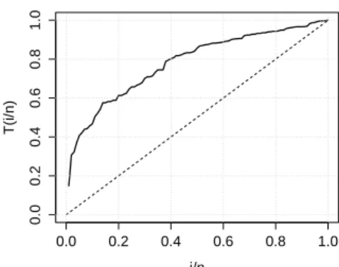
In this section, we compare the fits of the ELL distribution defined in (6), the exponentiated log-logistic (ELLog) Rosaiah et al. (2006), McDonald log-logistic (McLL) Tahir et al. (2014), beta log-logistic (BeLL) Lemonte (2012), Kumaraswamy log-logistic (KwLL) de Santana et al. (2012), Marshal-Olkin log-logistica (MoLL) Gui (2013) and log-logistic (LL) to a real data set. In many applications there is qualitative information about the hrf, which can help with selecting a particular model. In this context, a device called the total time on test (TTT) plot Aarset (1987) is useful. The TTT plot is obtained by plotting
G(r/n) = [(Pri=1yi:n) + (n−r)yr:n]/Pni=1yi:n, wherer = 1, . . . , nandyi:n (i = 1, . . . , n) are the order statistics of the sample, againstr/n. It is a straight diagonal for constant failure rates, it is convex for
decreasing failure rates and concave for increasing failure rates. It is first convex and then concave if the failure rate is bathtub-shaped. It is first concave and then convex if the failure rate is upside-down bathtub. We consider an uncensored data set from Nichols and Padgett (2006) consisting of 100 observations on breaking stress of carbon fibres (in Gba). TheTTTplot for the exceedances of flood peaks data in Figure 3 indicates a bathtub-shaped hrf and, therefore, the appropriateness of the ELL distribution to fit these data.
0.0 0.2 0.4 0.6 0.8 1.0
0.0
0.2
0.4
0.6
0.8
1.0
i/n
T(i/n)
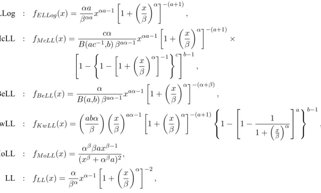
Further, we fit the ELL, ELLog, McLL, BeLL, KwLL, MoLL and LL models (for x > 0) with
corresponding densities:
ELLog : fELLog(x) =
αa βαax
αa−1
1 +
x
β
α−(a+1)
,
McLL : fM cLL(x) =
cα B(ac−1
,b)βaα−1x
αa−1
1 +
x
β
α−(a+1)
× " 1− ( 1− 1 + x β
α−1)c#b−1
,
BeLL : fBeLL(x) =
α
B(a,b)βaα−1x
aα−1
1 +
x β
α−(α+β)
,
KwLL : fKwLL(x) =
abα β
x β
aα−1 1 +
x β
α−(a+1)
1−
1− 1
1 +xβα
a
b−1
,
MoLL : fM oLL(x) =
αββaxβ−1
(xβ+αβa)2,
LL : fLL(x) =
α βαx
α−1
1 +
x β
α−2
,
wherea, b, c >0,α >0andβ >0.
Table I lists the MLEs of the parameters (their standard errors are given in parentheses) for the ELL, ELLog, McLL, BeLL, KwLL, MoLL and LL models fitted to the exceedances of flood peak data. We es-timate the unknown parameters of each model by maximum likelihood. There exists many maximization methods in R packages like NR (Newton-Raphson), BFGS (Broyden-FletcherGoldfarb-Shanno), BHHH (Berndt-Hall-Hall-Hausman), SANN (Simulated-Annealing) and NM (Nelder-Mead). The MLEs are cal-culated using the Limited Memory quasi-Newton code for Bound-constrained optimization (L-BFGS-B). Further, the Anderson-Darling(A∗
)and Cramér-Von Mises(W∗
)statistics are computed to compare the
fitted models. The computations are carried out using the R-packageAdequacyModelgiven freely from http://cran.r-project.org/web/packages/AdequacyModel/AdequacyModel.pdf.
Plots of the estimated pdfs and cdfs of the fitted models are displayed in Figure 4. It is clear that the ELL, BeLL and McLL distributions present practically the same fits, i.e., there is significant difference among the curves. Additionally, these plots indicate that these models provide better fits than the other models.
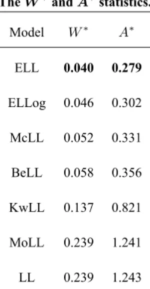
The statisticsW∗ andA∗ are described in Chen and Balakrishnan (1995). In general, the smaller the
values of these measures, the better the fit to the data. The statisticsW∗and
A∗ for all models fitted to the
TABLE I
The MLEs (standard errors in parentheses) of the model parameters.
Model Estimates AIC
ELL(a,b,α,β) 3.607 4.989 1.885 0.548 288.80
(0.176) (0.751) (0.137) (0.032)
ELLog(a,α,β) 3.369 7.345 0.336 288.92
( 0.219) (1.494) (0.098)
McLL(a,b,c,α,β) 0.506 1.996 1.214 4.985 3.729 292.34
(0.162) (0.429) (3.439) (33.868) (0.966)
BeLL(a,b,α,β) 3.424 4.891 0.851 5.359 290.38
(39.488) (0.171) (0.148) (0.381)
KwLL(a,b,α,β) 2.448 10.821 0.014 0.172 296.81
(0.026) (0.055) (0.001) (0.012)
MoLL(a,α,β) 1.800 4.125 3.843 298.55
(30.412) (0.344) (267.146)
LL(α,β) 2.499 4.109 296.55
(0.105) (0.343)
x
0 1 2 3 4 5 6
0.0
0.1
0.2
0.3
0.4
ELL ELLog MoLL BeLL KwLL McLL LL
(a)
1 2 3 4 5
0.0
0.2
0.4
0.6
0.8
1.0
cdf
x
cdf
ELL ELLog MoLL BeLL KwLL McLL LL
(b)
TABLE II TheW∗andA∗statistics.
Model W∗ A∗
ELL 0.040 0.279 ELLog 0.046 0.302 McLL 0.052 0.331 BeLL 0.058 0.356 KwLL 0.137 0.821 MoLL 0.239 1.241 LL 0.239 1.243
CONCLUSIONS
In this paper, we propose a new four-parameter distribution, called the extended log-logistic (ELL) distri-bution, and study some of its general structural properties. This distribution has the support in the positive real interval. Further, the new distribution includes as special models other known distributions. We pro-vide explicit expressions for the ordinary and incomplete moments, probability weighted moments, quantile function, mean deviations and entropy measure. The model parameters are estimated by maximum likeli-hood. The usefulness of the new model is illustrated by means of one application to real data. For these data the new model provides a consistently better fit than other known lifetime models. We hope that the proposed model may attract wider applications for modeling positive real data sets in many areas such as engineering, survival analysis, hydrology, economics, among others.
REFERENCES
AARSET MV. 1987. How to identify bathtub hazard rate. IEEE T Rehabil Eng 36: 106-108.
AHMAD MI, SINCLAIR CD AND WERRITTY A. 1988. Log-logistic ood frequency analysis. J Hydrol 98: 205-224. ASHKAR F AND MAHDI S. 2006. Fitting the log-logistic distribution by generalized moments. J Hydrol 328: 694-703. CHEN G AND BALAKRISHNAN N. 1995. A general purpose approximate goodness-of-fit test. J Qual Technol 27: 154-161. CORDEIRO GM, LEMONTE AL AND CAMPELO AK. 2016. Extended Arcsine Distribution to Proportional Data: Properties
and Applications. Stud Sci Math Hung 53.
CORDEIRO GM, ORTEGAM EMM AND DA CUNHA DCC. 2013. The exponentiated generalized class of distributions. JDS 11: 1-27
DE SANTANA TVF, ORTEGA EMM, CORDEIRO GM AND SILVA GO. 2012. The Kumaraswamy-log-logistic distribution. J Stat Theor Appl 11: 265-291.
FISK PR. 1961. The graduation of income distribution. Econometrica 29: 171-185.
GRADSHTEYN IS AND RYZHIK IM. 2007. Table of Integrals, Series, and Products. Academic Press, New York.
GUI W. 2013. Marshall-Olkin extended log-logistic distribution and its application in minification processes. Appl Math Sci 7: 3947-3961.
GUPTA RC, GUPTA PL AND GUPTA RD. 1998. Modeling failure time data by Lehman alternatives. Commun Stat Theor Meth 27: 887-904.
JOHNSON N, KOTZ S AND BALAKRISHNAN N. 1994. Continuous Univariate Distributions -Volume 1, 2nded., New York: J
Wiley, p. 284-285.
KENNEY JF AND KEEPING ES. 1962. Mathematics of Statistics, Part 1, 3rded., Princeton, NJ, p. 101-102.
KLEIBER C AND KOTZ S. 2003. Statistical Size Distributions in Economics and Actuarial Sciences. J Wiley: New York. LAWLESS JF. 2003. Statistical Models and Methods for Lifetime Data. J Wiley: New York.
LEMOENTE AL. 2015. The beta log-logistic distribution. Braz J Probab Stat 29: 172-173. MOORS JJA. 1998. A quantile alternative for kurtosis. J Roy Stat Soc D 37: 25-32.
MUDHOLKAR GS AND SRIVASTAVA DK. 1993. Exponentiated Weibull family for analyzing bathtub failure-rate data. IEEE T Rehabil Eng 42: 299-302.
MUDHOLKAR GS, SRIVASTAVA DK AND FREIMER M. 1995. The exponentiated Weibull family: A reanalysis of the bus-motor-failure data. Technometrics 37: 436-445.
NADARAJAH S. 2005. The exponentiated Gumbel distribution with climate application. Environmetrics 17: 13-23.
NADARAJAH S AND GUPTA AK. 2007. The exponentiated gamma distribution with application to drought data. Calcutta Statist Assoc 59: 29-54.
NICHOLS MD AND PADGETT WJ. 2006. A Bootstrap control chart for Weibull percentiles. Qual Reliab Eng Int 22: 141-151. ROSAIAH K, KANTAM RRL AND KUMAR CHS. 2006. Reliability test plans for exponentiated log-logistic distribution. Econ
Qual Control 21: 279-289.
SHOUKRI MM, MIAN IUH AND TRACY DS. 1988. Sampling properties of estimators of the log-logistic distribution with application to canadian precipitation data. Can J Stat 16: 223-236.
TADIKAMALLA PR. 1980. A look at the Burr and related distributions. Int Stat Rev 48: 337-344.
TAHIR MH, MANSOOR M, ZUBAIR M AND HAMEDANI GG. 2014. McDonald Log-Logistic distribution. J Stat Theory Appl 13: 65-82.