The Lindley Weibull Distribution: properties and applications

Printed version ISSN 0001-3765 / Online version ISSN 1678-2690 http://dx.doi.org/10.1590/0001-3765201820170635

www.scielo.br/aabc | www.fb.com/aabcjournal

The Lindley Weibull Distribution: properties and applications

GAUSS M. CORDEIRO1_{, AHMED Z. AFIFY}2_{, HAITHAM M. YOUSOF}2_, SELEN CAKMAKYAPAN3_{and GAMZE OZEL}4

1_{Departamento de Estatística, Universidade Federal de Pernambuco, Cidade Universitária,} Avenida Prof. Moraes Rego, 1235, 50740-540 Recife, PE, Brazil

2_{Department of Statistics, Mathematics and Insurance, Benha University, Benha, 13518 Egypt} 3_{Department of Statistics, Istanbul Medeniyet University, 34700 Istanbul, Turkey}

4_{Department of Statistics, Hacettepe University, 68000 Ankara, Turkey}

Manuscript received on August 15, 2017; accepted for publication on November 16, 2017

ABSTRACT

We introduce a new three-parameter lifetime model called the Lindley Weibull distribution, which accom-modates unimodal and bathtub, and a broad variety of monotone failure rates. We provide a comprehensive account of some of its mathematical properties including ordinary and incomplete moments, quantile and generating functions and order statistics. The new density function can be expressed as a linear combination of exponentiated Weibull densities. The maximum likelihood method is used to estimate the model param-eters. We present simulation results to assess the performance of the maximum likelihood estimation. We prove empirically the importance and flexibility of the new distribution in modeling two data sets.

Key words:Lindley G-Family, maximum likelihood, moments, order statistics.

1 - INTRODUCTION

We propose a new generalization of the Weibull (W) distribution named the Lindley Weibull (LiW) model. The W distribution has been widely used in reliability analysis and in applications of several different fields; see, for example Lai et al. (2003). Although its common use, a negative point of the distribution is the limited shape of its hazard rate function (hrf) that can only be monotonically increasing or decreasing or constant.

Generally, practical problems require a wider range of possibilities in the medium risk, for example, when the lifetime data present a bathtub shaped hazard function such as human mortality and machine life cycles. Researchers in the last years developed various extensions and modified forms of the W distribution to obtain more flexible distributions. A state-of-the-art survey on the class of such distributions can be found in Lai et al. (2001) and Nadarajah (2009).

Some extensions of the W distribution are available in the literature such as the exponentiated W (exp-W) (Mudholkar et al. 1993, 1995, 1996), additive W (Xie and Lai 1995), Marshall–Olkin extended W

tany et al. 2005), modified W (Lai et al. 2003, Sarhan and Zaindin 2009), extended W (Xie et al. 2002), beta-W (Lee et al. 2007), beta modified W (Silva et al. 2010), Kumaraswamy W (Cordeiro et al. 2010), transmuted W (Aryal and Tsokos 2011), Kumaraswamy inverse W (Shahbaz et al. 2012), exponentiated generalized W (Cordeiro et al. 2013), McDonald modified W (Merovci and Elbatal 2013), beta inverse W (Hanook et al. 2013), transmuted additive W (Elbatal and Aryal 2013), McDonald W (Cordeiro et al. 2014a), Kumaraswamy modified W (Cordeiro et al. 2014b), transmuted complementary W geometric (Afify et al. 2014), transmuted exponentiated generalized W (Yousof et al. 2015), Marshall–Olkin additive W (Afify et al. 2018, Kumaraswamy transmuted exponentiated additive W (Nofal et al. 2016), generalized transmuted W (Nofal et al. 2017), Topp-Leone generated W (Aryal et al. 2017) and Kumaraswamy complementary W geometric (Afify et al. 2017) distributions. Among these models, the exp-W is certainly the most popular one.

Recently, Cakmakyapan and Ozel (2017) proposed a new class of distributions called the Lindley gener-ator (Li-G) with one extra parameter. For an arbitrary baseline cumulative distribution function (cdf)G(x;ξ),

the Li-G family with one extra positive shape parameterθ has cdf and probability density function (pdf)

(forx>0) given by

F(x;θ,ξ) =1−[1−G(x;ξ)]θ

1− θ

θ+1logG(x;ξ)

(1)

and

f(x;θ,ξ) = θ

2

θ+1g(x;ξ) [1−G(x;ξ)]

θ−1

1−logG(x;ξ), (2)

respectively, whereg(x;ξ) =dG(x;ξ)/dx,G(x;ξ) =1−G(x;ξ)andθ is a positive shape parameter.

The cdf and pdf of the W distribution are given by

G(x;α,β) =1−exp[−(αx)β] (3)

and

g(x;α,β) =β αβxβ−1exp[−(αx)β], (4)

respectively, whereα>0is a scale parameter andβ >0is a shape parameter.

The main objectives of this paper is to obtain a more flexible model by inducting just one extra shape parameter to the W model and to improve goodness-of-fit to real data. The basic motivations for the LiW distribution in practice are: (i) to make the kurtosis more flexible as compared to the baseline model; (ii) to produce skewness for symmetrical distributions; (iii) to construct heavy-tailed distributions that are not longer-tailed for modeling real data; (iv) to generate distributions with symmetric, left-skewed, right-skewed and reversed-J shaped; (v) to provide consistently better fits than other generated models under the same underlying distribution.

takes values from 0.75 to 10. Further, the spread for the LiW kurtosis is much larger ranging from 2.7 to 82, whereas the spread for the W kurtosis only varies from 2.85 to 18.98 with the above parameter values.

Based on the Li-G family, we construct the LiW distribution and provide a comprehensive descrip-tion of some of its mathematical properties. The paper is outlined as follows. In Secdescrip-tion 2, we define the LiW distribution. In Section 3, we derive useful representations for the pdf and cdf of the new distribution. Some mathematical properties including the ordinary and incomplete moments and other types of moments, quantile function (qf), moment generating function (mgf), order statistics and quantile spread order are in-vestigated in Section 4. In Section 5, we obtain the maximum likelihood estimates (MLEs) of the model parameters. In Section 6, we verify the consistency of the estimates by means of some simulations. In Sec-tion 7, we prove empirically that the LiW distribuSec-tion provides better fits than other seven lifetime models, each one having the same number of parameters, by means of two applications to real data sets. Finally, in Section 8, we provide some concluding remarks.

2 - THE LIW DISTRIBUTION

In this section, we define the LiW model and provide some plots of its pdf and hrf. The LiW cdf is given by

F(x) =F(x;θ,α,β) =1−exph−θ(αx)βi1+ θ

θ+1(αx)

β_{. (5)}

The pdf corresponding to (5) is given by

f(x) = f(x;θ,α,β) = β θ

2

θ+1

h

αβxβ−1+α2β_x2β−1i_exph_−θ(αx)βi

. (6)

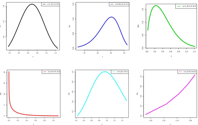
The LiW model is very attractive to define special models with different types of hazard rates. Figure 1 displays some plots of the LiW density for different values ofα, β andθ. These plots reveal that the

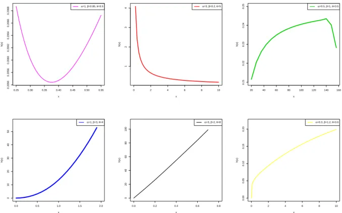
LiW density can be symmetric, left-skewed, right-skewed or reversed J-shape. The hrf plots of the LiW distribution given in Figure 2 can be bathtub, unimodal, reversed J-shape, increasing and decreasing shapes.

3 - LINEAR REPRESENTATION

In this section, we obtain a very useful linear representation for the LiW density. An expansion for (6) can be derived using the very popular exponentiated Weibull (exp-W) distribution, whose applications have been widespread in several areas. A random variableZhas the exp-W density with the baseline W given in (3)

and power parameterd>0, sayZ∼exp-W(d), if its cdf and pdf (forz>0) are given by

Hd(z) =

n

1−exph−(αz)βiod,

and

hd(z) =dβ αβzβ−1exp

h

−(αz)βin1−exph−(αz)βiod−1, respectively.

Using the generalized binomial expansion, the Li-G cdf in (1) can be expressed as

F(x) =1−

∞

∑

k=0

(−1)k

θ k

G(x)k+ θ

θ+1logG(x)

∞

∑

k=0

(−1)k

θ k

0.2 0.4 0.6 0.8 1.0 1.2 0.5 1.0 1.5 x f(x)

α=1, β=3, θ=2.84

25 30 35 40

0.00 0.05 0.10 0.15 x f(x)

α=0.025, β=10, θ=4

0.0 0.2 0.4 0.6 0.8 1.0 1.2

0.0 0.5 1.0 1.5 x f(x)

α=1, β=1.5, θ=4

0.0 0.2 0.4 0.6 0.8 1.0

0 5 10 15 20 x f(x)

α=2, β=0.75, θ=3

0.2 0.4 0.6 0.8 1.0 1.2 1.4

0.2 0.4 0.6 0.8 1.0 x f(x)

α=4, β=2, θ=0.1

1.20 1.22 1.24 1.26

0.2 0.4 0.6 0.8 1.0 x f(x)

α=1, β=15, θ=0.01

Figure 1 -Plots of the LiW pdf for selected parameter values.

Consider the logarithmic power series given by

log(1−b) =− ∞

∑

j=1

bj+1

j+1, |b|<1.

We can write

logG(x) =− ∞

∑

j=1

G(x)j+1

j+1

and then equation (7) becomes

F(x) =1+

∞

∑

k=0

(−1)k+1

_θ

k

G(x)k+ θ

θ+1

∞

∑

k,j=0

(−1)k+1

j+1

_θ

k

G(x)k+j+1.

Equivalently, we obtain

F(x) =1+

∞

∑

k=0

wkHk(x) +

∞

∑

k,j=0

wk,jHk+j+1(x),

wherewk= (−1)k+1 θ_k

andwk,j= θ(−1)

k+1

(j+1)(θ+1)

θ k

.

By differentiating the last equation, the LiW pdf reduces to

f(x) =

∞

∑

k=0

wk+1hk+1(x) +

∞

∑

k,j=0

0.25 0.30 0.35 0.40 0.45 0.50 0.55

0.2056

0.2058

0.2060

0.2062

0.2064

0.2066

0.2068

x

h(x)

α=1, β=0.85, θ=0.5

0 2 4 6 8 10

1

2

3

4

x

h(x)

α=3, β=0.2, θ=5

20 40 60 80 100 120 140 160

0.21

0.22

0.23

0.24

0.25

x

h(x)

α=0.5, β=1, θ=0.5

0.0 0.5 1.0 1.5 2.0

0

10

20

30

40

50

x

h(x)

α=1, β=3, θ=4

0.0 0.2 0.4 0.6 0.8

0

20

40

60

80

100

x

h(x)

α=3, β=2, θ=8

0 2 4 6 8 10

0.00

0.05

0.10

0.15

0.20

x

h(x)

α=0.3, β=1.2, θ=0.6

Figure 2 -Plots of the LiW hrf for selected parameter values.

wherehd(x)denotes the exp-W density with power parametersd. Equation (8) reveals that the LiW density

can be expressed as a linear combination of exp-W densities. Thus, several mathematical properties of the new model can be obtained from those properties of the exp-W distribution. This is the main result of this section. The hrf of the exp-W model allows for constant, monotonically increasing, monotonically decreas-ing, unimodal and bathtub shaped hazard rates. So, these forms also hold for the hrf of the new distribution (as shown in Figure 2).

4 - SOME PROPERTIES

The formulas derived in this section are simple and manageable, and with the use of modern computer resources and their numerical capabilities, the LiW model may prove to be a useful addition to those distributions applied for modeling data in economics, medicine, reliability, engineering, among other areas.

4.1 - ORDINARY AND INCOMPLETE MOMENTS

First, we provide explicit formulas for therth ordinary and incomplete moments of the exp-G random

variableZ(defined in the last section) given by

E(Zr) =dα−rΓ

1+ r

β

∞

∑

i=0

b(_id)

and

mr,Z(y) =

Z y

0

zrhd(z)dz=dα−rγ

1+ r

β,(αz)

β ∞

∑

i=0

b(_id),

respectively, whereb(_id)= (−1)i(i+1)−r/β−1 d−_i1,Γ(p) =R₀∞xp−1e−xdxis the complete gamma function

andγ(p,z) =R₀zxp−1e−xdxis the lower incomplete gamma function.

Second, thesth ordinary moment ofX, sayµ_s′, follows from (8) and the above results as

µ_s′=K1

" _∞

∑

k,i=0

(k+1) wk+1b(ik+1)+ ∞

∑

k,j,i=0

(k+j+1) wk,jb

(k+j+1)

i

# ,

whereK1=α−sΓ

1+ s β

.

The mean, variance, skewness and kurtosis of the LiW distribution are computed numerically forα=1

and some selected values ofβandθusing the R software. The numerical values displayed in Table I indicate

that the skewness of the new distribution can range in the interval(−0.9, 6.5). The spread for its kurtosis

is much larger ranging from2.7to82.

Third, thesth incomplete moment ofX, sayϕs(z) =

Rz

0xsf(x)dx, can be expressed from (8) as

ϕs(z) =K2(z)

" _∞

∑

k,i=0

(k+1)wk+1b(ik+1)+ ∞

∑

k,j,i=0

(k+j+1)wk,jb

(k+j+1)

i

#

, (9)

whereK2(z) =α−sγ

1+ s β,(αz)

β_.

The first incomplete momentϕ1(t)given by (9) (withs=1) has some important applications. For ex-ample, the mean deviations about the mean[θ1=E(|X−µ₁′|)]and about the median[θ2=E(|X−M|)] of X are given by θ1 =2µ

′

1F(µ1′)−2ϕ1(µ1′) and θ2 = µ1′ −2ϕ1(M), respectively, where µ1′ =E(X),

M=Median(X) =Q(0.5)is the median (see Section 4.2) andF(µ′

1)is easily calculated from (5).

The Bonferroni and Lorenz curves are defined (for a given probabilityπ) byB(π) =ϕ1(q)/(π µ1′)and

L(π) =ϕ1(q)/µ1′, respectively, whereq=Q(π)is the qf ofX atπ.

Fourth, thenth moment of the residual life ofX, saymn(z) =E[(X−z)n|X>z],n=1,2,… andz>0,

uniquely determinesF(x), and it is given by

mn(z) = 1

1−F(z)

Z ∞

z

(x−z)ndF(x).

Using equation (8), we can write

mn(z) =

1 1−F(z)

n

∑

r=0

(−1)n−r_(n+1) r zn−r

r! K2(z)

×

" _∞

∑

k,i=0

(k+1) wk+1b(ik+1)+ ∞

∑

k,j,i=0

(k+j+1) wk,jb

(k+j+1)

i

TABLE I

Mean, variance, skewness and kurtosis of the LiW distribution forα=1and different values ofβ andθ.

β θ Mean Variance Skewness Kurtosis

0.75 0.75 3.0785 12.3301 2.4522 12.6252

1.5 1.6000 9.7659 5.3718 56.6381

3.5 0.2358 0.2465 5.9361 69.1826

5 0.1067 0.0526 6.1391 74.213

10 0.0236 0.0027 6.4156 81.6319

1.5 0.75 1.5102 0.7978 0.7857 3.6215

1.5 0.8726 0.3017 0.8783 3.7978

3.5 0.4496 0.0883 0.9856 4.0844

5 0.3430 0.0525 1.0168 4.1850

10 0.2063 0.0194 1.0521 4.3112

2.5 0.75 1.2230 0.2126 0.1393 2.7452

1.5 0.8751 0.1230 0.2156 2.7272

3.5 0.5853 0.0600 0.2990 2.7767

5 0.4972 0.0441 0.3216 2.8015

10 0.3661 0.0243 0.3459 2.8351

5 0.75 1.0836 0.0486 -0.4485 3.1601

1.5 0.9144 0.0390 -0.3759 2.9957

3.5 0.7464 0.0281 -0.3016 2.9034

5 0.6876 0.0242 -0.2829 2.8902

10 0.5898 0.0181 -0.2636 2.8817

10 0.75 1.0350 0.0123 -0.8301 4.1053

1.5 0.9501 0.0117 -0.7547 3.8264

3.5 0.8579 0.0103 -0.6815 3.6441

5 0.8234 0.0096 -0.6639 3.6105

where(ρ)_s=Γ(ρ)/Γ(ρ−s)is the the falling factorial.

Fifth, thenth moment of the reversed residual life ofX, denoted by Mn(z) =E[(z−X)n_|X≤z]for

z>0andn=1,2, . . ., uniquely determinesF(x), and it is defined by

Mn(z) = 1

F(z)

Z z

0

(z−x)ndF(x).

Then,Mn(z)reduces to

Mn(z) = 1

F(z)

n

∑

r=0

(−1)r_(n+1) r zn−r

r! K2(z)

×

"

∞

∑

k,i=0

(k+1) wk+1b(ik+1)+ ∞

∑

k,j,i=0

(k+j+1) wk,jb(ik+j+1)

# .

The mean residual life (MRL) and mean inactivity time (MIT) ofXfollow simply by settingn=1inmn(z)

andMn(z), respectively. The MRL ofX at age z represents the expected additional life length for a unit

which is alive at agez, whereas the MIT ofX at agezrepresents the waiting time elapsed since the failure

of an item on condition that this failure had occurred in(0,z).

4.2 - QUANTILE AND GENERATING FUNCTIONS

The qf ofX, sayQ(u), is obtained by inverting the following equation

F(x) =1−[1−G(x)]θ

1− θ

θ+1logG(x)

.

Letz=1−G(x)andq=_θθ₊₁. We have

F(x) =1−zθ+qzθlog(z)

and then

Q(u) =G−1

(

1−

_θ

(u−1)

qW[(θ+1) (u−1)e−θ−1_]

1 θ)

,

whereW(z)denotes the negative branch of the Lambert W-function (also known as product log function in

the Wolfram Language) which is the inverse function ofz=tez. We can invert to obtaint=F(z)as

t=F(z) =

∞

∑

i=1

(−1)i+1_ii−2_zi (i−1)! .

We have checked the above power series expansion forF(z) =ProductLog[z]using the Mathematica

software that givesF(z)as the principal solution fortinz=tet.

The pdf ofZ,hd(z), can be expanded using the power series

(1−b)q= ∞

∑

(−b)i,|b|<1.

Then, the pdf ofZcan be expressed as

hd(z) =d

∞

∑

i=0

(−1)i

i+1

d−1

i

f_α

where f_α(i+1)1/β(z)denotes a two-parameter W density with scale parameterα(i+1)1/β and shape

param-eterβ. Equation (10) can be used to derive the mgf of the LiW distribution from that of a two-parameter W

distribution.

Let pΨq(·)be the complex parameter Wright generalized hypergeometric function with p numerator

andqdenominator parameters (Kilbas et al. 2006) defined by the power series

pΨq

    

α1,A1, . . . , αp,Ap

β1,B1

, . . . , βq,Bq

;z     = ∞

∑

∏

Γ(αj+Ajn)

q

∏

j=1

Γ(βj+Bjn)

zn

n!. (11)

Then, following similar algebraic developments of Nadarajah et al. (2013), we can write the mgf ofZ, say

MZ(t;α,β,d), as

MZ(t;α,β,d) =d

∞

∑

i=0

(−1)i

i+1

d−1

i

Ai(t;α,β),

where

Ai(t;α,β) =1Ψ0

    

1,−β−1

−

;α(i+1)1/βt

    .

Hence, the mgf of the Li-W model follows from (8) as

MX(t) =

∞

∑

i=0

[v1,i+v2,i]Ai(t;α,β), (12)

where

v1,i=

(−1)i

i+1

∞

∑

k=0

(k+1) wk+1

k i

and

v2,i=

(−1)i

i+1

∞

∑

k,j=0

(k+j+1) wk,j

k+j

i

.

Equation (12) can be easily evaluated by scripts of the Maple, Matlab and Mathematica plataforms.

4.3 - ORDER STATISTICS AND QUANTILE SPREAD ORDER

order statistics for the LiW distribution. LetXi:ndenote theith order statistic from a random sampleX1, . . . ,Xn

from the LiW distribution. Then, the pdf fi:n(x)of theith order statistic ofXi:nis given by

fi:n(x) =

n!

(i−1)!(n−i)!f(x)F(x) i−1

[1−F(x)]n−i

= n!

(i−1)!(n−i)! i−1

∑

k=0

k+n−i

∑

j=0

(−1)kθj+2_(αx)(j+1)β−1h_{1+ (αx)}βi

(θ+1)j+1exphnθ(αx)βi

×

i−1

k

k+n−i

j

.

The quantile spread (QS) of the random variableX ∼LiW(θ,α,β)having cdf (5) is given by

QSX(p) =F−1(p)−F−1(1−p), ∀ p∈(0.5,1),

which implies

QSX(p) =

S−1(1−p)−S−1(p),

whereF−1(p) =S−1(1−p)andS(x) =1−F(x)is the survival function. The QS of a distribution describes

how the probability mass is placed symmetrically about its median and hence can be used to formalize con-cepts such as peakedness and tail weight traditionally associated with kurtosis. So, it allows us to separate concepts of kurtosis and peakedness for asymmetric models. Let X1 andX2 be two random variables fol-lowing the LiW model with quantile spreadsQSX1 andQSX2, respectively. ThenX1 is called smaller than

X2 in quantile spread order, denoted asX1 ≤QSX2, ifQSX1(p)≤QSX2(p),∀ p∈(0.5,1). The following properties of the QS order can be obtained:

•The order≤QSislocation-free

X1≤QSX2if (X1+c)≤QSX2for any realc.

•The order≤QSisdilative

X1≤QSaX1whenevera≥1andX2≤QSaX2,∀a≥1.

•LetFX1andFX2be symmetric, then

X1≤QSX2 if, and only ifFX−11(p)≤F

−1

X2 (p),∀ p∈(0.5,1).

•The order≤QSimplies ordering ofthe mean absolute deviation around the median, say MAD,

MAD(X1) =E[|X1−Median(X1)|]

and

MAD(X2) =E[|X2−Median(X2)|],

where

X1≤QSX2 impliesMAD(X1)≤QSMAD(X2). Finally

5 - MAXIMUM LIKELIHOOD ESTIMATION

The MLEs enjoy desirable properties and can be used for confidence intervals and test statistics. The nor-mal approximation for these estimators in large sample theory is easily handled either analytically or nu-merically. Here, we determine the MLEs of the parameters of the LiW model from complete samples only. Further works could be addressed using different methods to estimate the LiW parameters such as moments, least squares, weighted least squares, bootstrap, Jackknife, Cramér-von-Mises, Anderson-Darling, Bayesian analysis, among others, and compare the estimators based on these methods.

Let x1,· · ·,xn be a random sample from the LiW distribution with parameters θ,α and β. Let

ϕ=(θ,α,β)T be the parameter vector. Then, the log-likelihood function for_ϕ, say_ℓ=ℓ(ϕ), is given by

ℓ=nlogβ+2nlogθ−nlog(θ+1) + n

∑

i=0

log

"

xβ_i −1

α−β +

x2_iβ−1

α−2β

#

−θ

n

∑

i=0

(αxi)β. (1)

Equation (13) can be maximized either directly by using the R (optim function), SAS (PROC NLMIXED) or Ox program (sub-routine MaxBFGS) or by solving the nonlinear likelihood equations obtained by differentiating (13).

The score vector components, sayU(ϕ) =_{∂ ϕ}∂ℓ = Uθ,Uα,Uβ

T

, are available from the corresponding author.

Setting the nonlinear system of equationsUθ =Uα=Uβ=0and solving them simultaneously yields the

MLEϕb= (θb,αb,βb)Tof_{ϕ= (θ,α,β)}T. These equations cannot be solved analytically but Newton-Raphson

type algorithms can be used to solve them numerically.

For interval estimation of the model parameters, we require the observed information matrix J(ϕ)

which comes as output using the above maximization procedures. Under standard regularity conditions when

n→∞, the distribution ofϕb can be approximated by a multivariate normalN3(0,J(ϕb)−1) distribution to construct approximate confidence intervals for the parameters. Here,J(ϕb)is the total observed information

matrix evaluated atϕb. The method of the re-sampling bootstrap can be adopted for correcting the biases of the MLEs of the model parameters. Interval estimates may also be obtained using the bootstrap percentile method. Likelihood ratio tests can be performed for the proposed family of distributions in the usual way.

6 - SIMULATION STUDY

We perform a Monte Carlo simulation study to verify the finite sample behavior of the MLEs ofθ,α and β. All simulation results are obtained from1,000Monte Carlo replications carried out using the statistical

software R. In each replication, a random sample of sizenis drawn fromX ∼LiW(θ,α,β)and the

con-jugate gradient method has been used for maximizing the total log-likelihood function. The LiW random number generation is performed using the inversion method via the qfQ(u)given in Section 4.2. Five

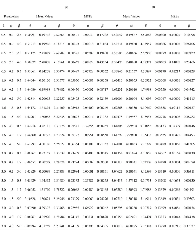
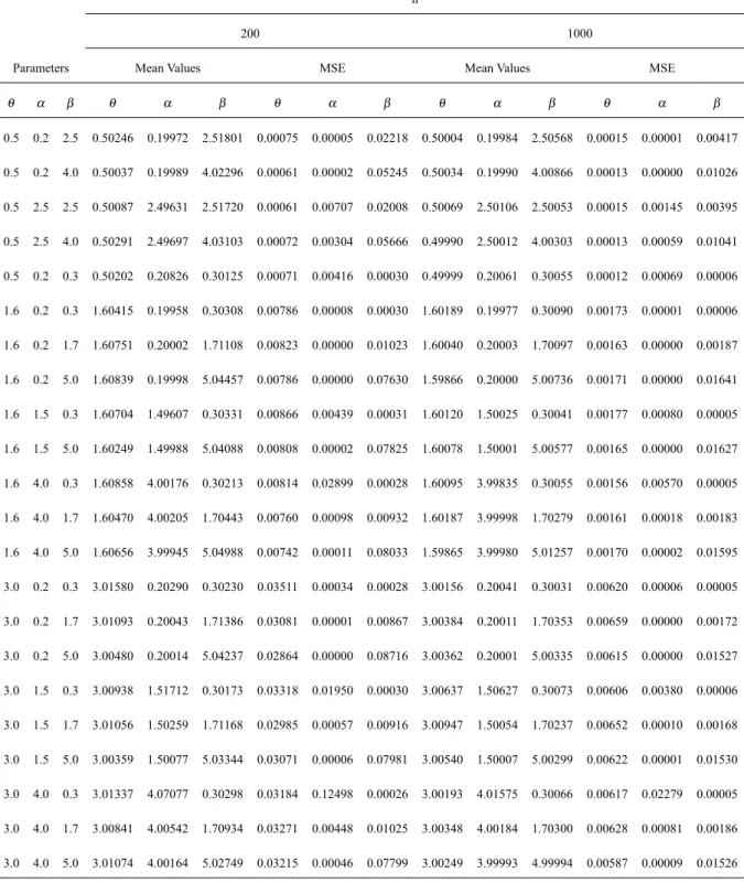
dif-ferent combinations of true parameter values in the first column of Tables II and III are adopted for the data generating process. Tables II and III list the mean values and mean square errors (MSEs) of the MLEs of the model parameters by taking sample sizesn=30,50,200and1,000. The figures in both tables indicate

7 - APPLICATIONS

We provide two applications of the LiW model to prove empirically its potentiality by comparing to the fits of other competitive models, namely: the Weibull Lindley (WLi) (Asgharzadeh et al. 2018), Weibull Fréchet (WFr) (Afify et al. 2016b), transmuted complementary Weibull geometric (TCWG) (Afify et al. 2014), Kumaraswamy Weibull (KwW) (Cordeiro et al. 2010), beta Weibull (BW) (Lee et al. 2007), gamma Weibull (GW) (Provost et al. 2011) and W distributions, whose pdfs (forx>0) are given in Appendix A.

In order to compare the fits of the LiW model with other competing distributions, we consider the Anderson-Darling(A∗)and Cramé r-von Mises (W∗) statistics. The two statistics are widely used to compare

non-nested models and to determine how closely a specific cdf fits the empirical distribution of a given data set. These statistics are given by

A∗=

9 4n2+

3 4n+1

n+1

n

∑

n

j=1(2j−1)log

zi 1−zn−j+1

and

W∗=

1 2n+1

(

∑

zi−

2j−1 2n

2

+ 1 12n

) ,

respectively, wherezi=F(yj)and theyj’s values are the ordered observations.

Data Set I: Exceedances of Wheaton River Flood

The data represent the exceedances of flood peaks (in m3/s) of the Wheaton River near Carcross in Yukon Territory, Canada. The data consist of 72 exceedances for the years 1958–1984, rounded to one decimal place (see Choulakian and Stephens 2001).

Data Set II: Failure Times of 84 Aircraft Windshield

The second data set consists of 84 failure times for a particular windshield device. These failures do not result in damage to the aircraft but do result in replacement of the windshield (Murthy et al. 2004).

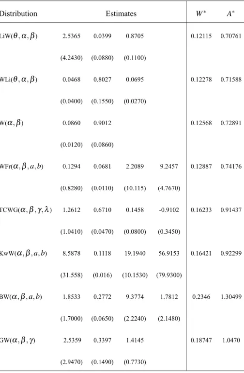
Tables IV and V list the values of the statisticsA∗ andW∗ for eight fitted models to these two data

sets. The MLEs and their corresponding standard errors (in parentheses) of the model parameters are also given in these tables. The figures in both tables reveal that the LiW distribution yields the lowest values of these statistics among the fitted models and then provides the best fit to both data sets. Hence, we prove empirically that the proposed distribution provides better fits in two applications than other six extended Weibull distributions with three and four parameters. There are too many models to fit and this fact really shows that the LiW distribution can be a good alternative for modeling survival data.

The figures in these tables are calculated using the MATHCAD program. In this program, we provide any initial values (in several cases from fits of special models) and then the program calculates the MLEs. After that, we update the initial estimates to obtain new values for the MLEs. This process continues up to obtain the final MLEs, which make the first derivatives of the log-likelihood function equal to zero.

TABLE II

The mean values and MSEs based on 1,000 simulations of the LiW. distribution.

n

30 50

Parameters Mean Values MSEs Mean Values MSEs

θ α β θ α β θ α β θ α β θ α β

0.5 0.2 2.5 0.50991 0.19792 2.62564 0.00501 0.00030 0.17232 0.50649 0.19867 2.57862 0.00300 0.00020 0.10098

0.5 0.2 4.0 0.51217 0.19906 4.18515 0.00493 0.00013 0.51064 0.50734 0.19860 4.14959 0.00286 0.00008 0.26106

0.5 2.5 2.5 0.51175 2.47809 2.62782 0.00521 0.05289 0.19608 0.50506 2.48636 2.56986 0.00279 0.02888 0.09129

0.5 2.5 4.0 0.50879 2.48038 4.19961 0.00467 0.01829 0.43254 0.50495 2.48680 4.12371 0.00303 0.01091 0.23466

0.5 0.2 0.3 0.51061 0.24238 0.31474 0.00497 0.05728 0.00262 0.50846 0.21737 0.30899 0.00270 0.02213 0.00129

1.6 0.2 0.3 1.64044 0.20130 0.31577 0.05970 0.00087 0.00258 1.62416 0.20055 0.30922 0.03668 0.00036 0.00127

1.6 0.2 1.7 1.64080 0.19998 1.79482 0.06436 0.00002 0.08717 1.63232 0.20010 1.74988 0.03550 0.00001 0.04742

1.6 0.2 5.0 1.62814 0.20005 5.22257 0.05475 0.00000 0.72139 1.61006 0.20004 5.14097 0.03047 0.00000 0.41215

1.6 1.5 0.3 1.64172 1.51804 0.31409 0.05912 0.04400 0.00249 1.62863 1.50330 0.30960 0.03558 0.02118 0.00127

1.6 1.5 5.0 1.62901 1.50058 5.22638 0.05627 0.00014 0.71332 1.60478 1.49987 5.15953 0.02978 0.00007 0.38982

1.6 4.0 0.3 1.62918 4.06111 0.31276 0.05541 0.32855 0.00265 1.61808 3.99504 0.31052 0.03133 0.14399 0.00146

1.6 4.0 1.7 1.64360 4.00722 1.77624 0.05722 0.00951 0.08558 1.61299 3.99800 1.75432 0.03555 0.00426 0.04493

1.6 4.0 5.0 1.63797 4.00106 5.25027 0.06354 0.00108 0.71757 1.62001 4.00063 5.13799 0.03489 0.00061 0.41305

3.0 0.2 0.3 3.08367 0.22157 0.31638 0.23409 0.00405 0.00245 3.04353 0.21084 0.30855 0.14662 0.00169 0.00130

3.0 0.2 1.7 3.06657 0.20248 1.78674 0.23794 0.00009 0.08300 3.04115 0.20141 1.74705 0.14390 0.00004 0.04079

3.0 0.2 5.0 3.05929 0.20089 5.27383 0.22984 0.00001 0.70851 3.04622 0.20041 5.12599 0.13519 0.00001 0.36311

3.0 1.5 0.3 3.05429 1.64512 0.31480 0.23332 0.21787 0.00255 3.04415 1.57312 0.30713 0.13708 0.10655 0.00130

3.0 1.5 1.7 3.06052 1.51710 1.78322 0.26068 0.00480 0.08165 3.03280 1.50993 1.74986 0.13679 0.00268 0.04491

3.0 1.5 5.0 3.10828 1.50621 5.25946 0.23379 0.00060 0.74276 3.02710 1.50318 5.14911 0.13649 0.00031 0.39503

3.0 4.0 0.3 3.07690 4.39372 0.31468 0.22985 1.66922 0.00262 3.05295 4.20288 0.30719 0.13699 0.84081 0.00134

3.0 4.0 1.7 3.08967 4.05920 1.79784 0.24145 0.03831 0.08628 3.03756 4.02491 1.74494 0.13823 0.02043 0.04438

TABLE III

The mean values and MSEs based on 1,000 simulations of the LiW distribution.

n

200 1000

Parameters Mean Values MSE Mean Values MSE

θ α β θ α β θ α β θ α β θ α β

0.5 0.2 2.5 0.50246 0.19972 2.51801 0.00075 0.00005 0.02218 0.50004 0.19984 2.50568 0.00015 0.00001 0.00417

0.5 0.2 4.0 0.50037 0.19989 4.02296 0.00061 0.00002 0.05245 0.50034 0.19990 4.00866 0.00013 0.00000 0.01026

0.5 2.5 2.5 0.50087 2.49631 2.51720 0.00061 0.00707 0.02008 0.50069 2.50106 2.50053 0.00015 0.00145 0.00395

0.5 2.5 4.0 0.50291 2.49697 4.03103 0.00072 0.00304 0.05666 0.49990 2.50012 4.00303 0.00013 0.00059 0.01041

0.5 0.2 0.3 0.50202 0.20826 0.30125 0.00071 0.00416 0.00030 0.49999 0.20061 0.30055 0.00012 0.00069 0.00006

1.6 0.2 0.3 1.60415 0.19958 0.30308 0.00786 0.00008 0.00030 1.60189 0.19977 0.30090 0.00173 0.00001 0.00006

1.6 0.2 1.7 1.60751 0.20002 1.71108 0.00823 0.00000 0.01023 1.60040 0.20003 1.70097 0.00163 0.00000 0.00187

1.6 0.2 5.0 1.60839 0.19998 5.04457 0.00786 0.00000 0.07630 1.59866 0.20000 5.00736 0.00171 0.00000 0.01641

1.6 1.5 0.3 1.60704 1.49607 0.30331 0.00866 0.00439 0.00031 1.60120 1.50025 0.30041 0.00177 0.00080 0.00005

1.6 1.5 5.0 1.60249 1.49988 5.04088 0.00808 0.00002 0.07825 1.60078 1.50001 5.00577 0.00165 0.00000 0.01627

1.6 4.0 0.3 1.60858 4.00176 0.30213 0.00814 0.02899 0.00028 1.60095 3.99835 0.30055 0.00156 0.00570 0.00005

1.6 4.0 1.7 1.60470 4.00205 1.70443 0.00760 0.00098 0.00932 1.60187 3.99998 1.70279 0.00161 0.00018 0.00183

1.6 4.0 5.0 1.60656 3.99945 5.04988 0.00742 0.00011 0.08033 1.59865 3.99980 5.01257 0.00170 0.00002 0.01595

3.0 0.2 0.3 3.01580 0.20290 0.30230 0.03511 0.00034 0.00028 3.00156 0.20041 0.30031 0.00620 0.00006 0.00005

3.0 0.2 1.7 3.01093 0.20043 1.71386 0.03081 0.00001 0.00867 3.00384 0.20011 1.70353 0.00659 0.00000 0.00172

3.0 0.2 5.0 3.00480 0.20014 5.04237 0.02864 0.00000 0.08716 3.00362 0.20001 5.00335 0.00615 0.00000 0.01527

3.0 1.5 0.3 3.00938 1.51712 0.30173 0.03318 0.01950 0.00030 3.00637 1.50627 0.30073 0.00606 0.00380 0.00006

3.0 1.5 1.7 3.01056 1.50259 1.71168 0.02985 0.00057 0.00916 3.00947 1.50054 1.70237 0.00652 0.00010 0.00168

3.0 1.5 5.0 3.00359 1.50077 5.03344 0.03071 0.00006 0.07981 3.00540 1.50007 5.00299 0.00622 0.00001 0.01530

3.0 4.0 0.3 3.01337 4.07077 0.30298 0.03184 0.12498 0.00026 3.00193 4.01575 0.30066 0.00617 0.02279 0.00005

3.0 4.0 1.7 3.00841 4.00542 1.70934 0.03271 0.00448 0.01025 3.00348 4.00184 1.70300 0.00628 0.00081 0.00186

TABLE IV

MLEs (standard errors in parentheses) and the statisticsW∗andA∗for data set I.

Distribution Estimates W∗ A∗

LiW(θ,α,β) 2.5365 0.0399 0.8705 0.12115 0.70761

(4.2430) (0.0880) (0.1100)

WLi(θ,α,β) 0.0468 0.8027 0.0695 0.12278 0.71588

(0.0400) (0.1550) (0.0270)

W(α,β) 0.0860 0.9012 0.12568 0.72891

(0.0120) (0.0860)

WFr(α,β,a,b) 0.1294 0.0681 2.2089 9.2457 0.12887 0.74176

(0.8280) (0.0110) (10.115) (4.7670)

TCWG(α,β,γ,λ) 1.2612 0.6710 0.1458 -0.9102 0.16233 0.91437

(1.0410) (0.0470) (0.0800) (0.3450)

KwW(α,β,a,b) 8.5878 0.1118 19.1940 56.9153 0.16421 0.92299

(31.558) (0.016) (10.1530) (79.9300)

BW(α,β,a,b) 1.8533 0.2772 9.3774 1.7812 0.2346 1.30499

(1.7000) (0.0650) (2.2240) (2.1480)

GW(α,β,γ) 2.5359 0.3397 1.4145 0.18747 1.0470

(a)

x

Density

0 1 2 3 4 5

0.0

0.1

0.2

0.3

0.4

0.5

LiW WLi KwW GW

(b)

x

Density

0 1 2 3 4 5

0.0

0.1

0.2

0.3

0.4

0.5

LiW BW TCWG WFr W

Figure 3 -The fitted densities for the:(a)LiW, WLi, KwW and GW models;(b)LiW, BW, TCWG, WFr and W models (data set I).

(a)

x

Density

0 10 20 30 40 50 60

0.00

0.02

0.04

0.06

0.08

0.10

0.12 LiW

WLi KwW GW

(b)

x

Density

0 10 20 30 40 50 60

0.00

0.02

0.04

0.06

0.08

0.10

0.12 LiW

BW TCWG WFr W

TABLE V

MLEs (standard errors in parentheses) and the statisticsW∗andA∗for data set II.

Distribution Estimates W∗ A∗

LiW(θ,α,β) 0.3036 0.9209 1.8846 0.05022 0.49507

(0.3138) (0.6552) (0.2465)

WLi(θ,α,β) 0.2311 3.0359 0.3104 0.07666 0.54281

(0.0819) (0.4246) (0.0214)

TCWG(α,β,γ,λ) 0.0188 0.9598 1.4081 0.6649 0.07758 0.57770

(0.0610) (0.7160) (2.7490) (0.294)

W(α,β) 0.3493 2.3744 0.08296 0.74365

(0.0170) (0.2100)

KwW(α,β,a,b) 14.4331 0.2041 34.6599 81.8459 0.18523 1.50591

(27.095) (0.0420) (17.5270) (52.0140)

WFr(α,β,a,b) 630.9384 0.3024 416.0971 1.1664 0.25372 1.95739

(697.942) (0.032) (232.359) (0.357)

BW(α,β,a,b) 1.3600 0.2981 34.1802 11.4956 0.46518 3.21973

(1.0020) (0.0600) (14.8380) (6.7300)

GW(α,β,γ) 2.3769 0.8481 3.5344 0.25533 1.94887

8 - CONCLUSIONS

In this paper, we propose a new three-parameter model, called the Lindley Weibull (LiW) distribution, which extends the Weibull (W) distribution. In fact, the LiW distribution is motivated by the wide use of the W distribution in many applied areas and also for the fact that the generalization provides more flexibility to analyze real data. The LiW density function can be expressed as a linear combination of the exponentiated-W (exp-exponentiated-W) densities. exponentiated-We derive explicit expressions for the ordinary and incomplete moments, moments of the (reversed) residual life, quantile and generating functions and order statistics. We discuss the max-imum likelihood estimation of the model parameters. Two applications illustrate that the proposed model provides consistently better fit than other competitive models. We hope that the new distribution will attract wider applications in reliability, engineering and other areas of research. Estimation of the model parame-ters under the bayesian paradigm is currently underway and will be reported in a separate article elsewhere. However, we must make a note of the fact under the Bayesian setting, that a non informative prior approach is essentially maximum likelihood estimation under the classical approach. In the absence of an appropriate conjugate prior, the choice of prior will be a challenging in such a setting. As a future work we will consider bivariate and multivariate extension of the LiW distribution. In particular with the copula based construction method, trivariate reduction etc.

ACKNOWLEDGMENTS

The authors are thankful to the Editor and the reviewers for their constructive comments and suggestions which greatly improved the current version.

REFERENCES

AFIFY AZ, CORDEIRO GM, BUTT NS, ORTEGA EMM AND SUZUKI AK. 2017. A new lifetime model with variable shapes for the hazard rate. Braz J Probab Stat 31: 516-541.

AFIFY AZ, CORDEIRO GM, YOUSOF HM, ABDUS S AND ORTEGA EMM. 2018. The Marshall-Olkin additive Weibull distribution with variable shapes for the hazard rate. Hacettepe J Math Stat 47: 365-381.

AFIFY AZ, NOFAL ZM AND BUTT NS. 2014. Transmuted complementary Weibull geometric distribution. Pak J Stat Oper Res 10: 435-454.

AFIFY AZ, YOUSOF HM, CORDEIRO GM, ORTEGA EMM AND NOFAL ZM. 2016. The Weibull Frechet distribution and its applications. J Appl Stat 43: 2608-2626.

ARYAL GR, ORTEGA EMM, HAMEDANI GG AND YOUSOF HM. 2017. The Topp-Leone generated Weibull distribution: regression model, characterizations and applications. Int J Stat Probab 6: 126-141.

ARYAL GR AND TSOKOS CP. 2011. Transmuted Weibull distribution: a generalization of the Weibull probability distribution. Eur J Pure Appl Math 4: 89-102.

ASGHARZADEH A, NADARAJAH S AND SHARAFI F. 2018. Weibull Lindley distribution. Revstat 16: 87-113.

CAKMAKYAPAN S AND OZEL G. 2017. The Lindley family of distributions: properties and applications. Hacettepe J Math Stat 46: 1-27.

CHOULAKIAN V AND STEPHENS MA. 2001. Goodness-of-fit for the generalized Pareto distribution. Technometrics 43: 478-484.

CORDEIRO GM, HASHIMOTO EM AND ORTEGA EMM. 2014a. The McDonald Weibull model. Stat J Theor Appl Stat 48: 256-278.

CORDEIRO GM, ORTEGA EMM AND DA CUNHA DCC. 2013. The exponentiated generalized class of distributions. J Data Sc 11: 1-27.

CORDEIRO GM, ORTEGA EMM AND SILVA GO. 2014b. The Kumaraswamy modified Weibull distribution: theory and applications. J Stat Comput Simul 84: 1387-1411.

ELBATAL I AND ARYAL G. 2013. On the transmuted additive Weibull distribution. Austrian J Stat 42: 117-132.

GHITANY ME, AL-HUSSAINI EK AND AL-JARALLAH RA. 2005. Marshall-Olkin extended Weibull distribution and its application to censored data. J Appl Stat 32: 1025-1034.

HANOOK S, SHAHBAZ MQ, MOHSIN M AND KIBRIA G. 2013. A Note on Beta Inverse Weibull Distribution. Commun Stat Theory Methods 42: 320-335.

KILBAS AA, SRIVASTAVA HM AND TRUJILLO JJ. 2006. Theory and Applications of Fractional Differential Equations Elsevier, 1st_{ed., Amsterdam, 540 p.}

LAI CD, XIE M AND MURTHY DNP. 2001. Bathtub-shaped failure rate life distributions. Handbook of Statistics 20: 69-104. LAI CD, XIE M AND MURTHY DNP. 2003. A modified Weibull distribution. IEEE Trans Reliab 52: 33-37.

LEE C, FAMOYE F AND OLUMOLADE O. 2007. Beta-Weibull distribution: some properties and applications to censored data. J Mod Appl Stat Methods 6(1): 173-186.

MEROVCI F AND ELBATAL I. 2013. The McDonald modified Weibull distribution: properties and applications. arXiv preprint arXiv:13092961. (In Press).

MUDHOLKAR GS AND SRIVASTAVA DK. 1993. Exponentiated Weibull family for analyzing bathtub failure-real data. IEEE Trans Reliab 42: 299-302.

MUDHOLKAR GS, SRIVASTAVA DK AND FREIMER M. 1995. The expnentiated Weibull family: a reanalysis of the bus-motor-failure data. Technometrics 37: 436-445.

MUDHOLKAR GS, SRIVASTAVA DK AND KOLLIA GD. 1996. A generalization of the Weibull distribution with application to the analysis of survival data. J of the Ameri Stat Associa 91: 1575-1583.

MURTHY DNP, XIE M AND JIANG R. 2004. Weibull Models. Hoboken, NJ, 1st_{ed., J Wiley & Sons, 408 p.} NADARAJAH S. 2009. Bathtub-shaped failure rate functions. Qual Quant 43: 855-863.

NADARAJAH S, CORDEIRO GM AND ORTEGA EMM. 2013. The exponentiated Weibull distribution: A survey. Stat Pap 54: 839-877.

NOFAL ZM, AFIFY AZ, YOUSOF HM AND CORDEIRO GM. 2017. The generalized transmuted-G family of distributions. Commun Stat Theory Methods 46: 4119-4136.

NOFAL ZM, AFIFY AZ, YOUSOF HM, GRANZOTTO DCT AND LOUZADA F. 2016. Kumaraswamy transmuted exponentiated additive Weibull distribution. Int J Stat Probab 5: 78-99.

PROVOST SB, SABOOR A AND AHMAD M. 2011. The gamma Weibull distribution. Pak J Stat 27: 111-131. SARHAN AM AND ZAINDIN M. 2009. Modified Weibull distribution. Applied Sciences 11: 123-136.

SHAHBAZ MG, SHAHBAZ SAND BUTT NM. 2102. The Kumaraswamy inverse Weibull distribution. Pak J Stat Oper 8: 479-489. SILVA GO, ORTEGA EMMAND CORDEIRO GM. 2010. The beta modified Weibull distribution. Lifetime DataAnal 16: 409-430. XIE M AND LAI CD. 1995. Reliability analysis using an additive Weibull model with bathtubshaped failure rate function. Reliab

Eng Syst Saf 52: 87-93.

XIE M, TANG Y AND GOH TN. 2002. A modified Weibull extension with bathtub failure rate function. Reliab Eng Syst Saf 76: 279-285.

YOUSOF HM, AFIFY AZ, ALIZADEH M, BUTT NS, HAMEDANI GG AND ALI MM. 2015. The transmuted exponentiated generalized-G family of distributions. Pak J Stat Oper 11: 441-464.

APPENDIX A:

The pdfs of the competitive fitted models are given by: WLi: f(x) = exp

−θx−(βx)α

(1+θ) h

αθ(βx)α+αβ(1+θ) (βx)α−1+θ2_(1+x)i_;

WFr: f(x) =abβ αβx−β−1exph−b α_xβin1−exph− α_xβio−b−1

×exp

−anexph− α_xβi−1o −b

;

TCWG: f(x) =αβ γβyβ−1nα(1−λ)−(α−αλ−λ−1)exph−(γy)βio

KwW: f(x) =abβ αβxβ−1exp

h

−(αx)βin1−exp

h

−(αx)βioa−1

×n1−n1−exph−(αx)βioaob−1;

BW: f(x) = _Bβ α_(a,β_b)xβ−1exph−b(αx)βin1−exph−(αx)βioa−1;

GW: f(x) =β αγ/β+1_xβ+γ−1_{exp −αx}β_{/Γ(1+γ/β);}