(Annals of the Brazilian Academy of Sciences)
Printed version ISSN 0001-3765 / Online version ISSN 1678-2690 http://dx.doi.org/10.1590/0001-3765201720160292
www.scielo.br/aabc
Thermodynamic bounds for existence of normal shock in compressible fluid flow in pipes
SERGIO COLLE
Laboratory of Energy Conversion Engineering and Energy Technology (LEPTEN), Department of Mechanical Engineering, Federal University of Santa Catarina (UFSC), Trindade, 88040-900 Florianópolis, SC, Brazil
Manuscript received on May 17, 2016; accepted for publication on December 19, 2016
ABSTRACT
The present paper is concerned with the thermodynamic theory of the normal shock in compressible fluid flow in pipes, in the lights of the pioneering works of Lord Rayleigh and G. Fanno. The theory of normal shock in pipes is currently presented in terms of the Rayleigh and Fanno curves, which are shown to cross each other in two points, one corresponding to a subsonic flow and the other corresponding to a supersonic flow. It is proposed in this paper a novel differential identity, which relates the energy flux density, the linear momentum flux density, and the entropy, for constant mass flow density. The identity so obtained is used to establish a theorem, which shows that Rayleigh and Fanno curves become tangent to each other at a single sonic point. At the sonic point the entropy reaches a maximum, either as a function of the pressure and the energy density flux or as a function of the pressure and the linear momentum density flux. A Second Law analysis is also presented, which is fully independent of the Second Law analysis based on the Rankine-Hugoniot adiabatic carried out by Landau and Lifshitz (1959).
Key words:Normal shocks in pipes, compressible fluid flow, gas dynamics, Second Law analysis.
INTRODUCTION
The study of the shock theory in fluid mechanics started with the pioneering work of (Rayleigh, 1899-1920) who discovered that in a steady-state compressible flow of an ideal gas in a straight pipe under the condition of constant linear momentum, defined byp+ρV2, there occurs a normal shock, whenever the fluid speed
reaches the sound speed. Rayleigh described the geometric loci of constant linear momentum in the Mollier diagram as a curve that became known as theRayleigh curve. Fanno (Shapiro 1953), in his doctor thesis, which was submitted to the Real Academy of Engineering of Genova in 1930, proposed a new approach to predict the normal shock in pipes, other than the one due to Rayleigh1. In his approach he considered the gas flow under constant energy density flux defined byh+V2/2. In both works, it is assumed that the mass
E-mail: [email protected]
flow density defined byj = ρV is constant. The geometric loci of states of constant values ofh+V2/2 as defined by Fanno became known as the Fanno curve. It is well known in gas dynamics that Rayleigh and Fanno curves can cross each other in two distinct points, one of which where the flow is subsonic and the other one where the flow is supersonic. It is hard to find in scientific journals any novelty concerning the theory on the normal shock in pipes, since there is a considerable number of papers and books devoted to the topic of gas dynamics, covering normal and oblique shock in compressible fluid flow, as well as its application to the design of nozzle, turbine blades and supersonic aircraft wings. The book of Anderson (2003) and the e-book of Bar-Meir (2013) report the state of the art of gas dynamics theory and applications to aerodynamics. However, it seems that few works have been published concerning the thermodynamic analysis of the normal shock in pipes. A remarkable analysis is presented in Landau and Lifshitz (1959) where the authors carried out a thermodynamic analysis focusing the normal shock in pipes based on the Hugoniot-Rankine adiabatic. In their work, based on the Second Law of Thermodynamics, they set down thermodynamic inequalities for both, weak and strong normal shocks. They also carried out a thermody-namic analysis of the Fanno flow, from which the Fanno curve is shaped in the entropy-pressure diagram. In spite the fact that the theory beneath the normal shock is well established, the author of the present paper carried out a thermodynamic analysis for the Rayleigh flow, from which, a theoretical duality for the Fanno flow and the Rayleigh flow is shown to exist. It is shown here that there exist a single state in the entropy -pressure diagram, at which the Fanno and Rayleigh curves become tangent. The existence of the tangency point enables one to establish a symmetric thermodynamic formalism which provides the basis to obtain a Second Law inequality. This inequality is expressed in terms of the entropy, either as a function of the pres-sure and the linear momentum density fluxjm =j(p+ρV2)or as a function of the pressure and the energy
density fluxje=j(h+V2/2), wherej=ρV is the mass flow density in the pipe, which is assumed to be
constant. The entropy inequality enables one to derive two independent inequalities, which are expressed in terms of the fluid specific heats, the isothermal compressibility coefficient, the adiabatic compressibility coefficient, and the thermal expansion coefficient. It is also shown that the entropy discontinuity arising from a weak normal shock implies the entropy discontinuity for a strong normal shock.
FANNO FLOW
In Landau and Lifshitz (1959), the authors set down thermodynamic propriety relationship for sonic and supersonic states, by assuming that the mass flow densityj =ρV and the energy flux densityh+V2/2are constant along the pipe axis. However, similar conditions can be found by assuming bothjand the energy
flux densityje =j(h+V2/2)constant. Definingxas the axial coordinate of a pipe andV as the average
velocity over the cross section of the pipe, it follows,
∂je
∂x
je,j =j ∂
∂x
h+V 2
2
je,j =j
"
∂h ∂x
je,j +j2v
∂v ∂x
je,j
#
whereV =jvandvis the fluid specific volume. Furthermore,dh=T ds+vdp, and therefore
∂h ∂x
je,j
= T
∂s ∂x
je,j
+ v
∂s ∂x
je,j
. On the other hand, ∂v
∂x
je,j = ∂v ∂p s ∂p ∂x
je,j + ∂v ∂s p ∂s ∂x
je,j
. These identities lead to
"
T+j2v ∂v ∂s p # ∂s ∂x
je,j +v
1 +j2 ∂v ∂p s ∂p ∂x
je,j
= 0 (1)
It is well known from thermodynamics that,∂v
∂s
p
= T α
cp . For gases this derivative is positive, since
the thermal expansion coefficientα= 1
v ∂v ∂T p
is also positive. Moreover,
j2 ∂v ∂p s = V 2 v2 ∂v ∂p s
= V2 v2
∂p ∂v s
=−V 2
c2
wherec2 =
∂p ∂ρ
s
=−v2
∂p ∂v
s
is the sound speed square for the fluid considered. The above identity can be expressed as follows,
1 +j2
∂v ∂p
s
= 1−V 2
c2 (2)
Eq. (1) gives the derivative of the pressure as follows,
∂p ∂x
je,j
= −
"
T +j2v ∂v ∂s p # ∂s ∂x
je,j
, v
1 +j2 ∂v ∂p s (3)
Since the fluid flow is irreversible one has,∂s
∂x
je,j
>0. By considering that the denominator of the
above equation does not vanish forV 6=c, Eq. (2) and Eq. (3) imply that
∂p ∂x
je,j
<0forV < cwhile
forV > c,
∂p ∂x
je,j
>0. The conclusion is that for a subsonic flow the pressure decreases downstream
while for a supersonic flow the pressure increases downstream. Eq. (1) enables one to write the following identity,
∂s ∂p
je,j = −v
1 +j2 ∂v ∂p s , "
T+j2v ∂v ∂s p # (4)
From Eq. (2) the above identity can be expressed as follows,
∂s ∂p
je,j = −v
1− V 2
c2
, "
T +j2v ∂v ∂s p # (5)
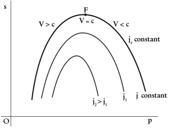
vanishes, which shows that the entropy reaches an extremum. These results allow one to conclude that the geometric loci of states of constantjein thes−pdiagram display a curve along which the entropy increases
up to the point where the flow is sonic, and decreases thereafter. By using analogous procedure of Landau and Lifshitz, the following identity can be obtained,
∂2s ∂p2
je,j
V=c
= −j2v
∂2v ∂p2
s , "
T +j2v
∂v ∂s
p #
(6)
The second derivative of the volume in the above equation can be reduced with the help of a Maxwell relation derived from the Gibbs thermodynamic potential, to obtain the following identity,
∂2v ∂p2
s
= ∂
∂p
∂v ∂p
s
= ∂
∂p(−ksv)s, whereks is the adiabatic compressibility coefficient. Thus the
following identity holds,
∂2v
∂p2
s
=v "
k2s−
∂ks ∂T
p αv cpT −
∂ks
∂p
T #
(7)
whereαis the thermal expansion coefficient. For a perfect gasks = 1/(kp)wherek=cpo/cvois the Poisson
coefficient, which is known to be constant. Therefore the derivative of ks respective to the temperature
vanishes. Thus Eq. (7) is reduced to the following expression,
∂2v ∂p2
s
=v
ks2+
1
kp2
>0 (8)
As remarked in (Landau and Lifshitz 1959), for most real gases of practical interest this derivative is known to be positive. Thus the second derivative given by Eq. (6) is negative at the point for whichV =c.
Therefore, the sonic state is the geometric locus of a maximum for the entropy as a function ofp, under the
condition of constant energy flux density. The above results allow one to justify the Fanno curve shape in thes−pdiagram as shown in Fig. 1 reported in the above mentioned reference. The identities given by Eq.
(1) to Eq. (6) are shown here to be equivalent to the respective identities reported in the above mentioned reference.
RAYLEIGH FLOW
The theory presented in the previous section, can be extended to the Rayleigh flow by assuming both,jand
the linear momentum densityjm =j(p+ρV2)constant. By replacingρV2=j2vinto the last equation it
follows,d(p+ρV2) =d(p+j2v) =djm. Thus the following identity holds,
dp+j2dv = 0 (9)
The above identity leads to the identity,∂p
∂x
jm,j +j2
∂v ∂x
jm,j
= 0. By replacing the volume
derivative by the identity given by,∂v
∂x
jm,j =
∂v ∂s
p
∂s ∂x
jm,j +
∂v ∂p
s
∂p ∂x
jm,j
the following identity is found,
∂p ∂x
jm,j
= −j2
∂v ∂s
p
∂s ∂x
jm,j
,
1 +j2
∂v ∂p
s
Figure 1 -Fanno curves in the entropy – pressure diagram.
From the above equation and Eq. (2), one can see that∂p
∂x
jm,j
is negative wheneverV < cand
pos-itive wheneverV > c. Therefore, the pressure decreases downstream whenever the fluid follow is subsonic
and it increases downstream whenever the fluid flow is supersonic. Equation (10) enables one to write the following,
∂s ∂p
jm,j
= −
1 +j2
∂v ∂p
s , "
j2
∂v ∂s
p #
(11)
As has been remarked earlier, the derivative∂v
∂s
p
is positive. It follows from the above equation and
Eq. (2) that∂s
∂p
jm,j
is positive wheneverV > cand negative wheneverV < c.
ForV = cEq. (2) implies that
∂s ∂p
jm,j
= 0. Thus, the entropy as a function ofpandjm reaches an
extremum at the state of sonic flow on the curve ofjmconstant. Analogous proof as given by Landau and
Lifshitz is reported in Colle (2015), to obtain the following identity,
∂2s ∂p2
jm,j
V=c
= −
∂2v ∂p2
s ,
∂v ∂s
p
(12)
As remarked earlier, the derivative ∂2v
∂p2
s
is positive. From the above identity it follows that
∂2s ∂p2
jm,j
<0. Thus, the entropy reaches its maximum as a function ofpunder the condition of
MAXIMUM ENTROPY THEOREM
In order to show the existence of a thermodynamic symmetry between Rayleigh flow and Fanno flow, in terms of the entropy either as a function of the pressure andjeor as a function of the pressure andjm, under
the condition of constant mass flow density, the following Lemma is proposed and proved.
Lemma: If a compressible steady-state axial flow of a gas in a pipe of constant cross section is adiabatic, then the entropy variation along the pipe axis is due to the variation of the linear momentum density flux along the pipe axis. Conversely, if the linear momentum density flux is constant along the pipe axis, then the entropy variation along the pipe axis is due to the heat flux at the boundary of the pipe cross section.
Proof: By assumingjconstant, we can write,
dje|j−vdjm|j =jd(h+V2/2)
j −jvd(p+ρV
2) |j
By the definitions ofjeandjm, the following differential expressions are obtained,
d je|j =d(h+j
2v2 /2)
j =dh+j
2vdv, and dj
m|j =d(p+j2v)|j =dp+j2dv
From these identities it follows,
d je|j−vd djm|j =j(dh+j
2vdv
)−jv(dp+j2dv) =j(dh−vdp) =jT ds
Thus the following thermodynamic identity holds,
dje|j−vdjm|j =jT ds (13)
From this identity, the following identities hold
∂je
∂x
j
−v
∂jm ∂x
j
=jT
∂s ∂x
j
(14)
The above equation implies the following identities,
∂jm
∂x
je,j
=−jT
∂s ∂x
je,j
/v (15)
∂je
∂x
jm,j =jT
∂s ∂x
jm,j
(16)
The first part of the lemma follows from Eq. (15). The second part of the lemma follows from Eq. (16), sincejmis constant while
∂s ∂x
jm,j
is due to the axial variation ofje, which by its turn is proportional to
the heat flux variation at the pipe cross section boundary. In other words, quasi-static heat income is required in order to maintainjm constant along the pipe axis downstream. However, it remains to be shown thatjm
decreases downstream. By the way, for the present case the First Law of thermodynamics, can be expressed by the following equation,
d dx
ρV
h+V
2
2
j
=
∂je
∂x
j
=−1
A I
Γ ˆ
The Second Law can be expressed as follows,
jT
∂s ∂x
j
=−1
A I
Γ ˆ
q·nˆldl+
1
A I
A
˙
φ−qˆ· ∇T T
dA (18)
whereAis the pipe cross section area, qˆis the heat flux vector, nˆl is the unit vector normal to the cross
section boundary curveΓ, andφ˙ is the fluid power dissipation per unit volume due to friction. From Eq. (14), Eq. (17), and Eq. (18) the following identity is obtained,
−v
∂jm ∂x
j
= 1
A Z
A
˙
φ−qˆ· ∇T T
dA (19)
Since from thermodynamicsqˆ· ∇T is known to be non-positive, the above equation implies that the
linear momentum density decreases withxdownstream.
Since Eq. (19) holds regardless to the fact that the flow is adiabatic or not, for an adiabatic flow one has,
−v
∂jm ∂x
j
= 1
A Z
A
˙
φ− qˆ· ∇T T
dA=jT
∂s ∂x
je,j
(20)
The above identity is equivalent to identity (15). In Eq. (19),qˆ· ∇T =−kc
dT dx
2
, wherekcis the
fluid thermal conductivity. It is remarkable that the integral of Eq. (19) vanishes if and only if the dissipation term vanishes in the case the flow is assumed to be isothermal. On the other hand, for high flow speed, the axial temperature gradient in both, Eq. (18) and Eq. (19), becomes much smaller than the viscous dissipation term. By disregarding the viscous dissipation term in favor of the heat flux term in Eq. (18), Eq. (19) implies thatjmbecomes constant. Thus Eq. (17) and Eq. (18) enable one to write the following identity,
∂je
∂x
jm,j =−1
A I
Γ ˆ
q·nldlˆ =jT
∂s ∂x
jm,j
(21)
The above identity is equivalent to identity (16). These equations show that the axial variation of both, the energy density flux and the entropy arise from the heat flux effect at the boundary, as stated in the second part of the Lemma.
Since the pressure is a function ofx, the following identity also holds,
∂je
∂p
j
−v
∂jm ∂p
j
=jT
∂s ∂p
j
(22)
The above equation implies the following identities,
∂jm
∂p
je,j
=−jT
v ∂s
∂p(p, je, j) (23)
∂je
∂p
jm,j
=jT∂s
It is remarkable that Eq. (13) suggests that the parametersje andjm can be regarded as independent
thermodynamic variables of the entropy function. Furthermore, the differential form of Eq. (13) enables one to write the following identities,
∂s ∂je
jm,j
= 1
jT (25)
∂s ∂jm
je,j
=− v
jT (26)
SinceT is always positive, Eq. (25) implies that the entropy increases with the increase of the energy
density flux, under constant linear momentum density flux. Eq. (26), by its turn shows that the entropy decreases with the increase of the linear momentum density flux, under constant energy density flux.
The proved lemma enables one to prove the following theorem:
Theorem: ”In a compressible steady-state fluid flow of a gas in a pipe of constant cross section area, for a given energy flux density, there exist a minimum linear momentum density flux below which a normal shock cannot occur. Conversely, for a given linear momentum density flux, there exist a maximum energy density flux above which a normal shock cannot occur”.
Proof: The proof of this theorem follows from the fact that at pointM of the state for whichV =cthe
following identity holds
∂s
∂p(p, je, j) = j
2
v
∂v ∂s
p ∂s
∂p(p, jm, j) , "
T+j2v
∂v ∂s
p #
(27)
This identity can be proved with the help of the following identity derived from calculus,
∂s
∂p(p, jm, j) = ∂s
∂p(p, je, j) +
∂s ∂je
p,j
∂je ∂p
jm,j
(28)
The definition ofjegives,
∂je ∂je
p,j
=j "
∂h ∂je
p,j
+j2v
∂v ∂je
p,j #
= 1
where
∂h ∂je
p,j
=T
∂s ∂je
p,j
and ∂v
∂je
p,j
=
∂v ∂s
p
∂s ∂je
p,j
From these three last identities it follows,
∂s ∂je
p,j
= 1
, j
"
T+j2v
∂v ∂s
p #
(29)
Analogous proof can be used to obtain the following identity
∂s ∂jm
p,j
= 1
, j3
∂v ∂s
p
The identity given by Eq. (27) is obtained by replacing in to Eq. (28), the derivative ∂je
∂p
jm,j by its
expression of Eq. (24), and the derivative∂s
∂je
p,j
by its expression given by Eq. (29). From Eq. (27)
one can see that the derivative ∂s
∂p(p, je, j)vanishes if and only if ∂s
∂p(p, jm, j)vanishes. Eq. (27) and the
results obtained in the previous sections, enable one to conclude that pointMis the point for which both, the
entropy expressed bys(p, je, j)and the entropy expressed bys(p, jm, j)reach an extremum. It remains to
be shown that at pointM,jmreaches a minimum whilejereaches a maximum as functions ofpfor constant j.
The second derivative of Eq. (22) leads to the following identity
∂2je
∂p2
j
−
∂v ∂p
j
∂jm ∂p
j
−v
∂2jm ∂p2
j
=j
∂T ∂p
s
∂s ∂p
j
+jT
∂2s ∂p2
j
(31)
Forjeconstant the above equation is reduced to
∂v ∂p
je,j
∂jm
∂p
je,j +v
∂2jm
∂p2
je,j =−j
∂T
∂p
s
∂s ∂p
je,j +jT
∂2s ∂p2
At pointM whereV =c, Eq. (23) implies that
∂jm ∂p
je,j
vanishes, since∂s
∂p
je,j
vanishes at the point considered. From the above expression of the second derivative it follows the identity
v
∂2jm ∂p2
=−jT
∂2s ∂p2
je,j
Since the entropy as a function ofpandjereaches a maximum forV =c, its second derivative with
respect topis negative. Therefore the second derivative of the left hand side of the above equation becomes
positive. This shows thatM is a point of minimum ofjmas a function ofpandjefor constantje.
Forjmregarded as constant, Eq. (24) shows that at pointM,
∂je ∂p
jm,j
vanishes, since ∂s
∂p(p, jm, j)
vanishes at the point considered, while Eq. (31) gives,
∂2je
∂p2
jm,j =j
∂T ∂p
s
∂s ∂p
jm,j +jT
∂s ∂p
jm,j
At the pointM the first derivative of the entropy vanishes and therefore one has,
∂2je
∂p2
jm,j =jT
∂2s ∂p2
jm,j
(32)
Since the entropy as a function of pandjm reaches a maximum forV = c, its second derivative is
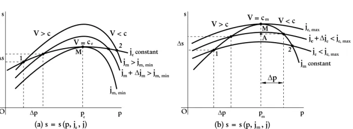
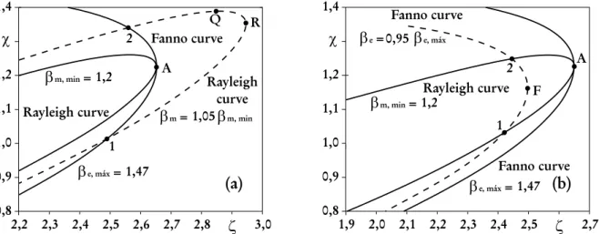
negative and therefore the second derivative of the left hand side of the above equation becomes negative. This shows thatM is a point of maximum ofjeas a function ofpandjmfor constantjm. Figures 2a and
Figure 2 - (a)Possible states arising from the intersection of Rayleigh curves with a given Fanno curve.(b)Possible states arising from the intersection of Fanno curves with a given Rayleigh curve.
The last step of the proof is to show that point M is a single tangency point of Fanno and Rayleigh
curves. By the way, Eq. (6) and Eq. (12) enables one to write the following inequality,
∂2s
∂p2
je,j
V=c >
∂2s
∂p2
jm,j
V=c
On the other hand, in the neighborhood of the tangency point for whichp = pe = pm, the Taylor
expansion ofs(pe, je, j)gives,s(pe±∆p, je, j)−smax(pe, je, j) =
∂2s ∂p2
je,j (∆p)2
2 , while the Taylor
expansion ofs(pm, jm, j) gives,s(pm±∆p, jm, j)−smax(pm, jm, j) =
∂2s ∂p2
jm,j (∆p)2
2 . From the above expressions it follows,
s(pm±∆p, je, j)−s(pm±∆p, jm, j) = "
∂2s
∂p2
je,j −
∂2s
∂p2
jm,j
#
pm (∆p)2
2 >0 (33)
The above inequality enable on to conclude that the convexity of the curve respective tos(p, jm, j)(the
Rayleigh curve) is greater than the convexity of the curve respective tos(p, je, j)(the Fanno curve). From
Eq. (33) it can be seen that as∆pvanishes,s(pm, jm, j) =s(pm, je,max, j)and s(pm, je, j) =s(pm, jm,min, j), as shown in Fig. 2.
TEMPERATURE INEQUALITY
An useful identity to derive an inequality related to the Second Law of thermodynamics can be obtained by casting Eq. (29) with the identity given by,
∂T ∂je
p,j
=
∂T
∂s
p
∂s ∂je
and the thermodynamic identity given by,∂v
∂s
p
= T vα
cp
. The following identity is found,
∂T ∂je
p,j
= 1
j(cp+j2v2α)
(34)
This identity enables one to conclude that the temperature increases by increasing the energy density flux, under constant pressure. Analogous proof with the help of Eq. (30) leads to the following identity
∂T ∂jm
p,j
= 1
j3vα (35)
This identity enables one to conclude that the temperature increases by increasing the linear momentum density flux under constant pressure.
The temperature as a function ofsandpgives,dT =
∂T
∂p
s dp+
∂T
∂s
p
ds, where
∂T
∂s
p
= T
cp and
∂T ∂p
s
= αvT
cp . Integrating the temperature differential between the states of(s1, p1)
and(s2, p2)it follows,
T2−T1 =
Z p2
p1
∂T
∂p
s1
dp+
Z s2
s1
∂T
∂s
p2
ds (36)
The derivative identity respective tojeformer to Eq. (34) enables one to write,
∂T ∂je
p,j
dje|p =
∂T ∂s
p
ds|p. Thus, the second term of Eq. (36) can be expressed by
Z je+∆je
je
∂T ∂je
p2,j
dje, for∆je<0. Eq. (34) implies that the derivative ofT with respect tojeis always
positive. From Eq. (36) one can conclude thatT2 > T1 wheneverp2 > p1. One can see from Eq. (34) and Eq. (36) that state (2) can be reached from state (2”) by increasing the energy density flux under constant pressure. The chosen integration path is shown in Figure 3.
Eq. (36) implies that the temperature of state (2”) shown in Figure 3, which has the same entropy of state (1), is greater than the temperature of the latter state. In other words, the inequality T2 > T1 holds wheneverp2 > p1, even if s2 = s1. Therefore the temperature inequality does not necessarily imply the entropy inequality.
THE MOLLIER DIAGRAM
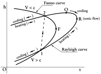
The thermodynamic equations expressed in terms of the independent variables je andjm can be used to
derive appropriate equations in order to express the entropy as a function of the enthalpy. Figure 4 illustrates the Fanno and the Rayleigh curves sketched in the well known Mollier diagram.
Figure 4 -Fanno and Rayleigh curves in the Mollier diagram.
THE ENTROPY AS A FUNCTION OFh,je, ANDj- FANNO CURVE
From calculus it follows
∂s ∂h
je,j =
∂s ∂p
je,j
,
∂h ∂p
je,j
(37)
while from thermodynamics one has,
∂h ∂p
je,j
=T
∂s ∂p
je,j
+v (38)
By replacing the derivative of the right hand side of the former equation by its expression given by Eq. (5), it follows,
∂h ∂p
je,j = T v
V2
c2 −1
, "
T+j2v
∂v ∂s
p #
+v
This derivative can also be expressed as follows
∂h ∂p
je,j
= v
" T V2
c2 +j 2
v
∂v ∂s
p #, "
T+j2v
∂v ∂s
p #
As remarked earlier, for gases,∂v
∂s
p
is known to be positive. This implies that both, the numerator and the denominator of Eq. (39) are positive. Thus, the inverse derivative
∂p ∂h
je,j = 1
,
∂h ∂p
je,j
becomes also positive. This identity implies that the pressure turns to be a monotonically increasing function ofh. Thus, one can write,s = s(p, je, j) = s(p(h, je, j), je, j) = s(h, je, j), so that this function preserves the shape of the Fanno curve in theh−sMollier diagram.
As can be seen in Figure 4, point F is the state for which the entropy reaches a maximum as a function ofhfor constantje. In fact, Eq. (37) shows that at pointF, for whichV =c, the derivative of the entropy
as a function ofpfor constantjevanishes. Thus, the derivative of the entropy as a function of the enthalpy
for constantjealso vanishes.
THE ENTROPY AS A FUNCTION OFh,jm, ANDj- RAYLEIGH CURVE
From calculus it follows
∂s ∂h
jm,j =
∂s ∂p
jm,j
,
∂h ∂p
jm,j
(40)
while from thermodynamics one has∂h
∂p
jm,j
=T
∂s ∂p
jm,j
+v, where
∂s ∂p
jm,j
is given by Eq. (11). The inverse of the derivative given by Eq. (40) is given by the identity,
∂h ∂s
jm,j =
∂h ∂p
jm,j
,
∂s ∂p
jm,j
(41)
The above identities and the identity given by Eq. (11) enables one to obtain the following identity,
∂h ∂s
jm,j = −T
αV2−cp
1− V 2
c2
cp
1− V 2
c2
(42)
ForV different fromc, the denominator of the above equation is non-vanishing. As can be verified,
the above derivative vanishes forV = VQ, the solution of the algebraic equation given by,αV2−cp(1−
V2/c2) = 0. This equation gives,
VQ/c= q
cp/(cp+αc2) (43)
The pointQshown in Fig. 4 represents the state for which the derivative given by Eq. (42) vanishes. For
the particular case of a perfect gas, it can be verified that Eq. (43) is reduced to the well known correlation,
VQ/c= 1/
√
k. By replacingcpobtained from Eq. (43) into Eq. (42), the following identity is found
∂h ∂s
jm,j
= T
VQ2
c2 −
V c2
VQ2
c2 1−
V2 c2
(44)
The inverse of the above derivative is expressed as follows
∂s ∂h
jm,j =
1−V 2
c2
VQ2
c2 T
VQ2
c2 −
V c2
As shown by Eq. (43),VQ/c < 1. Therefore, for V = c Eq. (45) leads to
∂s ∂h
jm,j
= 0, which is the necessary condition for point R shown in Fig. 4 to be a point of maximum. Equation (44), by its
turn shows that the derivative∂h
∂s
jm,j
vanishes at the pointQshown in the same figure, which is the
necessary condition for this point to be a point of maximum. Equation (44) enables one to conclude that for
V < VQandV < c, the derivative
∂h ∂s
jm,j
is positive, which means the enthalpy increases by increasing the entropy. In other words, the enthalpy increases with the heat income and, therefore, the flow is heated. For any point located between pointQand pointRwhereV > VQandV < c, the derivative
∂h ∂s
jm,j becomes negative, which means the flow is cooled. For any point located at the inner branch of the Rayleigh curve,V > candV > VQ, and therefore the derivative
∂h ∂s
jm,j
becomes positive, which means the flow is heated.
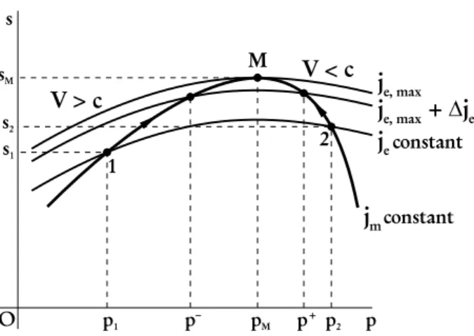
THE SECOND LAW INEQUALITY
The entropy change in the neighborhood of point M of maximum of the entropy, as shown in Fig. 2b,
can be expressed in terms of the independent variablespandje, along the curve ofjmconstant. Since the
first derivative∂s
∂p
je,j
vanishes at pointM, the Taylor expansion of the entropy up to the second order
derivatives evaluated at pointM, can be expressed as follows
∆s(p, je, j)|jm = (46)
=
∂s ∂je
p,j
∆je|jm + 1 2
∂2s ∂p2
je,j
(∆p)2+
∂2s ∂p∂je
j
∆je|jm∆p+ 1 2
∂2s ∂je2
p,j
(∆je|jm) 2
In the above equation∆je|jm becomes constrained on the curve ofjmconstant. The identity given by Eq. (13) leads to,∆je|jm =jT∆s(p, je, j)|jm. On the other hand, thought
∂s ∂p
jm,j
vanishes at pointM,
the Taylor expansion ofs(p, jm, j)in terms ofpin the neighborhood of this point is reduced to the following
identity,
∆s(p, je, j)|jm = 1 2
∂2s ∂p2
jm,j
(∆p)2 (47)
The last two identities lead to,∆je|jm = jT 1 2
∂2s ∂p2
jm,j
(∆p)2. Since the entropy reaches a maximum
at pointM , its second derivative in this expression is negative and therefore∆je|jm becomes negative, as assumed earlier. Moreover∆s(p, je, j)|jm is equal to∆s(p, jm, j)|je, for both are equal to the length of the segmentAMshown in Fig. 2b. By replacing∆je|jm by its last expression and∆s(p, je, j)|jmgiven by Eq. (47) into Eq. (46), the following algebraic equation of second degree in terms of∆pis found,
The coefficientsA,B, andCevaluated at pointMare given as follows,
A=−j 2T2
8
∂2s ∂je2
p,j
∂2s ∂p2
2
jm,j
(48)
B =−jT
∂2s ∂je∂p
∂2s ∂p2
jm,j
(49)
C= 1 2
"
∂2s ∂p2
jm,j −
∂2s ∂p2
je,j
#
−jT2
∂s ∂je p,j
∂2s ∂p2
jm,j
(50)
By taking the derivative of Eq. (29) with respect toje, by reducing the obtained equation with the help
of the identity, ∂
∂je p,j = ∂s ∂je p,j ∂ ∂s p
, and by replacing the derivative∂s
∂je
p,j
by its expression of Eq. (29), the following identity is found
∂2s ∂je2
p,j = − " ∂T ∂s p
+j2
∂v ∂s
2
p
+j2v
∂2v ∂s2 p #, j2 "
T+j2v ∂v ∂s p #3 (51)
The second derivative in the numerator of the above equation can be replaced by the identities,
∂ ∂s ∂v ∂s p = ∂ ∂T ∂v ∂s p ∂T ∂s p = ∂ ∂T αT v cp p T cp
The term of the last equality can be expanded in the form
∂2v
∂s2
p
= T v
cp2
(
α+α2T+T " ∂α ∂T p
−cpα
∂cp ∂T p #) (52)
Eq. (51) and Eq. (52) enable one to express Eq. (48) as follows
A=−
T3
8cp
∂2s ∂p2
2
jm,j
(
1 +j 2v2
cp "
α+T ∂α ∂T p # +j 2v2T α
cp "
2α− 1 cp ∂cp ∂T p #) "
T+j2v
∂v ∂s
p
#3 (53)
In the above equation,j2v2 =V2 =c2while from thermodynamics it is known that,c2 = vcp
cvkT. Thus
the above equation can also be expressed as follows,
A= 1 8
∂2v ∂p2
s
2
cp T2α2v2
(
1 + v
cvkT "
α+T ∂α ∂T p #
+ αT v
cvkT "
2α− 1 cp ∂cp ∂T p #)
1 + αv
cvkT
3 (54)
For the particular case of an ideal gas, for whichα = 1
T, the expression into the first bracket of the
numerator of the above equation vanishes, while the remaining terms are reduced to the following,
1 + αT v
cvkT "
By replacingα,c, andkT, this expression can be reduced to,
1
cvo
cpo+R− RT
cpo dcpo
dT
As the author has verified, this expression is positive for all ideal gases currently reported in thermo-dynamics textbooks.
By taking the derivative of Eq. (4) with respect to parameterje, at pointM the following identity holds,
∂2s ∂je∂p
=−jv ∂
2v
∂p∂s , "
T +j2v ∂v ∂s p #2 (55)
where, ∂2v
∂p∂s = ∂
∂s(−ksv)p =− " v ∂ks ∂s p
+ks ∂v ∂s p #
,∂ks ∂s p = ∂ks ∂T p ∂T ∂s p , ∂v ∂s p
= αT v
cp
>0, and
∂T ∂s p = T cp
>0. From these identities it follows
∂2v
∂p∂s =− T v cp " ksα+ ∂ks ∂T p # (56)
Equations (49), (55), and (56) enable one to write constantBas follows
B= cp
cvkTαT
∂2v ∂p2
s "
ksα+ ∂ks ∂T p #,
1 + αv
cvkT 2
(57)
For the particular case of a perfect gas,ks= 1/kp, wherekis the Poisson coefficient. Thus,
∂ks ∂T
p
= 0. By considering that the second derivative in the numerator of Eq. (57) is positive, for this particular case considered, the constantB becomes positive. One can see from Eq. (57) that the constantB
is positive if and only if the inequality,ksα+
∂ks ∂T
p
>0holds.
By replacing the derivatives in Eq. (50) by their expressions given by Eq. (6) and Eq. (12), the following equation is found,
C =− T 2
∂2v ∂p2 s , ∂v ∂s p "
T +j2v ∂v ∂s p # (58)
By replacing the derivative∂v
∂s
p
= αT v
cp in the above equation it follows
C =− 1 2
cp αT v
∂2v ∂p2
s
1 + αv
cvkT
(59)
Since the second derivative of the above equation is assumed to be positive, the coefficientCbecomes
unconditionally negative. The roots of the formerly obtained algebraic equation in terms of are given by, ∆p− = −(B +√B2−4AC)/(2A) and ∆p+ =
−(B −√B2−4AC)/(2A). Let us assume that
ksα+
∂ks ∂T
p
has,√B2−4AC < B, sinceC <0. Thus,∆p−becomes positive. Since by definition∆p− =p−−p
M, p−becomes grater thanpM, which cannot be the case. Therefore,Amust be positive. Thus Eq. (54) implies
the inequality given below
1 + v
cvkT "
α+T
∂α ∂T
p #
+ αT v
cvkT "
2α− 1 cp
∂cp ∂T
p #
>0 (60)
SinceCis negative one has√B2−4AC > B, which implies∆p+ > 0and∆p− <0as expected. Moreover,∆p++ ∆p− =−B/A. It follows from this inequality that|∆p−|>∆p+. On the other hand,
Eq. (47) leads to,s−−s
M = ∆s−|jm = 1 2
∂2s ∂p2
jm,j
(∆p−)2, and
s+−sM = ∆s+|jm = 1 2
∂2s ∂p2
jm,j
(∆p+)2. These equations enable one to write the following,
s+−s−=s+−s
M−(s−−sM) =
1 2
∂2s ∂p2
jm,j
[(∆p+)2−(∆p−)2] (61)
Since at pointMthe second derivative of the entropy is negative, the above equation implies,s+> s−.
This inequality shows that the entropy increases during the transition of a weak shock, from the supersonic state ofs− to the subsonic state ofs+. Conversely, by assuming the Second Law inequality to hold for a
weak shock, as is currently assumed, Eq. (61) clearly implies the inequality,(∆p−)2 > (∆p+)2. As can
be shown, this inequality leads to,B√B2−4AC > 0and therefore, B > 0. From Eq. (57) follows the inequality,ksα+
∂ks
∂T
p >0.
From the identity given by Eq. (25), for the states ofs− ands+on the curve of constantjm one has,
∂s ∂je
−
jm,j
= 1
jT−and
∂s ∂je
+
jm,j
= 1
jT+. It should be taken into account that along the curve of constant
jm, for both states,s(p, jm, j) =s(p, je, j)and therefore in each branch of the curve given bys(p, jm, j),
the later equality leads to an implicit function ofjm,je, andp, for constantj. As Fig. 5 shows, for a given
value ofje, the curve of constantjmcrosses the curve of constantjein two distinct points corresponding to
two states, one of which defined byp−, which is a supersonic state and the other one defined byp+, which
is a subsonic state.
The former derivatives of the entropy enable one to write the following inequality
∂s ∂je
−
jm,j
= 1
jT− >
1
jT+ =
∂s ∂je
+
jm,j
(62)
for Eq. (36) givesT+
−T−>0forp+> p−ands+≥s−.
By multiplying both sides of inequality (62) by an arbitrarily small(−∆je|jm)>0, the following inequality is obtained,
sM −s−≈
∂s ∂je
−
jm,j
(−∆je|jm)>
∂s ∂je
+
jm,j
Figure 5 -Integration path for inequality (63).
The above inequality impliess+ > s−. On the other hand, by integrating the left hand side of inequality
(62) from state (1) to state ofs−and the right hand side of the same inequality from the state of to state (2)
with respect to the variablejealong the path shown in Fig. 1 it follows
s−−s
1 =
Z je,max+∆je
je
∂s ∂je
−
jm,j
dje=
Z je,max+∆je
je
1
jT−dje>
>
Z je,max+∆je
je
1
jT+dje=
Z je,max+∆je
je
∂s ∂je
+
jm,j
dje=s∗−s
2
where∆je = ∆je|jm < 0. This inequality gives,s2 > s1+ (s +
−s−) > s
1 and therefore,s2 > s1. The above inequality shows that as∆jevanishes, as shown in Fig. 5 both,s−ands+become equal tosM, and
therefore the above inequality is reduced to the following
sM −s1 =
Z je,max
je
∂s ∂je
−
jm,j
dje >
Z je,max
je
∂s ∂je
+
jm,j
dje=sM −s2 (63)
The above inequality also implies s2 > s1. These results enable one to conclude that the entropy discontinuity arising from a weak shock implies an entropy discontinuity for a strong shock.
EVALUATION OF THE TANGENCY POINT
At the tangency point the following equations must be imposed
∂s ∂p
(p, jm, j) = 0 (64)
∂s ∂p
(p, je, j) = 0 (65)
s(p, jm, j) =s(p, je, j) (66)
Equation (64) can be written as
∂s ∂p
v
+
∂s ∂v
p
∂vm ∂p
jm,j
From the definition ofjmit follows
vm = (jm/j−p)/j2 (68)
Equation (65) can be written as
∂s ∂p
v
+
∂s ∂v
p
∂ve ∂p
je,j
= 0 (69)
From the definition ofjeit follows
ϕ=h(p, ve) +j2ve/2−je/j= 0 (70)
The derivative∂ve ∂p
je,j
in Eq. (69) is determined by the identities arising from calculus,
∂ve
∂p
je,j,ϕ
=−
∂ϕ ∂p
v,je,j
,
∂ϕ ∂v
p,je,j
,
∂ϕ ∂p
v,je,j =
∂h ∂p
v
, and
∂ϕ ∂v
p,je,j =
∂h ∂v
p
+j2v.
By replacing these derivatives into Eq. (69) it follows
"
∂h ∂v
p
+j2v #
∂s ∂p
v
−
∂h ∂p
v
∂s ∂v
p
= 0 (71)
On the other hand, from thermodynamics one has,
∂s ∂v
p
= cp
αvT ,
∂s ∂p
v
= cvkT
αT , dh=T ds+vdp ,
∂h ∂p
v
=T
∂s ∂p
v
+v= cvkT
α +v ,
∂h ∂v
p
=T
∂s ∂v
p
= cp
αv
Furthermore, Eq. (68) gives,∂vm
∂p
jm =−1
j2. By casting these identities with Eq. (71) the following identity is obtained
j2vmcvkT −cp = 0 (72)
This identity can also be obtained from Eq. (67). Therefore, at the tangency point the following equations must be satisfied
p+j2v−jm/j= 0 (73)
h(p, v) +j2v2/2−je/j= 0 (74)
j2vcvkT −cp = 0 (75)
These equations can be simultaneously solved in term ofp,v, andjefor a specified value ofjmor in
for,j2v2 =V2andc2=cpv/(cvkT). The details of the analytical solutions obtained for the particular case
of a perfect gas are given in the Appendix.
Another interesting identity to show thatjeandjmplay the role of independent variables can be derived
from the Jacobian of these parameters respective topandv, as defined by,
J
je, jm p, v
=
∂je
∂p
v,j
∂jm ∂v
p,j
−
∂je
∂v
p,j
∂jm ∂p
v,j
(76)
where∂je ∂p
v,j
=j
∂h ∂p
v
,∂je ∂v
p,j
=j "
∂h ∂v
p
+j2v #
,∂jm ∂p
v,j
=j,
∂jm ∂v
p,j
=j3,
∂h ∂v
p
= cp
αv, and
∂h ∂p
v
= cvkT
α +v. By replacing the above derivatives in the Jacobian given by Eq.
(76) it follows,
J
je, jm p, v
= j(j 2vcvkT
−cp)
αv (77)
It is remarkable that this Jacobian vanishes at the pointM, for Eq. (75) holds at this point. This means
that at pointM,jm andjebecome conjugated, as shown by the theorem proved here.
ANALYTICAL EXAMPLE FOR A PERFECT GAS
In order to illustrate the analysis presented in this paper, the particular case of a perfect gas will be presented. For a perfect gas, the enthalpy can be expressed byh=kpv/(k−1), wherek=cpo/cvois assumed equal
to 1,4. The physical variables can be replaced by the dimensionless variables, α = p/po, µ = j2v/po, ζm = (sm −som)/R,ζe = (se−som)/R = (se−soe)/R+ (soe−som)/R, wherese = s(p, je, j), sm = s(p, jm, j), andsoe andsom are the values of the entropy at an arbitrary chosen state given by po
andvo. The dimensionless enthalpy is defined by χ = hj2/po. Let us define also,βm = jm/(jpo) and
βe =jje/p2o. The corresponding dimensionless equations respective to equations presented in the previous
section are given in the Appendix. Fig. 6a shows the Fanno and Rayleigh curves in a dimensionless entropy - pressure diagram, for the case for whichβmis specified.
In Fig. 7,βm = 1,05βm,min and βe = 0,95βe,max were chosen in order to fit the curves in a
reduced diagram size. In the present case it is found,χA= 1,225,χR= 1,164,αQ= 0,6388,χQ= 1,389, ζQ = 2,846, and
VQ
c =
1 √
k.
The curves are plotted forβm = 1,2, for whichβe,max = 1,47andαe = 0,5are found. For the sake of comparison, the curve ofβe = 0,8βe,max is also plotted. Fig. 2b shows the Fanno and Rayleigh
curves for the case for whichβeis specified. The curves are plotted forβe= 1,47, for whichβm,min= 1,2 and αm = 0,5 are found. For the sake of comparison, the curve of βm = 1,1βm,min is also plotted.
Figure 6 - (a)Limiting Rayleigh curve for a given Fanno curve.(b)Limiting Fanno curve for a given Rayleigh curve.
Figure 7 - (a)Limiting Rayleigh curve for a given Fanno curve in the Mollier diagram.(b) Limiting Fanno curve for a given Rayleigh curve in the Mollier diagram.
CONCLUSIONS
Fanno flows. The theoretical results are graphically illustrated for the particular case of a perfect gas in both, thes−pand the Mollier diagram.
ACKNOWLEDGMENTS
The author is indebted to Ministry of Science and Technology for the researcher fellowship of Conselho Nacional de Desenvolvimento Científico e Tecnológico (CNPq). The author is grateful to his doctor student Allan R. Starke for his help with the computation of the equations. The author is also greatful to the support provided by project ANEEL/PETROBRAS No. PD-0553-0023/2012.
REFERENCES
ANDERSON JD. 2003. Modern compressible flow: with historical perspective, 3rded., McGraw-Hill.
BAR-MEIR G. 2013. Fundamentals of Compressible Flow Mechanics, version 0.4.9.8. Free e-book. COLLE S. 2015. Lectures on Classical Thermodynamics: Volume V - Compressible Fluid Flow (in por-tuguese), Edition of the Departament of Mechanical Engineering – Federal University of Santa Catarina, Florianópolis, Brazil, ISBN 978-85-916577-5-9.
LANDAU LD AND LIFSHITZ EM. 1959. Mechanics of Fluids, 1st ed., London: Pergamon Press. RAYLEIGH JWS. 1899-1920. Scientific Papers. 6 Vols, Cambridge, England.
SHAPIRO AH. 1953. The Dynamics and Thermodynamics of Compressible Fluid Flow. Vol. 1, Ronald Press.
APPENDIX
The enthalpy of a perfect gas can be expressed ash=kpv/(k−1). By this definition Eq. (74) becomes
k k−1
pv+ j
2v2
2 −
je
j = 0 (78)
From Eq. (75) followsj2vkT −k= 0wherekT = 1/pand therefore
p=j2v/k (79)
By replacingvfrom its expression given by Eq. (73) in the above equation it follows
pm =jm/[j(k+ 1)] (80)
By combining this equation with Eq. (79) one has
vm =kjm/[j3(k+ 1)] (81)
From the equation of the sound speed given by,c2=kpv, Eq. (79), and Eq. (80) it follows
cm=kjm/[j2(k+ 1)] (82)
From Eq. (78) follows
ve= 1
j2
s
k k−1
2
p2+ 2jje−
k k−1
p
By replacingvefrom the above equation in Eq. (79) it follows
pe
√ 2
k r
k−1
k+ 1
p
jje (84)
By eliminatingpe(=pm)from Eq. (80) and Eq. (84) the following function relatingjmandjeis found
jm =
√ 2
k j p
k2−1p
jje (85)
From Eq. (79) and Eq. (84) follows
ve=
√ 2
j2
r k−1
k+ 1
p
jje (86)
From the sound speed equation given byc2 =kpv, Eq. (84), and Eq. (86) it follows
ce =√2
r k−1
k+ 1
r je
j (87)
By dividing both sides of Eq. (73) bypoone has,jm/(jpo) =p/po+j2v/po. By defining the
dimen-sionless variablesβm=jm/(jpo),α=p/po, andj2v/po, Eq. (68) is reduced to,βm =α+µ, from which
comes
µm(α, βm) =βm−α (88)
whereµm =j2vm/po,µom =j2vom/po, andµom =βm−1, and thereforeβm >1andvm >1. Eq. (88)
impliesα < βm. Equation (78) can be reduced to the dimensionless form,βe=
k k−1
αµ+µ 2
2 where
βe=jje/po2is dimensionless. Solving the former equation in terms ofµone has,
µe(α, βe) =
s
k k−1
α2+ 2βe−
k k−1
α (89)
whereµe = j2ve/po, so that the above equation implies,βe > 0. By makingve = vm, Eq. (81) and Eq.
(86) give, kjm
j3(k+ 1) = √
2
j2
r k−1
k+ 1
p
jje, from which it follows, jm
j =
√ 2
k p
k2−1p
jje. By dividing
both sides of this equation bypo, the following dimensionless function relatingβeandβmis found
βm= √
2
k p
k2−1p
βe (90)
At the point of maximum of both,s(p, jm, j)ands(p, je, j), Eq. (80) and Eq. (84) give respectively
αm = βm
(k+ 1) (91)
αe= √
2
k r
k−1
k+ 1
p
βe (92)
The entropy function can be expressed as follows,
By replacingTandToin terms of the pressure and volume it follows
sm(p, jm, j) =som+cpoln[pvm/(povom)]−Rln(p/po) (93)
wherevmis expressed by Eq. (68) andvomis expressed by the same equation in the form
vom = (jm/j−po)/j2 (94)
In the same way,
se(p, je, j) =soe+cpoln[pve/(povoe)]−Rln(p/po) (95)
whereveis expressed by Eq. (83) andvom is expressed by the same equation in the form
voe=
1
j2
s
k k−1
2 p2
o+ 2jje−
k k−1
po
(96)
The dimensionless entropies are defined byζm= (sm−som)/R, and
ζe= (sm−som)/R= (se−soe)/R+ (soe−som)/R
Thus, Eq. (93) and Eq. (95) can be expressed by their respective dimensionless forms as follows
ζm(α, βm) =
k k−1
lnαµm(α, βm)
µm(1, βm)
−lnα (97)
ζe(α, βm) = ∆ζe+
k k−1
lnαµe(α, βe) µe(1, βe)
−lnα (98)
where∆ζe= (soe−som)/R,µm(α, βm)is expressed by Eq. (88) andµe(α, βe)is expressed by Eq. (89).
Two cases are analyzed as follows.
Case (a) - The parameterβm >1is specified
From Eq. (90) one hasβe,max=βm2k2/[2(k2−1)], and from Eq. (91) one hasαm=βm/(k+ 1). The
contact condition for the entropy curves given bysm andse, for the present case is assured by the equality ζm(αm, βm) =ζe(αm, βe,max). From this equation, Eq. (97), and Eq. (98) it follows
∆ζe(αm) =
k k−1
lnµm(αm, βm)µe(1, βe,max) µm(1, βm)µe(αm, βe,max)
(99)
The contact of the curve of constantβewith the curve of constantβmis assured by expressing Eq. (98)
as follows
ζe(α, βe) = ∆ζe(αm) +
k k−1
ln αµe(α, βe) µe(1, βe,max)
−lnα (100)
whileζm(α, βm)is expressed by Eq. (97).
From Eq. (90) one hasβm,min= √
2
k p
k2−1p
βe, and from Eq. (92) one hasαe= √
2
k r
k−1
k+ 1
p βe.
The contact condition for the entropy curves is assured by the equalityζm(αe, βm,min) =ζe(αe, βe). From
this equation, Eq. (97), and Eq. (98) it follows
∆ζe(αe) =
k k−1
lnµm(αe, βm,min)µe(1, βe)
µm(1, βm,min)µe(αe, βe)
(101)
The contact of the curve of constantβewith the curve of constantβmis assured by expressing Eq. (97)
as follows
ζm(α, βm) =
k k−1
ln αµm(α, βm)
µm(1, βm,min)
−lnα (102)
whileζe(α, βe)is expressed by Eq. (98).
The pointQlocated on the Rayleigh curve as shown in Fig. 4 is determined by Eq. (86) given in the
same reference. For a perfect gas,VQ/cs = 1/
√
k. By replacingVQ =jvQin the preceding equation one
has,jvQ/cs = 1/√k. By replacing the sound speedcsfrom its expression of Eq. (82) in the last equation
one has,
j3vQ(k+ 1)/jm =
√
k
In terms of the dimensionless variables the above equation is reduced to the following equation,
(βm−αQ)/βm =
√
k/(k+ 1) (103)
This equation givesαQ=βm(1 +k−
√
k)/(k+ 1).
The dimensionless enthalpy is defined as
χ=hj2/po2
From the expressions ofµandαone has,
χ=kµα/(k−1)
By the definitionµandα, at the pointQ, this equation leads to the following equation