PETRI NET MODEL DECOMPOSITION - A Model Based Approach Supporting Distributed Execution -

(1)

Anik´

o Katalin Horv´

ath da Costa

PETRI NET MODEL

DECOMPOSITION

- A Model Based Approach Supporting

Distributed Execution

-Disserta¸c˜ao apresentada para obten¸c˜ao do Grau de Doutor em

Engenharia Electrot´ecnica, Especialidade de Sistemas Digitais,

pela Universidade Nova de Lisboa, Faculdade de Ciˆencias e

Tecnologia

(2)

(3)

Acknowledgments

First of all, I would like to thank my supervisor, Professor Lu´ıs Gomes, for creating the conditions for my work to be done, and for being a good friend and colleague besides just being my supervisor.

I am grateful to Professor Steiger Gar¸c˜ao for giving me the opportunity to work in Portugal and to develop a carrier at the Faculty of Science and Technology of the New University of Lisbon.

Thanks to Jo˜ao Paulo Barros, for having interesting debates about ideas, and giving me good advice, and encouragement.

To Paulo Barbosa for helping me formalize the net splitting operation, and for his believing in my work and his encouragement to keep working.

To Regina Frei for revising my English writing and being such a good friend.

To Tiago Reis for the implementation of the first version of the Splitting tool, and other master thesis students such as Ricardo Ferreira, Rog´erio Rebelo, Henrique Ferreira, who used the modules generated by the splitting tool in their master thesis implementations, in this way contributing to the validation of its correctness.

To ´Oscar Ribeiro for helping me with the latex template.

To all my colleagues who encouraged me to keep going forward by having good conversations.

To all my friends and acquaintances in Portugal, in Hungary, and in the Czech Republic, who somehow contributed to me being the person I am today.

And last but not least, I would like to thank my parents M´aria and J´ozsef, my husband Henrique, and my son Pedro, for their support and love.

(4)

(5)

Abstract

Model-based systems development has contributed to reducing the enormous difference between the continuous increase of systems complexity and the improvement of methods and methodologies available to support systems development.

The choice of the modeling formalism is an important factor for success-fully increasing productivity. Petri nets proved to be a suitable candidate for being chosen as a system specification language due to their natural sup-port of modeling processes with concurrency, synchronization and resource sharing, as well as the mechanisms of composition and decomposition. Also having a formal representation reinforces the choice, given that the use of verification tools is fundamental for complex systems development.

This work proposes a method for partitioning Petri net models into con-current sub-models, supporting their distributed implementation. The IOPT class (Input-Output Place-Transition) is used as a reference class. It is ex-tended by directed synchronous communication channels, enabling the com-munication between the generated sub-models. Three rules are proposed to perform the partition, and restrictions of the proposed partition method are identified.

It is possible to directly compose models which result from the parti-tioning operation, through an operation of model addition. This allows the re-use of previously obtained models, as well as the easy modification of the intended system functionalities.

(6)

(7)

Resumo

O desenvolvimento de sistemas baseados em modelos tem vindo a contribuir para reduzir a enorme diferen¸ca entre o aumento continuado observado na complexidade dos sistemas e os melhoramentos dos m´etodos e metodologias dispon´ıveis para suportar o seu desenvolvimento.

A escolha do formalismo de modela¸cão é um factor importante para o sucesso do aumento da produtividade. As redes de Petri (RdP) mostraram-se como mostraram-sendo um candidato adequado para mostraram-ser escolhido como linguagem de especifica¸cão de sistema devido ao suporte natural a mecanismos de mod-ela¸cão de concorrência, sincroniza¸cão e partilha de recursos, bem como a mecanismos de composi¸cão e decomposi¸cão. Também o facto de ter uma representa¸cão formal refor¸ca a escolha, dado permitir o recurso a ferramen-tas de verifica¸cão, fundamentais para encarar o desenvolvimento de sistemas complexos.

Este trabalho propõe um método de parti¸cão de modelos de RdP em sub-modelos concorrentes, permitindo suportar a sua execu¸cão distribu´ıda. Como classe de referência utiliza-se a classe IOPT (Input-Output Place-Transition), à qual se adicionaram canais de comunica¸cão s´ıncrono direccionados, per-mitindo a comunica¸cão entre os sub-modelos gerados. São propostas três re-gras para realizar a parti¸cão, bem como identificadas as restri¸cões ao método de parti¸cão proposto.

´

E poss´ıvel realizar a composi¸cão directa de modelos resultantes da opera¸cão de parti¸cão através de uma opera¸cão de adi¸cão de modelos, permitindo re-utilizar módulos obtidos previamente, bem como alterar facilmente as fun-cionalidades pretendidas para o sistema.

(8)

(9)

List of Figures

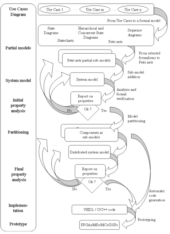
1.1 From models to code through model partitioning and mapping. 6

1.2 The interaction between a sender and a receiver [BACP95]. . . 8

1.3 The sender and the receiver modeled as objects [BACP95]. . . 9

1.4 Sender - Receiver connected through synchronous channels. . . 10

1.5 Space state graph of Sender - Receiver system models pre-sented in Figures 1.2 and 1.4. . . 10

1.6 Respective marking of the states of Figure 1.5. . . 11

1.7 Sender - Receiver connected through a communication node. . 12

1.8 Space state graph of the distributed Sender - Receiver system model presented in Figure 1.7. . . 13

1.9 Respective marking of the states of Figure 1.8. . . 14

2.1 Four-layered MDA architecture . . . 30

2.2 Methodology overview . . . 34

2.3 The development environment architecture; tool overview. . . 37

3.1 Isolated (a), Connected (b) and Strongly connected (c) nets. . 43

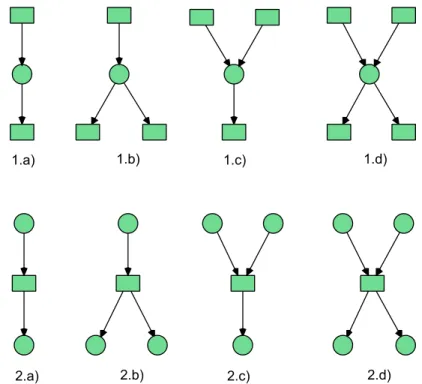
4.1 The identified eight different situations . . . 62

4.2 Rule #1 . . . 64

4.3 Rule #2 . . . 65

4.4 Rule #3 . . . 67

4.5 A typical conflict situation . . . 68

4.6 Simplified Rule #1 and Rule #2. . . 87

4.7 Simplified Rule #3. . . 88

(14)

5.2 Composition of modules: (a) System divided into two mod-ules; (b) Replication of one module and introduction of an

interconnection module . . . 94

5.3 Composition of modules: (a) The three subnets to be com-posed; (b) The result of the addition; (c) The equivalent de-composition net segment using Rule #1 . . . 96

5.4 Composition of modules resulted by applying Rule #2 . . . . 97

5.5 Composition of modules: (a) The initial net segment where Rule #3 will be applied; (b) The split net segment; (c) The equivalent composable net segments . . . 99

5.6 Composition of modules resulted by applying Rule #3 . . . . 100

5.7 Interconnection module nets: (a) for broadcast communica-tion; (b) for mutual exclusion, (c) for balanced communication discipline . . . 101

5.8 Broadcasting from one sender to two receivers . . . 103

6.1 N-cell FIFO system model [GBC05c]. . . 106

6.2 Coloured Petri net Model. . . 107

6.3 The IOPT Petri net model of the system controller [CGB+_{08]. 109} 6.4 Result of the splitting operation [CGB+_08]. _{. . . 111}

6.5 Result of the cutting nodes removal. . . 113

6.6 Result of the splitting operation considering t1 i and t7 i as the cutting set. . . 114

6.7 The composed controllers . . . 115

6.8 A composition with two robots between the first two conveyors 117 6.9 Three wagon system. . . 119

6.10 The global system model. . . 119

6.11 The six sub-models. . . 121

6.12 Model of the controller for the 1st wagon. . . 122

6.13 Model of the controller for the 2nd wagon. . . 122

6.14 Model of the controller for the 3rd wagon. . . 123

6.15 The distributed model. . . 125

6.16 The distributed model. . . 126

6.17 Addable models of the wagon controllers. . . 127

6.18 The distributed controller of the 4 wagon system. . . 128

6.19 Parking lot with one entrance and one exit area . . . 130

(15)

LIST OF FIGURES

6.21 Distributed controllers: (a) Entrance Zone, (b) Exit Zone, (c) Parking Area . . . 132 6.22 The composable models of the parking lot controllers. . . 133 6.23 The distributed model of the parking lot with two Entrance

(16)

(17)

Part I

(18)

(19)

Chapter 1 Introduction

Summary

This chapter gives an introduction to the research work pre-sented in this thesis, covering the motivation and defining the objectives.

1.1 Embedded Systems

Embedded systems constitute a very wide class of systems. There is no formal definition for them. However, in the literature, several definitions are avail-able, most of them defining embedded systems in terms of what they are not and giving examples of how the term is used. For example in [Hea02], “An embedded system is a microprocessor-based system that is built to control a function or range of functions and is not designed to be programmed by the end user in the same way that a PC is.” In the embedded system glossary [Bar99, Bar09] we can find the following definition for embedded system: “A combination of computer hardware and software, and perhaps additional me-chanical or other parts, designed to perform a dedicated function.” In some cases, embedded systems are part of a larger system or product, as in the case of an antilock braking system in a car.

Based on the above cited descriptions, it is possible to say that an embed-ded system is a part of a more complex system in which it is physically in-corporated, as its designation suggests. Embedded systems are usually built to control a given physical environment, composed of some electrical and/or electronic devices with which the embedded system has direct interaction, and mechanical equipment with which it has indirect interaction. Thus, to guarantee the interaction with the environment, there are several sensors and actuators included in the system [GF09]. Practically, all electronic devices we use in daily live can be considered as embedded systems; for example cell phones, microwaves, washing machines etc. The following characteristics are generally considered as the most important for an embedded system:

• An embedded system is usually developed to support a specific function for a given application.

• Embedded systems are expected to work continuously; they must op-erate while the bigger system is also operating.

• An embedded system should keep a permanent interaction with the environment in which it is inserted. This means that it has to respond to different stimuli, whose order and timing is unpredictable.

(21)

1.1. Embedded Systems

In [Cos03] embedded system is characterized as reactive system with ca-pability for real-time data processing.

Over the last decades of the 20th century the semiconductor technol-ogy has been continuously growing and technoltechnol-ogy was improved. This im-provement at chip level has made it possible to implement more and more functionalities on one chip, which in turn caused an increase of the system complexities at an almost exponential rate. Therefore, the traditional devel-opment of embedded system design or just system design, where the systems were designed directly at hardware or software low level, is no more feasible. This leads us to what is usually called the productivity gap generated by the disparity between the rapid increase of design complexity in comparison to that of design productivity. One solution to this problem is to raise the level of abstraction within the systems design process. For this reason the

Computer Aided Design (CAD) tools play a very important role. Some of the most important features of a specification language which can be used for embedded systems design with a CAD tool include the following [Hea02]:

• Hierarchy (behavioral and structural);

• State oriented behavior;

• Event-handling;

• Concurrency;

• Synchronization and communication;

• Executability;

• Readability;

• Portability and flexibility;

• Appropriate model of computation.

It is difficult to find any formal language which is capable of meeting all these requirements.

(22)

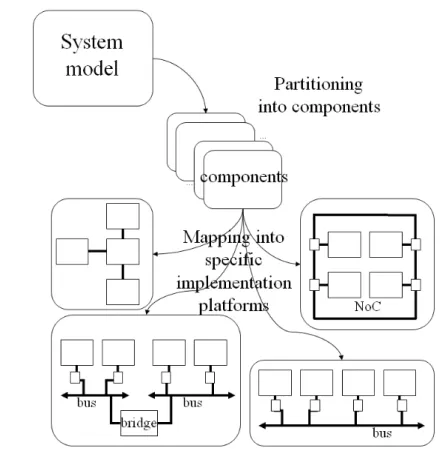
Figure 1.1: From models to code through model partitioning and mapping.

1.2 Motivation

As embedded systems are complex systems, the use of models for system analysis and system specification can facilitate the communication between developer teams and other people who are involved in system development -from the implementation and tester group to the end users.

It follows that using model based development in embedded systems de-sign can contribute to reducing the productivity gap, because beside the better communication between the several groups of people involved, it is possible to use automatic code generators.

(23)

1.2. Motivation

• The first phase, which consists of defining the system model;

• The second phase, where a set of components is built. In terms of Model Based Development, a component is also a model. The set of components is obtained based on the partitioning of the initial model into a set of concurrent sub-models;

• Finally, the third phase, where each component is mapped to a specific implementation platform.

Several distinct modeling formalisms have already proved their adequacy for embedded systems design supporting a model-based development approach [GBC05a]. Among them, we emphasize the use of control-based formalisms, where state-based formalisms play a major role. These formalisms include state diagrams, hierarchical and concurrent state diagrams, statecharts, se-quence diagrams and Petri nets.

Speaking about embedded systems is necessary to emphasizes that those systems are intrinsically composed by several components. Some of those components are commercially available components, like IPs (Intellectual Property) or libraries which the designer can use as a black box. Using the above mentioned formalism, these components can be represented in the system model as a node with several access points, which represent the communication between the system and the component.

(24)

p1 p2 p3 p4 p5 p6 p7 p8

t1 : SWork t2 : SendMsg t3 : ReceiveAck t4 : ReceiveMsg t5 : SendAck t6 : RWork p1 : SReady,S p2 : SWait,S p3 : SOk,S

p4 : Message,MSG p5 : Ack,MSG p6 : RReady,R p7 : RMsgReceived,R p8 : ROk,R

t2

t3 t5

t4

t6

t1

_N

Figure 1.2: The interaction between a sender and a receiver [BACP95].

global system model can bring benefits; it can, for instance, be used for system property verification purposes.

Several methods to deal with Petri net decomposition are available in the literature. However, most of them are based on introducing specific semantics for the communication nodes. A simple example (from [BACP95]) illustrates the interaction between a sender and a receiver, as presented in Figure1.2. For this simple example, it is intuitive to consider two components, one as-sociated with the sender, and the other one with the receiver. Places p4 and

p5 model the communication between the two components. Places p4 and

p5 should be included in the cutting set, allowing the splitting of the model. For example the proposals by Bruno et al. [BACP95] led to a concurrent application development environment, where the concept of objects supports the implementation of components. In this proposal, the splitting of the ini-tial net is accomplished through a set of places, and communication support depends on a target operating system or communication infrastructure (for instance, TCP could be used to support communication among objects). The models to be executed in parallel are presented in Figure 1.3.

(25)

1.2. Motivation t1 t2 t3 t4 t5 t6 p1 p2 p3 p6 p7 p8 p4 p4 p5 p5

Figure 1.3: The sender and the receiver modeled as objects [BACP95].

destination object. An output place is drawn as a circle with a triangle in-scribed. Input places receive tokens from the other objects, and put them into a queue for consumption. An input place is drawn as a double circle. This means that it is necessary to consider special semantics for executing the model and common verification methods are not applicable.

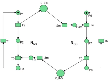
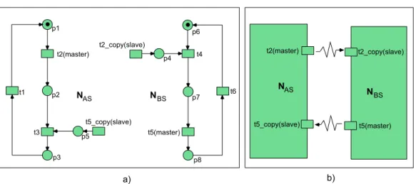
However, using transitions as interface nodes it is possible to avoid the definition of specific semantics for the interface nodes. Taking into account the presented example from [BACP95] it is possible to obtain the solution presented in Figure 1.4 (using the set of Rules presented in this thesis). It has to be stressed that the model N of Figure 1.2 is behaviorally equivalent to the models NAS and NBS of Figure 1.4 as long as the synchronous firing

of transitions T2 and t2m, andT5 and t5m are guaranteed.

In practical terms, the splitting of the initial model into two components is accomplished by considering P4 and P5 in the cutting set and relying on the usage of transitions with synchronous channels. The input transitions of the cutting place are duplicated in order to be included within both com-ponents. Taking the cutting set node P4 as an example, the consequence of the technique is the splitting of transition t2 at the initial model N into two transitions T2 and t2m at the models NAS and NBS, linked through a

(26)

Figure 1.4: Sender - Receiver connected through synchronous channels.

(27)

1.2. Motivation

(28)

Figure 1.7: Sender - Receiver connected through a communication node.

transition can be seen as a graphical convenience to identify components, as, from the execution point of view, it is completely equivalent to the initial model.

However, considering a distributed execution of the components, it means that each of them is executed on a different platform where it is not possible to use the same execution time domain (clock), and it is therefore necessary to include a communication module between the components. This module can be represented at a higher level as a Petri net place between the transitions

T2 and t2m, and T5 and t5m respectively, as shown in Figure 1.7.

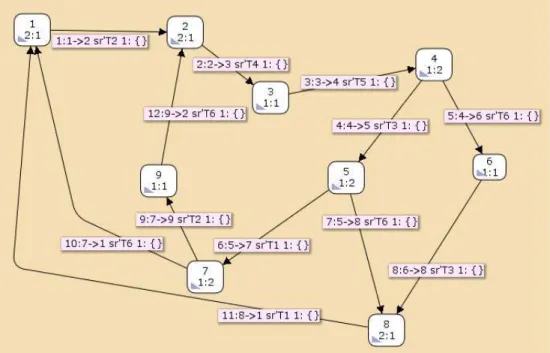
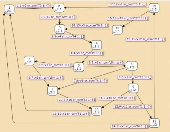
To demonstrate that both models (the initial model and the model with distributed execution) have the same behavior in terms of transitions fir-ing and place markfir-ing, we analyze the space state graph of both models, represented in Figures 1.5, 1.6, 1.8, and 1.9.

(29)

1.2. Motivation

(30)

(31)

1.3. Problem Statement

state 2 in the initial system model, and state 13 has the same marking as state 9 in the initial system.

In general, all global marking states of the initial model have a correspon-dence with some marking state in the distributed model.

For the initial system model, the firing sequence for returning to the initial state is the following: T2, T4, T5 followed by T3, T6, T1 in any possible order being T1 fired after T3. For the distributed model, the firing sequence is: T2, t2m, T4, T5 than t5m, T6, T3, T1 in any order being T3 fired after t5m, and T1 fired after T3. Observing these firing sequences, it can be assumed that to obtain the initial marking, the partial order of the firing sequence is the same in both cases.

1.3 Problem Statement

Considering the Petri net as a system specification language for embedded systems development, and considering that there are several classes of Petri nets, the questions are: which class of Petri nets is most suitable for embed-ded system modeling, how to split the system model into components, and how to reuse the obtained components for system modeling?

The answer for the first question was already given. Considering the re-active part of the system, without data processing, the Petri nets class con-sidered as the reference is the Input-Output Place-Transition (IOPT) Petri net[GBCN07] which was proposed in order to include the input and output signals/events of the system into the model.

This thesis intends to answer the remaining questions, namely:

• How to split the global system model into components which can be seen as independent system modules supporting distributed execution of the initial model?

• How to extend the IOPT Petri net class in order to include the com-munication between the sub-models?

(32)

1.4 Objectives

The main objective of this work is to propose a method to be used for Petri net model decomposition in order to obtain several sub-models which can be executed as independent components. In particular, this thesis proposes a net operation to be used within the IOPT Petri net class. Moreover the class is extended with directed synchronous communication channels in order to include an explicit way of communication between the resulting components in the model.

Additionally, this thesis indicates how to use the resulting components for model composition when the objective is to build a distributed system where several components with the same behavior can be identified.

Most of the known Petri net decomposition methods are based on prop-erty preservation and the communication between the obtained sub-models is done using specific semantics as mentioned in the previous subsections.

Our objective is to avoid new definitions and usage of specific semantics for communication between the sub-models. One goal is to benefit from semantics associated to the input/output signals and events defined within IOPT Petri nets. However, the questions of (1) solving conflict situations, (2) synchronizing processes and (3) proving that the decomposed model has the same behavior as the initial model, still remain.

Instead of focusing on the property preservation as the most of the other decomposition methods do, our main drive is in the behavior preservation, it means that the space state graph for both models (the initial and the decomposed) should keep the same partial order traces.

1.5 Contribution

This thesis introduces a new Petri net operation, named Net Splitting, that allows the splitting of a Petri net into several subnets. The resulting components can be deployed into heterogeneous implementation platforms. The communication between the components is represented through directed synchronous communication channels. These channels are attached to tran-sitions which can be seen as interface trantran-sitions. Also the algorithmic rep-resentations of the splitting rules that were used for implementing a support tool for the operation are provided.

(33)

1.5. Contribution

published during this work period. The article lists are organized in four groups, according to their relation with the topic of this thesis. All articles were published after being approved in a peer-reviewing process. All lists are presented in reverse chronological order.

The articles in the following list present the direct results from the work explained in this thesis, and were presented in international workshops and conferences, mostly by the author of this thesis.

1. [CBG+_{10] “Properties preservation in distributed execution of Petri} nets models”; Anik´o Costa, Paulo Barbosa, Lu´ıs Gomes, Franklin Ra-malho, Jorge Figueiredo, Antˆonio Junior; DoCEIS’10;

2. [CG09] “Petri net partitioning using net splitting operation”; Anik´o Costa, Lu´ıs Gomes; INDIN’2009;

3. [CG07c] “Petri net Splitting Operation within Embedded Systems Co-design”; Anik´o Costa, Lu´ıs Gomes; INDIN’2007;

4. [CG07a] “Module Composition within Petri Nets Model-based Devel-opment”; Anik´o Costa, Lu´ıs Gomes; SIES’2007;

5. [CG07b] “Parti¸c˜ao de redes de Petri integrada em metodologia de co-design de sistemas embutidos”; Lu´ıs Gomes, Anik´o Costa; REC’2007; 6. [GC06a] “Petri nets as supporting formalism within Embedded Systems

Co-design”; Lu´ıs Gomes, Anik´o Costa, - SIES’2006;

7. [CG06] “Partitioning of Petri net models amenable for Distributed Ex-ecution”; Anik´o Costa, Lu´ıs Gomes, - ETFA’2006.

The focus of the articles in the following list is not on the work presented in this thesis itself; however, the results of this thesis play an important role in these articles because theNet Splitting operation is applied to various case studies.

(34)

2. [FCG10] “Interliga¸c˜ao intra- e inter-circuito de componentes especifica-dos com Redes de Petri”; Ricardo Ferreira, Anik´o Costa, Lu´ıs Gomes; REC’2010;

3. [BRF+_{10] “Semantic Equations for Formal Models in the Model-Driven} Architecture”; Paulo Barbosa, Franklin Ramalho, Jorge Figueiredo, Anik´o Costa, Lu´ıs Gomes, Antˆonio Junior; DoCEIS’10;

4. [OCG09] “Configurador de plataformas espec´ıficas em Co-design de Sistemas Embutidos”; Jo˜ao Oliveira, Anik´o Costa, Lu´ıs Gomes; REC’2009;

5. [BCF+_{09] “Modeling Complex Petri Nets Operations in the} Model-Driven Architecture”; Paulo Barbosa, Anik´o Costa, Jorge Figueiredo, Frankilin Ramalho, Lu´ıs Gomes, Antˆonio Junior; IECON’2009;

6. [BRdF+_{09] “Checking Semantics Equivalence of MDA Transformations} in Concurrent Systems”; Paulo Barbosa, Franklin Ramalho, Jorge Fi-gueiredo, Antˆonio Junior, Anik´o Costa, Lu´ıs Gomes; JUCS 2009; 7. [CGB+_{08] “Petri nets tools framework supporting FPGA-based}

con-troller implementations”; Anikó Costa, Lu´ıs Gomes, João Paulo Bar-ros, João Oliveira, Tiago Reis; IECON’2008;

8. [GCBL07] “From Petri net models to VHDL implementation of digital controllers”; Lu´ıs Gomes, Anik´o Costa, Jo˜ao Paulo Barros, Paulo Lima; IECON’2007.

The following list includes articles which resulted from collaborative work done to define the underlying methodology for embedded systems develop-ment and the IOPT Petri net class:

1. [GBCN07] “The Input-Output Place-Transition Petri Net Class and Associated Tools”; Lu´ıs Gomes, Jo˜ao Paulo Barros, Anik´o Costa, Ri-cardo Nunes; INDIN’2007;

2. [GBC07] “Petri Nets Tools and Embedded Systems Design”; Lu´ıs Gomes, Jo˜ao Paulo Barros, Anik´o Costa; PNSE’07;

(35)

1.6. Structure of the Dissertation

4. [GBC+_{05d] “Formal methods for Embedded Systems Co-design: the} FORDESIGN project”; Lu´ıs Gomes, Jo˜ao Paulo Barros, Anik´o Costa, Rui Pais, Filipe Moutinho; ReCoSoC’05;

5. [GBC+_{05b] “Towards Usage of Formal methods within Embedded} Sys-tems Co-design”; Lu´ıs Gomes, Jo˜ao P.Barros, Anik´o Costa, Rui Pais, Filipe Moutinho, - ETFA’2005.

The following list of articles include papers which reflect the early prepa-ration phase of this work.

1. [GC06b] “Removing ill-structured arcs in Hierarchical and Concurrent State Diagrams”; Lu´ıs Gomes, Anik´o Costa, - ETFA’2006;

2. [CGFS06] “Internal event removal in Hierarchical and Concurrent State Diagrams”; Anik´o Costa, Lu´ıs Gomes, Helder Francisco, Bruno Silva, - DESDes’06;

3. [GC05b] “Statechart based component partitioning in hardware/software co-design”; Lu´ıs Gomes, Anik´o Costa; Jornadas sobre Sistemas Recon-figur´aveis (REC 2005);

4. [GBC05a] “Modeling Formalisms for Embedded Systems Design”; Lu´ıs Gomes, Jo˜ao Paulo Barros, Anik´o Costa; “Embedded Systems Hand-book”;

5. [GC05a] “Hardware-level Design Languages”; Lu´ıs Gomes, Anik´o Costa; “The Industrial Information Technology Handbook”;

6. [GBC05c] “Structuring Mechanisms in Petri Net Models: From spec-ification to FPGA based implementations”; Lu´ıs Gomes, Jo˜ao Paulo Barros, Anik´o Costa; “Design of embedded control systems”.

1.6 Structure of the Dissertation

This section provides an overview of how this dissertation is organized. The structure of the document is described and each chapter is briefly summa-rized.

(36)

Part I includes chapter 1 to 3 and presents the background of this thesis; Part II includes chapter 4 to 7 and presents the contribution of this thesis.

Chapter 2 presents existent methodologies for embedded systems design. It starts by describing computation models and the evolution of sys-tem development. This is followed by a brief description of the model based development and the presentation of the Model Driven Architec-ture approach. Finally, the FORDESIGN project development flow is explained. This project served as base for the work which led to this thesis.

Chapter 3 introduces Petri nets, the underlying formalism. Low-level Petri nets are characterized and theInput-Output Place-Transition Petri net class, which was defined within the FORDESIGN project and used as system specification language presented. At the end of this chapter, a brief overview of the existing Petri net decomposition methods is given. Chapter 4 is the core of this thesis, describing the proposed Net Spliting Operation. First, the IOPT Petri net class is extended to include communication channels, calledDirected Synchronous Communication Channel. Afterwards, an informal description of the splitting rules is provided, followed by formal definitions and the implementation algo-rithms description. The chapter ends with a description of the valida-tion possibilities of the operavalida-tion.

Chapter 5 presents a method for reusing the resulting models to build a more complex system model based on composition of the obtained com-ponents.

Chapter 6 focuses on the applicability of the operation. Three different case studies are described.

(37)

Chapter 2 Related Methodologies

Overview

Summary

This chapter provides an overview of the methodologies and models of computation most frequently used for embedded sys-tem design. Moreover, the approach used within the FORDE-SIGN project is presented.

2.1 Models of Computation Used in

Embed-ded System Development

The traditional models of computation which rely on sequential processing are not suitable for embedded systems modeling. Other models which are capable of describing concurrency are more adequate. These models include the following:

• Communicating Finite State Machines(CFSM) [BZ83]: a collec-tion of several finite state machines communicating with each other;

• StateCharts [Har87]: CFSMs with the possibility to be structured hierarchically;

• SDL [SDL09]: a System Description Language, based on processes which communicate through asynchronous message passing;

• MSC [Ren99]: Message Sequence Chart is a graphical representation of scheduling, where the vertical dimension usually represents time and the horizontal dimension shows actors or geographical distribution;

• Petri net [Mur89]: a state based formalism, focusing on the causal dependencies, representing the flow relation depending on conditions and events;

• UML [OMG08]: Unified Modeling Language is a set of diagrams to characterize the system in different ways.

All these formalisms have advantages and disadvantages when used for em-bedded systems modeling.

(39)

2.2. Embedded Systems Development Framework Evolution

SDL also can support operations on data and time modeling timers which can be set or reset.

MSCs are appropriate for scheduling, but carry no information about necessary synchronization.

Petri nets are suitable for modeling synchronization and concurrency, among others. Another advantage of Petri nets for system modeling is the possibility to use formal methods for property verification due to their strong mathematical representation.

UML was defined for software development and is supported by com-mercial tools. However, as the amount of software is increasing in embedded systems, UML gains more and more importance for embedded systems devel-opment as well. Some of the UML diagrams can be considered as a variant of the above mentioned diagrams. For example, Sequence Diagrams are very similar to MSC, State machine diagrams are a variant of Statecharts, and Activity diagrams are very close to Petri nets.

All these diagrams and languages have a graphical representation and many of them also a standardized textual representation, such as it is the case for Petri nets in the form of PNML (Petri Net Markup Language) [SC05, BCvH+_03].

Even though these modeling formalisms can be used for system modeling, a way to model the physical interactions with the system is still missing. In the case of UML several profiles were defined to allow the modeling of real-time interactions, which is needed for embedded system modeling. Petri nets also have several classes which allow us to model different characteristics. For instance in Coloured Petri nets [Jen92], tokens have an associated data structure and can be differentiated from others. Another example is the IOPT (Input Output Place Transition) Petri net [GBCN07], which is an extended class of the Place-Transition class [Rei85] that includes signals and events which interact with the environment.

2.2 Embedded Systems Development

Frame-work Evolution

(40)

de-scribing and synthesizing [GAGS09]. In the era of capturing and simulating, software and hardware design were separated, which caused a system gap. Software designers wrote specifications that were used by hardware design-ers. Verification of the design was only possible at the end of the gate-level design. Usually, the specification then had to be changed to be compliant with the implementation.

The methodology called describe-and-synthesize used tools for logic syn-thesis which drastically altered the design flow. For specification, designers used finite state machines or Boolean equations and synthesis tools to gener-ate the implementation. This way it became possible to first characterize the system’s behavior or functions and afterward the implementation structure. Another advantage of this methodology is that these descriptions can be sim-ulated and thus allow a more efficient verification. However, the system gap still persists.

From the beginning of the 21st century, major emphasis was given to fill-ing the gap, includfill-ing abstraction at system level and introducfill-ing method-ologies which take into account both software and hardware design. These methodologies are usually referred to asspecify, explore-and-refine. However, for these methodologies to be efficient, they need models with well-defined semantics.

Several design flows and tools were proposed to be used considering co-design techniques.

• OCTOPUS design flow [AKZ96] - dedicated to the design of embed-ded software. Used by Nokia for the following phases:

– system requirements - applying use case diagrams;

– system architecture - decomposing the system into subsystems; – subsystem analysis - generating class diagrams for each

subsys-tem, the behavior can be described in different ways, for example through Statecharts;

– subsystem design - including outlines for processes and threads, classes and interprocess messages;

– subsystem implementation - including code generation.

(41)

2.2. Embedded Systems Development Framework Evolution

• SpecC methodology [GZD+_{00] - starts with specification captured} with SpecC creating an executable model which can be simulated. The next step is architecture exploration defining allocation, partitioning and scheduling, afterward the communication synthesis. The models of all these phases are compiled and simulated for validation, analysis and estimation purposes. Then, in the implementation phase, the codes for software and hardware are generated, creating the implementation model which is also compiled and simulated before manufacturing.

• Ptolemy II [Dep] - based on modeling, simulation and design of het-erogeneous systems with mixed technologies, such as analog and digital electronics, electrical and mechanical devices. Supports different types of applications with the following communication models:

– communicating sequential processes; – continuous time;

– discrete event model; – distributed discrete events; – finite state machines; – process networks; – synchronous data-flow;

– synchronous/reactive model of computation.

Another, no less important, concern of embedded systems development is that the designers use the synchronous paradigm for specification purposes, which is useful because it allows the designer to separate timing and function-ality. This way the specification and verification of the reactive part of the system can be simplified. However, implementing the synchronous paradigm using a global clock has some problems. It must often be implemented on an architecture that is not compatible with the synchronous paradigm (like distributed systems or system-on-chip).

(42)

for each latch, a latch controller is introduced to replace the global clock. The controllers communicate using request and acknowledge signals. This solu-tion is a more specific instance of the more general method described in [BCCSV03].

Another proposal to solve this problem isGALS Globally Asynchronous Locally Synchronous architecture, which draws together the advantages of both the synchronous and asynchronous approaches when implementing com-plex specifications in both hardware and software systems. In a GALS system, the locally clocked synchronous components are connected through asynchronous communication lines.

GALS systems are intended to address two problems [PBC05]:

• A synchronous application has to read asynchronous inputs and sched-ule them into reaction before transmitting them to the program. This scheduling includes the introduction of missing not present values.

• The implementation must preserve the semantics of the synchronous specification, meaning that the set of asynchronous observations of the specification must be identical to the set of observations of the imple-mentation.

Semantics preservation is particularly important because of the advantages of using verification tools for synchronous specifications. Solving this prob-lem is even more important when the synchronous specification has to be implemented over a distributed architecture.

[PBC05] address the problem of desynchronizing a modular synchronous specification using asynchronous FIFOs for communication between the mod-ules. They define a model to use within the asynchronous implementation of synchronous specification. The model covers classical implementations, where a notion of global synchronization is preserved by means of signal-ing and globally asynchronous locally synchronous (GALS) implementations where the global clock is removed. Communication uses directed channels; it means one module sends a message and another module reads it. This message passing is implemented by using asynchronous FIFOs.

(43)

2.3. Model Based Development

• Writings and readings are performed independently at all nodes con-nected to the medium, using different local clocks;

• the communication medium behaves like a shared memory.

This architecture is very flexible and efficient as it does not require any clock synchronization, and blocks neither for writes nor reads.

2.3 Model Based Development

At first, “Model based development” sounds like using diagrams instead of code, although model based development means much more than that. [SAHP02] explain it as a paradigm for systems development that, besides using domain-specific languages, includes explicit and operational descrip-tions of relevant entities. They divide the development in terms of process and product models, where process models describe the development activ-ities and product models are the entactiv-ities which describe the artifacts under development as well as their environment. The activities of the process mod-els are defined as entities of the process model.

Moreover, the process and product models can be organized and struc-tured horizontally and vertically. The horizontal description includes dif-ferent aspects such as structure, functionality, communication, data types, time and scheduling. The vertical description represents the different levels of abstraction of each horizontal description.

The advantages of the model-based development include the platform independent representation. A model can be translated into several imple-mentation codes, depending on the impleimple-mentation platform. Moreover, an executable model can be used for simulation and requirements documenta-tion as well.

(44)

2.3.1 Model driven architecture

The Model Driven Architecture (MDA) is an emerging approach which pro-vided several ways to define models representing a system, and transforma-tions between these models. In MDA, a model is an abstract or concrete rep-resentation of a domain that enables communication between parts. Models are classified as platform independent models (PIMs) and platform specific models (PSMs). Furthermore, models are described by metamodels which specify the elements that can appear in the models. Another important con-cept in MDA is model transformation; a set of definition rules that describe how to generate an output model from an input model. Metamodels play an important role in the definition rules because they express the concepts and formalisms involved in the transformations. Currently, there is a wide range of tools that enable the transformation between models.

According to [OMG09], a model transformation can have vertical or hori-zontal dimensions. In horihori-zontal transformations, the source and target mod-els reside in the same level of abstraction, while in vertical transformations, they are in different levels of abstraction. Model abstraction and model re-finement are examples of vertical transformations, whereas model refactoring is an example of a horizontal transformation.

Model-Driven Architecture is a software development approach that fo-cuses on models, metamodels and transformations to define the elements of a system. Models are also key elements to direct the course of understand-ing, documentation and generation of artifacts that will become part of the overall solution. It is supported by the Object Management Group (OMG) [OMG09].

(45)

each PSM. These transformations are relatively straightforward because of the PSM completeness.

There are two kinds of transformations:

• Vertical model transformations are used to refine or abstract a model; they affect the abstraction level of the model specification.

• Horizontal model transformations do not affect the abstraction of the model; they are mainly used to restructure it.

PIM-to-PSMand PSM-to-PIM transformations are examples of ver-tical transformations. The PIM-to-PSM transformations are performed once the PIM is elaborated enough to be associated to the characteristics of the platform, and PSM-to-PIM transformations are model reverse engineering transformations, they relate to abstraction of models into more general con-cepts.

All the MDA artifacts (models, metamodels and transformations) are or-ganized according to the four-layer architecture provided by the OMG con-sortium [KWB03]. Figure 2.1 shows the architecture in the context of two models involved in a transformation: the input model (on the left hand side) and the output model (on the right hand side). The layer M0 describes the concrete syntax of a given model. For instance, in programming languages it is the final executable code coupled to the chosen technology. M1 expresses artifacts which have similar characteristics in a model. M2 provides the metamodel which serves as a grammar to check the correctness of the model syntax developed at the layer M1. The highest layer, named M3, describes the layer M2 by using MOF (Meta-Object Facility). As MOF describes it-self, it does not require further metamodels. The model transformations are able to automatically generate output models from input models at the layer M1. They are defined in terms of metamodel descriptions and cope only with syntactic/structural aspects.

In addition, the OMG put forward some standards to specify the main artifacts of the MDA infrastructure, such as PIMs, PSMs, metamodels and transformations. Examples of these standards are:

• Meta-Object Facility (MOF), a language to specify metamodels;

(46)

Figure 2.1: Four-layered MDA architecture

• Object Constrain Language (OCL), a language to define constraints to avoid ambiguous model definitions;

• Query/View/Transformations (QVT), that is a standard to define trans-formations, through the Atlas Transformation Language (ATL) [Bezivin et al. 2003] is the most popular QVT-compliant language.

Most of the OMG standards are built for the reuse and alignment between themselves.

(47)

2.3.2 FORDESIGN development flow

The FORDESIGN project [GBC+_{05b, GBC}+_{06, GBC07] is a Portuguese} na-tional project with the main objective of developing a convenient and com-plete set of tools, which can be used for embedded systems development. The financed period for this project was 2005-2008. The project develop-ment team is convinced that the choice of Petri nets as underlying system specification language can bring advantages due to their strong mathemati-cal support beyond the graphimathemati-cal representation. The project thus integrates the use of Petri nets in a development life-cycle for embedded systems. Yet, Petri nets are not seen as a mandatory language to be used by developers or even modelers. Instead, Petri nets are used as a “neutral” language to which models in other languages can be translated. These other languages include the following:

• State diagrams;

• Statecharts;

• UML Sequence Diagrams;

• Hierarchical and Concurrent Finite State Machines;

• Other Petri net classes.

The project is decomposed into four main tasks [GBC+_{05d], namely:}

• Task 1 - From selected models of computation to Petri nets;

• Task 2 - Composability and hierarchical representations with Petri net based specifications;

• Task 3 - Partitioning of selected models of computation;

• Task 4 - From Petri nets to code through automatic code generators. One important aspect is the use of the PNML interchange format as a way to maximize the interoperability with tools already available, especially model verification tools, and between the tools under development.

(48)

chooses the most adequate formalism, namely the most adequate behavior language. Several behavior languages are unified through translations to a unique class of non-autonomous Petri nets that act as a base universal language within the design phase.

In the implementation phase, all behavior formalisms are translated to models using this Petri nets class, which, after property verification and hypotetical partitioning into components, are then translated to C or to the hardware description language VHDL.

The project emphasizes the use of pragmatic and useful new ways to integrate and specify model composition, relying on the definition of a set of net operations, including net addition, and supporting top-down, bottom-up and crosscutting composition of models.

Another main focus is the identification of methods for model partition allowing distributed execution and generation of components to be mapped into hardware or software platforms, according to specific performance and cost requirements. The objective is to obtain several parallel sub-models that can be separately implemented in distinct software or hardware components. Finally, the ultimate objective is the automatic generation of executable code for distinct platforms, namely FPGAs and System-On-Chip solutions, where several components can cooperate, integrating software and hardware solutions for different components.

Underlying methodology

(49)

tools are considered at the implementation level.

In this sense, the system’s initial requirements are kept in UML use cases. Complex and also primitive functionalities are captured in an informal/semi-formal way, constructing a set of use cases, allowing the validation by users at the very beginning of the design process. The system’s requirements will be translated into formal models, which mean that each use case will generate an associated partial model (at this phase of the development, the translation of use cases into models is accomplished manually). As indicated, the foreseen formalisms include several behavioral notations, namely state diagrams, hier-archical and concurrent state diagrams, statecharts, sequence diagrams and Petri nets. We argue that all these behavioral models can be translated into a behaviorally equivalent Petri net model, which in turn could be composed by additional partial models (from translation of the different use cases). The referred composability of the Petri net models, as presented in [GB05], can be adequately supported using the net addition operation, allowing the addition of orthogonal behaviors and of crosscutting functionalities as well [BG04a].

The main result of the modeling phase is the behavioral model of the system, which can be used for specification and verification of properties (as system complexity grows the necessity of having formal property verifica-tion becomes increasingly important), and afterwards for implementaverifica-tion. A second outcome of this phase should be the characterization of the system architecture. From the whole Petri net system model it is possible to obtain a set of components (characterized as sub-models) through the partitioning of the Petri net model (this is the task where the works contained in this thesis contribute to the project). The set of criteria for this partitioning activity is highly application dependent, and it is not surprising to have a close matching between the components we get and the models associated with each use case from where we started. The process of model composition and further partitioning will take into account the communication mecha-nisms among components, which was not the case when considering isolated models. Having in mind the distributed execution of the system model, each of these components will be the basis for code generation for each of the distributed controllers.

(50)

(51)

channels to support the interaction between controllers. The new model for the whole system (associated with the distributed execution of the initial Petri net model) can be used for system property verification and additional validation procedures, if convenient, before entering into the code generation phase.

The presented development flow can be seen as an MDA approach, namely, as model transformation within the layer M1.

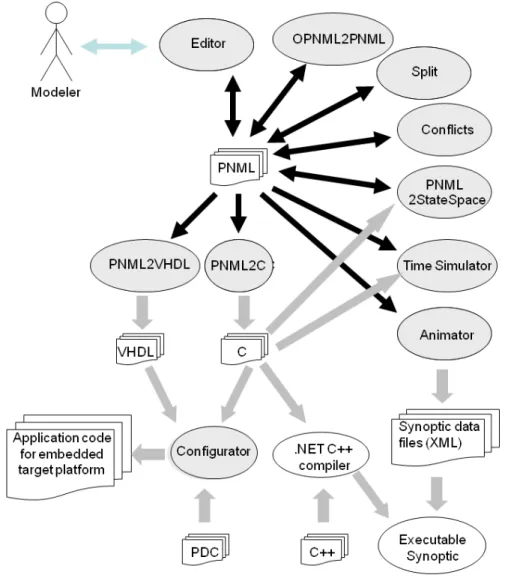
Tools overview

The FORDESIGN project emphasizes the use of tools (2.3): already existent ones and new tools developed within the project. The first group includes UML-based tools, and in particular Use Case diagrams. These will mainly be used in the requirements and analysis phase. The second group, encompasses the development of several interrelated tools which can be classified in the following four basic groups:

1. Modeling; 2. Simulation; 3. Verification; 4. Synthesis.

The Modeling group includes:

• The Graphical Editor - includes support for bottom-up and top-down model construction and animation capabilities [GBCN07];

• Conflict resolution - supported by the generation and recommendation of specific arbiters to handle structural or effective conflicts;

• OPNML2PNML - for model composition [BG04b];

• Split tool - to decompose PNML models into a set of concurrent sub-models (obtained as a contribution of the works supporting this thesis). Within the Simulation group the following tools were considered:

(52)

• Animator - allowing the automatic generation of an animated synoptic based on the association of the characteristics of an IOPT model with specific characteristics of the graphical user interface through a set of dedicated rules [LG08];

The Verification group includes:

• PNML2StateSpace - a state-space generator and analyzer that uses generated C-code;

The Synthesis group is composed by the following:

• PNML2C - translator from PNML to C,

• PNML2VHDL - translator from PNML to VHDL [GCBL07].

• Configurators - to adapt the generated code to the deployment platform [CGB+_{08, OCG09].}

The main rationale for having a relatively large number of tools is to increase flexibility through modularity, much like the philosophy of the well-known

UNIX operating system. In particular, this approach eases model inter-change with existent tools (available from the community); especially UML based tools, verification tools and tools for automatic graph layout.

Fig. 2.3 shows the interdependencies and communication between the dif-ferent foreseen components. Tools are represented as ovals, files as rectangles and information flow as arrows.

The graphical editor is the central tool. It generates PNML and OPNML (Operational PNML) specifications, which are used by most of the other tools. The editor serves as an interface to several tools without a graphical user interface. Through the graphical editor, the modeler will be able to execute the following tasks:

1. Reading and writing of PNML based specifications [SC05, BCvH+_03]; 2. Creation of PNML and OPNML models[BG04b];

(53)

Figure 2.3: The development environment architecture; tool overview.

5. Code generation, for implementation, simulation and verification - a common code base will be used for all three tasks;

6. State-space exploration.

(54)

by optimized memory consumption based on upper bounds for place mark-ings, obtained through associated state space construction. This code can be executed on multiple platforms where the language C is available. Yet, the main focus will be reconfigurable computing platforms, namely FPGAs. Also, the solutions are completely compliant with SoC design. The configu-rator tool allows the specification of several details allowing a code generation optimized for the given platform.

Beyond the above presented classification, the developed tools can be grouped into three main groups:

• First group: Modeling, simulation and verification activities, focusing on modeling with IOPT nets and associated PNML representations; the PNML representations have the central role for this set of tools.

• Second group: Design automation environment, built around the “Con-figurator” tool, addressing the configuration of a specific embedded system, and producing application code to be deployed into a specific embedded target platform.

• Third group: Design automation environment, built around the “Ani-mator” tool, addressing the configuration and automatic code genera-tion for an animated synoptic to be executed under Windows OS PC platform.

The first group of activities starts with using the graphical editor to produce the system models in PNML format. The editor supports animated simulation for the model execution (from the point of view of the autonomous part of the IOPT model) and invokes external applications to perform specific operations, namely the OPNML2PNML tool and the Split tool. The former allows the composition of nets using the net addition operation. The later allows the specification of a cutting set to decompose the model into a set of concurrent sub-models [CG07b, CG07c, CG09]. These concurrent models can be seen as components to be further mapped into software or hardware platforms. For that purpose, translators to C and VHDL are available. It is important to note that the generated C code can be used for several goals, namely final execution, but also for simulation and verification activities.

(55)

of possible mappings of the components into specific implementation plat-forms considering different types of support for inter-component communi-cation. Currently, a small set of platforms is being considered, including Xilinx Spartan-3 FPGA, Xilinx Virtex-II Pro FPGA, and Microchip PIC 18F4620 microcontroller, as well as the MicroBlaze microprocessor IP for Xilinx FPGAs.

The third group of activities addresses the generation of synoptic applica-tions to be executed under Windows OS PC platforms and takes advantage of the association of the IOPT model characteristics and graphical charac-teristics of the synoptic. As a result, an autonomous application is generated allowing the interaction with a simulator and receiving visual feedback from the net model status.

(56)

(57)

Chapter 3 Petri Nets

Summary

This chapter presents an introduction to Petri nets, start-ing with basic definitions followed by a characterisation of the nets as autonomous and non-autonomous. Then the non-autonomous IOPT Petri net class is presented. A brief dis-cussion about Petri net model decomposition and the commu-nication between sub-models is presented.

3.1 Introduction

Petri nets were invented by Carl Adam Petri (12 July 1926 - 2 July 2010) - at the age of 13 (in 1939) - for the purpose of describing chemical processes. He documented his invention in 1962 as part of his dissertation,Kommunikation mit Automaten (communication with automata). Of course, it was not Carl Adam Petri who coined the termPetri net; other scientists later referred to several classes of nets as Petri nets. Most of the authors when proposing a new definition of Petri net, do not introduce something completely new. They base their work on the concepts defined by Petri and add some extension or new features of the net, depending on the purpose of the net which they define.

An extensive introduction to Petri nets is not provided here, but in the following subsections, basic definitions and some general characteristics of the nets are given, complemented with some specific classes which are of special interest for this work.

3.2 Basic Definitions

The following definitions of a net are common to all classes of Petri nets; they have been chosen from [Rei98]. Each definition follows the same structure: two different components representing the “passive” and “active” aspects of the system, which are combined by an abstract relation, always connecting elements ofdifferent sources.

Definition 1. (from [Rei98]) Let P and T be two disjoint sets, and let F ⊆

(P "T)S

(T "P). Then N = (P,T,F) is called a net.

Where P,T, and F are called places, transitions, and arcs, respectively. F is sometimes referred to as the flow relation of the net. Places represent the “passive” elements and transitions the “active” elements.

For graphical representation of a net, we use circles for places, boxes or thin rectangles for transitions and arrows for arcs.

Definition 2. (Adapted from [Rei98]) Let N = (P,T,F) be a net.

• N.P, N.T and N.F denote P,T and F, respectively. By abuse of nota-tion, N often stands for the set PS

(59)

3.2. Basic Definitions

Figure 3.1: Isolated (a), Connected (b) and Strongly connected (c) nets.

• As usual, F−1_{, F}+_{, and} _F∗

denote the inverse relation, the transitive closure, and the reflective and transitive closure of F, respectively, i.e., aF−1_b _{iff bFa, a} _F+_b _iff _{aF c}

1F c2...cnF b for some c1, ..., cn ∈ N and

aF∗

b iff a F+_b _{or a = b. For} _a_∈_N_{, let} _F₍_a_{) =} _{_b_|_{aF b}_}_.

• Whenever F can be assumed from the context, for a ∈ N we write

•a instead F−1₍_a₎ _and _a_• _{instead F(a). This notation is translated to}

subsets A ⊆ N by •A = S

a∈A•a and A• =

S

a∈Aa•. •A and A•

are called the pre-set (containing the pre-elements) and the post-set

(containing the post-elements) of A.

Definition 3. (Adapted from [Rei98]) Let N be a net.

• x∈N is isolated iff •xS

x•=∅.

• N is connected iff for all x, y ∈N :x(F S

F−1₎∗ y.

• N is strongly connected iff for all x, y ∈N :x(F∗

)y.

Figure 3.1 illustrates each of the listed net types.

(60)

the concrete execution semantic can be slightly different, depending on the class of the net.

Two transitions are in conflict when both have the same place as an input node and the firing of one of the transitions disables the other one from firing. As was mentioned before, there are many classes of Petri nets. In [Gom97], they are organized in two groups; autonomous and non-autonomous.

3.3 Autonomous Petri Nets

As the name suggests, autonomous nets are nets where the dynamics do not depend on external conditions but only on the graph dependency; in other words, the execution of the net depends only on the state of the net, which means on the marking of the net. The firing rule is the same as presented before.

The classes which are considered within this group can be subdivided into the following reference levels:

• The first level includes classes where the places may contain zero or one tokens, and the tokens have no associated structure; places represent conditions.

• The second level includes classes where the places may contain zero or several tokens; tokens have no associated structure; places can be seen as containers.

• The third level includes classes where the places may contain tokens with associated structure, which means that they are different from each other. These Petri net classes are usually called high-level Petri nets, as opposed to the classes associated with the previous categories, which are called low-level Petri nets.

(61)

3.4. Non-autonomous Petri Nets

As our objective is to use Petri nets for embedded systems modeling, namely for system behavior modeling, the autonomous nets class which suits best is the place-transition Petri net, which is normally used for automation control modeling.

Definition 4. (Adapted from [Mur89]) A Place/Transition Petri net (P/T net) is defined by a tuple N = (P, T, F, W) where

• P is a finite set of places;

• T is a finite set of transitions — P S

T =∅;

• F is a flow relation F ⊆(P ×T)∪(T ×P) for the set of arcs;

• W is a weight function, W :F →N+_.

3.4 Non-autonomous Petri Nets

(62)

3.4.1 Input-Output Place-Transition Petri net

The IOPT Petri net class is an extension of the class of place-transition Petri nets (e.g. [Rei85]) which allows the interaction between the net that models a controller and the environment. From the net model point of view, and thus from the modeler point of view, the environment is seen as a set of input and output events and signals. These impose some restrictions upon the net model behavior. Hence, the net becomes non-autonomous, in the sense of the interpreted and synchronized nets of David and Alla, and Silva [DA92, Sil85]. Several other works propose some kind of non-autonomous extensions to Petri nets with special attention to factory automation applications, e.g. [VZJ94, FM00, HL00].

A preliminary version of theInput-Output Place-Transition Petri net was proposed in [PBG05] and was calledInput Output Petri Net. It included the communication with the environment through input and output signals. In [GBCN07] an updated version of the IOPT Petri net class was presented. The following characteristics were added to the definition of the IOPT Petri net with respect to Place-Transition nets:

1. Priorities in transitions; 2. A bound attribute for places;

3. Input events (defined using an edge level on signals); 4. Two types for input and output signal values;

5. An explicit specification for sets of conflicting transitions (conflict sets - ConfS);

6. An explicit specification for sets of synchronous transitions (synchronous sets - SS);

7. Test arcs.

(63)

3.4. Non-autonomous Petri Nets

The goal associated with the bound attribute for places is to feed an automatic code generation tool with relevant information for implementation, giving specific hints about needed resources to support place implementation (it does not stand for the common maximum capacity semantics). In fact, it is only filled with the maximum reachable marking after the verification of properties by the PNML2StateSpace tool, which initially runs without defined bound attributes. The objective is to allow memory consumption optimization, in the code generation phase. For this reason, it does not affect the net execution or the model behavior.

The edge level for events has the expected semantics: it specifies which variation of an input signal is considered as relevant. We also allow the modeler to distinguish between two types of signal values: Integer ranges or Boolean values.

Finally, the model representation can also encompass one or more sets of conflicting transitions (the conflict set - ConfS), as well as synchronous transitions. The latter have “fusion semantics”, which means that all the transitions in the set behave as a single one with the input and output arcs of all the set transitions. Hence, these sets can be seen as transition fusion sets.

Within the scope of embedded systems design, the IOPT Petri net is used for modeling the control part of the system. The controller can be characterized by two main components:

1. Description of the physical interaction with the controlled system (the interface of the controller);

2. Description of the behavioral model, which is expressed through a IOPT model.

The controller interface

As already stated, from the net modeler point of view, the controller is a set of active input and output signals and events.

Definition 5(System interface). (from [PBG05]) The interface of controlled system with an IOPT net is a tuple ICS = (IS, IE, OS, OE) satisfying the following requirements:

PETRI NET MODEL DECOMPOSITION - A Model Based Approach Supporting Distributed Execution -

Anik´

o Katalin Horv´

ath da Costa

PETRI NET MODEL

DECOMPOSITION

- A Model Based Approach Supporting

Distributed Execution

-Disserta¸c˜ao apresentada para obten¸c˜ao do Grau de Doutor em

Engenharia Electrot´ecnica, Especialidade de Sistemas Digitais,

pela Universidade Nova de Lisboa, Faculdade de Ciˆencias e

Tecnologia

Acknowledgments

Abstract

Resumo

Contents

I

Background

1

II

Contribution

55

List of Figures

Part I

Chapter 1

Introduction

Contents

1.1

Embedded Systems

1.2

Motivation

N

1.3

Problem Statement

1.4

Objectives

1.5

Contribution

1.6

Structure of the Dissertation

Chapter 2

Related Methodologies

Overview

Contents

2.1

Models of Computation Used in

Embed-ded System Development

2.2

Embedded Systems Development

Frame-work Evolution

2.3

Model Based Development

2.3.1

Model driven architecture

2.3.2

FORDESIGN development flow

Chapter 3

Petri Nets

Contents

3.1

Introduction

3.2

Basic Definitions

3.3

Autonomous Petri Nets

3.4

Non-autonomous Petri Nets

3.4.1

Input-Output Place-Transition Petri net

_N