Todos os direitos reservados.
É proibida a reprodução parcial ou integral do conteúdo
deste documento por qualquer meio de distribuição, digital ou
impresso, sem a expressa autorização do
REAP ou de seu autor.
(Mis)Allocation Effects of an Overpaid Public
Sector
Tiago Cavalcanti
Marcelo Rodrigues dos Santos
(Mis)Allocation Effects of an Overpaid Public
Sector
Tiago Cavalcanti
Marcelo Rodrigues dos Santos
Tiago Cavalcanti
University of Cambridge and Insper
Marcelo Rodrigues dos Santos Insper
(Mis)Allocation Effects of an Overpaid Public
Sector
∗
Tiago Cavalcanti
University of Cambridge and Insper
Marcelo Rodrigues dos Santos
Insper
Abstract
In an economy in which the public sector is productive and factor inputs are rewarded according to their marginal productivity in both the public and the pri-vate sectors, the presence of a large government does not generate necessarily any allocation problem. When the provision of public infrastructure is below its opti-mal scale, then an increase in the size of the government can lead to an increase in total factor productivity (TFP). There is, however, a large body of evidence show-ing that for many countries the structure of wages and pensions and the labor law legislation are different for public and private employees. Such differences affect the occupational decision of agents and might generate some type of mis-allocation in the economy. We develop an equilibrium model with endogenous occupational choice, heterogeneous agents and imperfect enforcement to study the implications of an overpaid public sector. The model is estimated to be con-sistent with micro and macro evidence for Brazil and our counterfactual exercises show that public-private earnings premium can generate important allocation ef-fects and sizeable productivity losses.
Keywords: Public-Private earnings premium; misallocation; and
develop-ment. J.E.L. codes: E6; H3; J2; O1.
∗We have benefited from discussions and conversations with Pedro Amaral, Tiago Berriel, Marco
“Programmers and media industry workers had the highest percentage of self-identifieddiaosi, but only fewer than 10 percent of civil servants self-identified asdiaosi.” Tea Leaf Nation,
June 2013.1
“There are many ways of striking it rich in Brazil, but one strategy may come as a particular surprise in today’s economic climate: securing a government job.” The New York Times,
February 2013.2
“Shaadi.com reported a 30 per cent shift away from IT grooms towards other industries, par-ticularly civil servants and managers at state-owned companies who have higher job security and recently were awarded a large pay rise by the government... Top of the scale are civil servants, those from the ultra-elite Indian Administrative Service and Indian Police Service.”
Financial Times, April 2009.3
1
Introduction
As the anecdotal evidence above (as well as the empirical facts provided in Section 2) suggests a career in the civil service seems to be an attractive profession for many individuals in different societies. Such a career might be associated with a good pay, job stability, and in supplying essential goods and services, such as the rule of law and public infrastructure, for the functioning of any society with direct influence not only in economic outcomes but also in the quality of life of individuals. In many countries a large proportion of the labor force works in the public sector and a large share of output is produced by the government. TheOECD(2011) report,Government at a Glance, shows that there are also important cross-country differences on the share
of the labor force working for government entities, organizations and corporations and on the size of the government. For instance, in 2008 governments in Norway
1Diaosi is a Chinese expression to describe a poor, young and unattractive person in China who
cannot afford to buy a house and is unlikely to marry.The Economist(2014) has also feature a piece on the topic showing that Chinese workers who least identified themselves asDioasiwere civil servants.
2This piece of theThe New York Times(2013) shows anecdotal evidence on how several public
em-ployees have exceeded constitutional limits on their pay, which is roughly US$ 13,000.00. For instance, a clerk at a court in Brazil’s capital, Brasília, was making more than the chief justice of the nation’s Supreme Court. Other examples are of an auditor in Minas Gerais state who earned US$81,000 in one month and a librarian who got US$24,000 per month.
3In this report, theFinancial Times(2009) shows that in the marriage market in India public servant
and Denmark employed about 30 percent of the labor force, while in Korea only 5.7 percent of the labor force was employed in the public sector.
In an economy in which the public sector is productive and factor inputs are paid according to their marginal productivity in both the public and the private sectors, the presence of a large government does not generate necessarily any allocation prob-lem. A larger government can on the contrary increase total factor productivity (TFP) if the provision of public infrastructure is below the optimal scale. There is, however, a large body of evidence showing that for many countries the structure of wages and pensions and the labor law legislation are completely different for public and private employees. Section 2 summarizes the empirical evidence on the public-private in-stitutional and earnings gap. In general, the evidence suggests that, controlling for individual characteristics, public employees are on average better paid, have a more protected job and higher pension than private workers. In a recent work, Depalo, Giordano, and Papapetrou(2013), for example, show that for ten euro area countries wages are on average higher for public than private workers and for some coun-tries such as Greece, Ireland, Italy, Spain and Portugal there is a large fraction of this public-private wage gap that is unexplained by workers’ characteristics. For instance, the raw average wage gap between public and private employees is 43 (36) percent in Portugal (Spain) and about 1/2 (2/3) of this gap is not explained by differences in ed-ucation, experience and other observable characteristics. Could differences in labor compensation (e.g. wages and pensions) and labor legislation (e.g. job security) be-tween private and public workers affect individuals’ occupational choice, investment and generate important loss in aggregate productivity of an economy? This paper addresses this question.
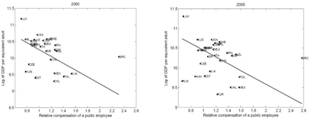
Figure1(see also Table7in AppendixA) presents the relationship between com-pensation of a public employee relative to the income per worker of a country ver-sus the logarithm of the level of output per adult for selected countries in 2000 (left graph) and 2009 (right graph). The best linear fit is shown by a solid line in each graph. Although the correlation in this figure does not imply a causal effect and we do not intend to imply that, we can observe that there is a negative relationship be-tween the relative compensation of a public employee and the level of output per equivalent adult in a sample of basically OECD countries.4Therefore, the cross
coun-4The pooled regression with year fixed effects yields even stronger and more precise correlation.
Figure 1:Relative compensation of a public employee and GDP per adult.Left graph:Data for 2000. Right graph: Data for 2009. Source: Government at a glance, OECD (2011) and Penn World Tables,
Heston, Summers, and Aten(2012). We construct the relative compensation of a public employee by dividing the total compensation of general government employees as a share of GDP by employment in general government and public corporations as a share of the labor force.
try correlation suggests a negative relationship between how public employees are compensated and the level of per capita income. In addition, there is no correlation between the level of output per adult and the share of the labor force in the public sec-tor and the level of output and total compensation of general government employees as a share of GDP.5 The only negative correlation is on the relative compensation
of a public employee and the output per adult person. We provide a framework to understand why a relative overpaid public employee might lead to misallocation of resources and a decrease in overall productivity. Our analysis is both qualitative and quantitative.
Differences in earnings, compensation and labor legislations between public and private workers affect the occupational decision of agents and consequently gener-ate some type of misallocation in the economy. The public sector might attract high productive and risk averse agents looking for a more stable and higher paid job, cre-ating a public sector job queue and crowding out private sector employment and entrepreneurship. This can lead to a negative effect on the average labor productiv-ity of workers in the private sector and it can also decrease the mass and the qualproductiv-ity of entrepreneurs. Therefore, countries might be able to increase their short-run and long-run (if human capital accumulation depends on occupational choices)
produc-5See the last column of Table 7. This is interesting given that there is a positive correlation
tivity by decreasing the public earnings premium and by reforming their labor law legislations. This might be particularly important in countries with inefficient and oversized public sectors. In addition, since fiscal consolidation has recently become one of the main issues in the public policy agenda in most developed countries, the pressure for governments to restructure wages and pensions has increased. This pa-per provides an analysis about the misallocation effects of a generous civil servant compensation and the potential output effects of government reforms to change the pension and wage scheme of public employees.
In order to guide our assessment, we construct an equilibrium model with en-dogenous occupational choice. Firstly, we fix ideas in Section 3 by presenting the static version of the model and deriving some analytical results. Although the static model is a useful device to understand the mechanisms of how the public sector earn-ings premium affects productivity, it is not an appropriate framework for quantita-tive analysis since investment decisions can depend on occupational choice and vice-versa. Then in Section4we consider an overlapping generations economy in which agents live for a realistic number of periods and have preferences over consumption. At each period of time, agents choose whether to work in the public or private sec-tors or to be an entrepreneur, as in theLucas (1978) “span of control” model. When born agents draw from an invariant distribution two types of abilities: An ability to run a business and a labor market productivity. These two abilities evolve over time depending on the agents’ occupational choice in a learning-by-doing and on-the-job training manner.
We calibrate and estimate the model to be consistent with key micro and macro statistics of the Brazilian economy. Brazil is an interesting case since it has a large public-private earnings and compensation premium. See Section2below.6 Then we
perform counterfactual exercises by changing the wage premium in the public sector and by reforming the social security system such that pensions of civil servants are similar to pensions of private workers in the country.7 In the same spirit ofMortensen
6There is also plenty of anecdotal evidence on Brazil’s overpaid public sector. See, for instance,
the New York Times quote above.Financial Times(2014) has also recently featured a piece on Brazil’s public sector:“Looking for a job where you barely have to turn up to work, get paid about 27 times the minimum wage and can retire early on the handsome pension benefits? If the answer is “Yes”, why not try Brazil’s Congress?” Despite being a country with a relative young population and an economy in transition,
Brazil’s government size as a share of income is similar to the OECD average (cf.,OECD,2011).
7We also change the idiosyncratic process of income in order to study aggregate effects of changes
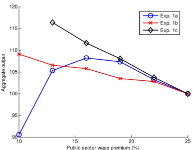
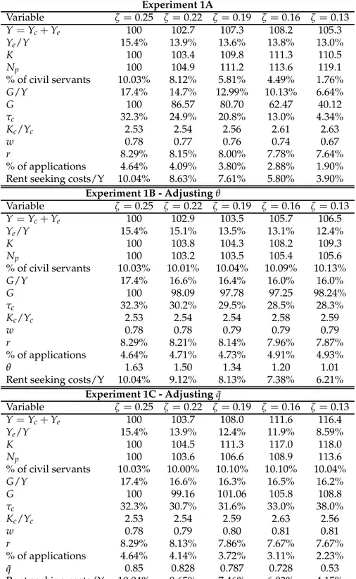
and Pissarides(1994), we keep the share of public employees constant by increasing the probability of a successful public job application (or alternatively by decreasing the cost of applying for a public job). We show that a decrease in the public wage pre-mium from 25 percent to 13 percent can produce a sizeable positive effect on long-run aggregate output (6-16 percent increase) without any significative decrease in public infrastructure. Pension reforms can have similar aggregate effects. There is labor re-allocation and substantial increases in capital accumulation and labor productivity. We believe our results have far reaching implications for policies in countries with a large and inefficient public sector. We also provide a distributive welfare analysis and try to understand the main important channels driving our results.
There are a number of theoretical reasons explaining why earnings differentials between the private and public sector exist. For instance, it might be the case that the bargaining power of public and private workers are different resulting in a wage dif-ferential between the two sectors. The difference in bargaining power by public and private workers might be explained by historical reasons, the type of job associated with public services and/or due to differences in some labor law legislations (e.g., job security, right to strike) between the two sectors. It is not our goal to investigate why such earnings differentials exist and why some legislations protect more public than private employees. We take these wedges in earnings and benefits from the data and calculate the effects of those on investment and the allocation of talents in the economy and therefore on productivity and income levels.
This article is related to a large literature which investigates the underlying causes of low economic development and productivity in some countries. Differences in de-velopment level across countries can be explained by differences in factor accumula-tion and in the efficiency in which these factors are used in producaccumula-tion. The existing literature suggests that both factors accumulation and total factor productivity (TFP) play key role in explaining income levels across countries.8 Human capital and
phys-ical capital accumulation depend on the return of such investments, which in turn depend on incentives and government policies of a society. A standard neoclassical growth model would for instance show that a tax on capital income will decrease in-vestment and long-run income levels (cf.,Lucas,1990). TFP, on the other hand, might
8For a survey of this literature seeCaselli(2005) andHsieh and Klenow(2010).Caselli(2005) very
vary for two main reasons: First, because countries can either use different technolo-gies in the production of goods and services (cf.,Parente and Prescott, 1994) or use similar technologies differently (cf.,Acemoglu and Zilibotti,2001); and secondly be-cause countries do not allocate inputs efficiently. In this second case, factor inputs are misallocated and factor reallocation from less to more productive establishments or jobs could potentially increase output. Hsieh and Klenow(2009), in an influential study, show that there is greater dispersion of productivity in India and China than in the United States and factors reallocation could increase TFP in China by 30-50% and in India by 40-60%. Their goal is to measure the size of misallocation, but they, however, do not explain why it exists. See alsoRestuccia and Rogerson(2008) who show the potential effects of a misallocation in a growth model with heterogenous firms.
The literature on misallocation is growing rapidly in recent years and economists have studied different causes of why inputs of production are not allocated in the most productive manner such that the marginal productivity of input factors are equalized across different firms. Some of the theories to explain such misallocation are based on credit market imperfections and frictions,9taxes and regulations,10trade
policies,11 among others.12 Restuccia and Rogerson (2013) provide an overview of
this literature. Our article differs from this existing literature in an important way as (to our knowledge) none of the articles study the misallocation effects of the public-private earnings and institutional gaps.13
Related to our work isHsieh, Hurst, Jones, and Klenow(2013) who in the same spirit of this paper investigate the aggregate productivity gains in the United States that can be attributed to decreases in labor market discrimination towards
African-9SeeAmaral and Quintin(2010),Antunes, Cavalcanti, and Villamil(2008),Buera and Shin(2013),
Erosa and Hidalgo-Cabrillana(2008),Midrigan and Xu(2013), among others.
10See, for instance,Antunes and Cavalcanti(2007),Guner, Ventura, and Yi(2008), andRestuccia and
Rogerson(2008).
11SeeMelitz(2003).
12Caselli and Gennaioli(2013) study the misallocation effects of dynastic family business. Their main
idea is that if the offspring of the family firm has no managerial talent, then dynastic management is a failure of meritocracy that reduces a firm’s TFP.David, Hopenhayn, and Venkateswaran(2014) study the role of information in misallocation.
13Hörner, Ngai, and Olivetti(2007) study the role of state enterprise in the rise of European
unem-ployment since the late 1970s. Quadrini and Trigari (2007) investigate the role of the public sector on the volatility of employment and output in a match model of the labor market. Related to this,
Americans and women. They show that 15 to 20 percent of growth in output per worker in the United States from 1960 to 2008 can be explained by the decrease in the racial and gender wage gaps. The focus and question of our work are different.14 Song, Storesletten, and Zilibotti (2011) build a model about the Chinese economic transition in which state-owned firms have better access to outside finance than do privately owned firms, even though the latter are more productive. Chinese growth is therefore in part explained by factors reallocation from state-owned to private owned firms and by the reduction in capital misallocation. In our model, the inefficiency is generated by a public sector earnings premium. Therefore, our results are comple-mentary to theirs. Also close to our ideas is a recent contribution byJaimovich and Rud(2014) who study the effects of an oversized and inefficient public sector on eco-nomic performance through an endogenous occupational choice model. Their anal-ysis is qualitative while ours is quantitative. They show, for instance, that when the public sector attracts bureaucrats with low degree of public service motivation, they will use their position to rent seek by employing an excessive number of unskilled workers and leading to an equilibrium with relatively high unskilled wages, which decreases profits and entrepreneurship. Given the focus of their question and in or-der to have an analytical solution, they have to simplify their analysis by for instance considering a static model and assuming exogenous levels of skills (skilled and un-skilled). Our goal is to assess quantitatively the implications of earnings differentials in public and private sectors and therefore we assume endogenous skill formation and a dynamic environment.
The remainder of the paper is organized as follows. The data facts are presented in Section2. Section4presents the model economy. Section5calibrates and estimates model parameters and provides the quantitative analysis to measure the aggregate effects of public-private earnings and institutional gap. Section6contains concluding
14Our environment is dynamic and we consider an entrepreneurial sector with credit frictions. Our
remarks.
2
Data Facts
In this section we document main facts which motivate this study and provide em-pirical support to some of our modelling assumptions and counterfactual exercises.
Before stating the empirical facts related to our interest, we first observe that a large proportion of the labor force works in the public sector and there are impor-tant differences across countries. For instance, in 2008 governments in Scandinavian countries employed almost 30 percent of all workers. This number was 5.7 percent for Korea and about 8.6 percent in Brazil.15 The size of government and consequently the fraction of workers in the public sector vary for several reasons, such as the extension of the franchise to poorer individuals as argued in a seminal paper by Meltzer and Richard(1981), the openness of a country (cf.,Rodrik,1998), or the scope of the pub-lic sector (cf.,Rosen,1996). It is not our goal to discuss what should be the optimal scope of the government or the importance of the government in providing certain public goods and services. We will instead investigate whether or not differences in labor compensation between public and private workers can potentially generate im-portant losses (or gains) in economic efficiency. This motivates the list of the three following factors below.
Fact 1: Public-private wage gap.In most countries there exists a public-private wage
gap. This is not a recent phenomenon. In his empirical narratives, Piketty (2014) shows that in France during the time of Napoleon to World War I there was a small number of very well paid civil servants earning 50-100 times the average wage in the period, such that they could afford to live with “dignity and elegance as the wealth heirs”.Ge and Yang(2014) show that the average real wage in urban China increased by 202% from 1992 to 2007 and the growth was stronger for public employees than for private employees. Using the Brazilian households survey, we show that the condi-tional public sector wage premium ranges from 21 percent to 30 percent, depending on the specification. The empirical evidence suggests that in some countries a large
15Data from the International Labour Organization shows that for 2010 about 10.3 percent of the
fraction of this wage gap is not explained by differences in observed characteristics, such as education and experience. There is a large empirical literature documenting the unexplained wage gap between public and private employees for several coun-tries. Recently,Depalo, Giordano, and Papapetrou(2013) studied the public-private wage gap for ten European countries. For some countries such as Portugal and Spain the raw average wage gap between public and private employees is 43 and 36 per-cent, respectively. In Portugal about half of this gap is not explained by differences in observable characteristics, while in Spain the unexplained public-private wage gap is about 2/3 of the total raw wage gap. A similar pattern is observed in Turkey (cf.,Tansel, 2005), Britain16 (Postel-Vinay and Turon, 2007, cf.,), China (Wang, 2014,
cf.,), and Brazil (cf.,Belluzzo, Anuatti-Neto, and Pazello, 2005). Table 9in Appendix Ashows that the public wage premium varies from 21 to 29 percent depending on the specification and that this does not seem to be driven by unobserved variables. Most studies show that the public-private wage gap decreases for the upper tail of the conditional wage distribution and there is less dispersion in income inequality in the public sector. We show that the dispersion of wages in the public sector in Brazil is similar to the level observed for private sector workers (see Table 8in Ap-pendixA) and the public sector wage premium is quite flat for different quantiles of the conditional wage distribution and it is higher in both tails of the conditional wage distribution including the upper tail (see Figure9in AppendixA).
Fact 2: Public-private pension gap. Not only there exists a public-private wage gap
but in some cases the pension system is also different between private sector and public sector workers. As described in a report from The Economist17 on July 27th 2013, in America most public-sector workers can expect a pension linked to their fi-nal salary. This is not a common practice in the private sector in which only 20 percent of private-sector workers benefit from such a scheme. As The Economist points out when analysing the pension system in the United States, in general in America ’the typical public-sector worker gets a pretty good deal by private-sector standards’.18 A similar
16For Britain, Postel-Vinay and Turon(2007) show that there exists for similar workers a positive
average public premium both in income flows and in the present discounted sum of future income flows. They also find that income inequality is lower and more persistent in the public sector.
17See The Economist, July 27th,Who Pays the Bill?
18Beshears, Choi, Laibson, and Madrian(2011) describe the pension system of the states and the
pattern is also observed in Britain where pensions in the public sector are based on the final-salary (defined-benefit plan) and the pension of private sector workers rely
ondefined-contributionschemes, which is based on how much the employee and
em-ployer contributed and on the return of pension funds.19 Brazil also has a very un-equal pension system, which is divided into two main schemes: a general regime for private sector workers and a special regime for civil servants (cf., Cunha, Ferreira, and dos Santos, 2012). The scheme available to private sector workers consists of a mandatory publicly managed transfer system which covers all private workers up to a ceiling of approximately US$ 1,800. In the public sector, workers can retire with full salary if they are 65 years old and contributed to the pension system for 35 years. Tafner(2011) shows that government expenditures with retirees from the public sec-tor correspond to about 36 percent of the total government expenditures with pension in Brazil, but such expenditures benefit only 7.5 percent of all retirees in the country.20
Fact 3: Public-private institutional gap. The OECD(2011) report shows that many
countries have labor legislation which translates in more secured jobs in the pub-lic than in the private sector. According to Piketty (2014) civil servants in the great depression were immune from the risk of unemployment and some enjoyed an in-crease in their real wages. Clark and Postel-Vinay (2009) construct indicators of the perception of job security for 12 European countries. They find that after controlling for selection into job types, workers feel most secure in permanent public sector jobs and such jobs are perceived to be by and large insulated from labor market fluctua-tions. He, Huang, Liu, and Zhu (2014) provide indirect evidence on job security for China. Using a large-scale reform which decreased job stability in state-owned en-terprises (SOEs) but not for government employees in China in the late 1990s, they show significant evidence of precautionary saving stemming from sudden increases in unemployment risk for SOE workers relative to that for government employees. In Brazil workers in the public sector are guaranteed life tenure after a three-year probation period and since there are no performance evaluation mechanisms in the public sector, rarely an employee is not awarded tenure in the public sector.
Conse-public sector.
19Article byQueisser, Whitehouse, and Whiteford(2008) describes different features of the pension
system in OECD countries.
20The government has changed this for the new public employees. Those who now get a public
quently, tenure in private sector is skewed to the left while in the public sector it is more uniformly distributed.
In the remaining of this article, we will investigate whether or not these institu-tional and earnings gaps generate misallocation and productivity losses in the econ-omy. The economic environment to discipline our analysis is described below.
3
Static Model Intuition
First we present a simplified version of the model to provide some key intuition. The full model is introduced in Section4. For analytical tractability, we consider a static occupational model without capital and close to the environment described by Lu-cas(1978). The economy is inhabited by a continuum of individuals of measure one who live for only one period. Each Individual is endowed with one unit of labor and with entrepreneurial abilityhe, which corresponds to her capacity to employ la-bor, n, in order to produce a single (private) consumption good, yhe. Productivity he follows a continuous cumulative probability distribution denoted by Fe(he). The entrepreneurial production technology is represented by
yhe =Gχh1e−vnv(1−ϕ), v,ϕ∈ (0, 1), χ≥0, (1)
wherevis the span-of-control parameter and 1−ϕdetermines the importance of la-bor in production. G is a public good. FollowingBarro(1990), Gcan be seen as the
stock of public infrastructure such as toll free roads, which is made available to all firms at a zero price. The general idea of includingG as a separate argument in the
production function is that labor n is not a close substitute for public inputs.
En-trepreneurs can operate only one establishment. Letw denotes the wage rate. The
problem of an entrepreneur with managerial abilityhe is to choose labor,n, to maxi-mize:
π(he;w) =max
n≥0 G
χh1−v
e nv(1−ϕ)−wn. (2)
This problem gives labor demand for each entrepreneur:
n(he;w) =
v(1−ϕ)
w G
χ
1−v(11−ϕ)
h
1−v
1−v(1−ϕ)
Then we can also define optimal production and profits of each entrepreneur.
y(he;w) =
"
v(1−ϕ)
w
v(1−ϕ)
Gχ
#1−v(11−ϕ)
h
1−v
1−v(1−ϕ)
e , (4)
π(he;w) = (1−v(1−ϕ))y(he;w). (5)
We assume that the public good,G, is produced by the government using labor,Ng, as the only input such that the production function of the government is given by:
G = AgNg1−α, α ∈ (0, 1), (6)
where Ag >0 is a productivity factor.21
Individuals choose a career in order to maximize income. An individual receives gross incomeπ(he;w)if she becomes an entrepreneur andwif she becomes a worker. They can also be a civil servant. We assume that the public sector wagewg and the
size of the labor force employed in this sector are exogenously determined. In ad-dition, assume that there is a wage premium to work in the public sector, such that civil servants receivewg = (1+ζ)w, whereζ ≥ 0. The public sector is financed by a proportional tax,τc, on consumption.
Let c be consumption of an individual whose preferences are represented by a
function u(c) = c11−−γγ with γ > 0. Individuals maximizes utility subject to the
con-straint that (1+τc)c ≤ y˜, where ˜y corresponds to the income of each household, which depends on the agent career choice.
Lemma 1. For each w>0andζ ≥0, there exists an entrepreneurial ability
¯
he(w;ζ) =
"
(1+ζ)1−v(1−ϕ)w
(v(1−ϕ))v(1−ϕ)(1−v(1−ϕ))1−v(1−ϕ) 1
Gχ
#1−1v
>0, (7)
21Alternatively, we could have assumed that the government produces also the consumption good
with a different technology from the one used by entrepreneurs, such as inSong, Storesletten, and Zilibotti(2011). See alsoWang(2014). For instance, we could have assumed that the entrepreneurial technology is given byyhe = h1
−v
e nv(1−ϕ), while the technology of state-owned enterprises is
repre-sented byyg = AgNgαwithα ∈ (0, 1). This would probably generate stronger effects of an overpaid
public sector on misallocation sinceyhe andygare perfect substitutes in consumption and the
such that for all he ≥ h¯e(w;ζ), thenπ(he;w)≥(1+ζ)w.
Proof. Useπ(he;w)≡(1+ζ)wto find ¯he(w;ζ). Q.E.D.
Notice that ¯he(w;ζ) is continuous and increasing in bothζ and w. This Lemma suggests that individuals withhe ≥h¯e(w;ζ)will choose to become entrepreneurs. In addition, there exists a productivity level ¯hw(w)defined by
0 <h¯w(w) =
¯
he(w;ζ)
(1+ζ)1−v(1−ϕ) ≤h¯e(w;ζ), (8)
which is independent of ζ and is continuous and increasing in w, such that for all he ≤ h¯w(w), then π(he;w) ≤ w. Individuals with entrepreneurial productivityhe ≤ ¯
hw(w)will not choose to be entrepreneurs.
In order to define the agents who become civil servants notice that all individuals with he < h¯e(w;ζ) would like to work in the public sector. But assume that only a fractionφg ∈ (0, 1)can become a public employee and let this be determined exoge-nously in the model. There are several possible cases in which we could select civil servants, but consider two polar examples: (i) in the first case, only individuals with productivityhe ∈ [0, ¯hg]become civil servants, such thatFe(h¯g) = φg. Then, in order to have production of goods in equilibrium, it must be the case that ¯hg <h¯w(w). Con-sequently, all individuals with he ≥ h¯w(w) are entrepreneurs,22 while private sector workers are those individuals with entrepreneurial productivityhe ∈ [hg, ¯hw(w)]. In this case, both ¯hgand ¯hw(w)are independent of ζ. Then changes in the public sector wage premium,ζ, would not affect occupational choice, labor demand and therefore misallocation and aggregate output in equilibrium.23 A second more interesting case
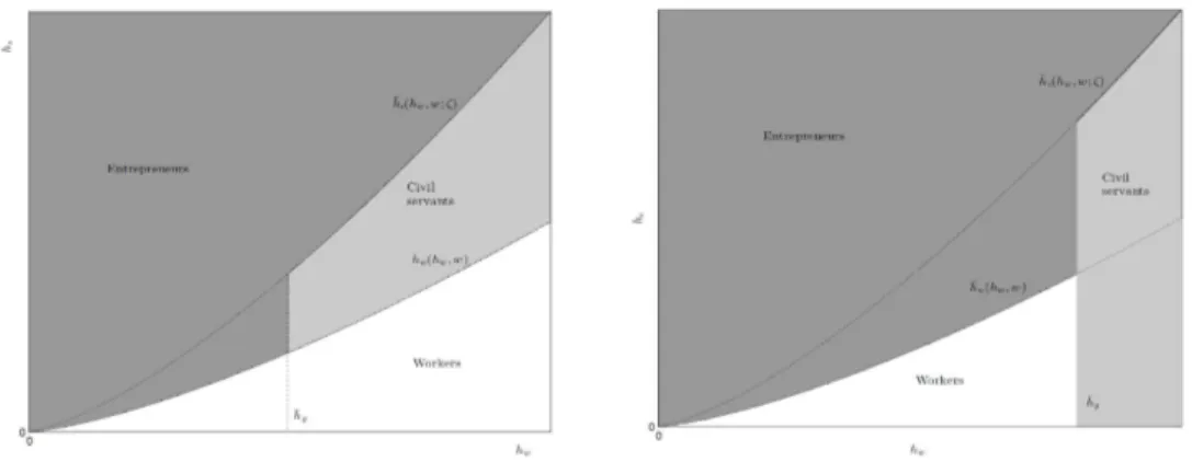
is the one that public employees are defined by individuals withhe ∈ [h¯g, ¯he(w;ζ)), such thatFe(h¯e(w;ζ))−Fe(h¯g) =φg. Sinceφgis held constant, it implies that ¯hg(w;ζ) will be a continuous and increasing function of w and ζ. Figure 2 presents a line which describes the occupational choice for this example, which varies with the size of the public sector. In the left graph, the size of the public sector is not too large and this implies that ¯hg(w;ζ) > h¯w(w), while the right graph shows the case in which ¯
hg(w;ζ) <h¯w(w).
Figure 2: Occupational choice. Left graph: Not too large public sector and employee selection in this
sector depends positively onhe.Right graph:Large public sector and employee selection in this sector
depends positively onhe.
In equilibrium the labor excess demand,LED(w;ζ), is:
LED=
ˆ ∞
¯
he(w;ζ)
n(he;w)dFe(he) +
ˆ max{h¯g(w;ζ),¯hw(w)}
¯
hw(w)
n(he;w)dFe(he)−
ˆ min{h¯g(w;ζ),¯hw(w)}
0 dFe(he),
and the following result can be demonstrated.
Proposition 1. Let public employees be those individuals with entrepreneurial productivity he ∈[h¯g(w;ζ), ¯he(w;ζ)]withh¯g(w;ζ)>0and assume that the government keeps the share
of public employees constant. Then there exists a unique wage rate w(ζ), which clear the labor market. In addition, w(ζ)is decreasing inζ.
Proof. The labor demand function n(he;w)is continuous inwand since productivity levels ¯he(w;ζ), and ¯hw(w)vary smoothly withw, then the labor excess demand func-tion LED(w;ζ)is also continuous in w. In addition,n(he;w)is strictly decreasing in
w, while ¯he(w;ζ)and ¯hw(w)are strictly increasing inw,24which imply thatLED(w;ζ) is strictly decreasing inw. Asw→0, then ¯he(w;ζ)and ¯hw(w)go to zero and no agent wishes to become a worker. It follows that LED(w;ζ) > 0. When wincreases
suffi-ciently, LED(w;ζ) < 0, since all agents wish to become workers (or civil servants).
Therefore, by continuity of LED(w;ζ), there must be an unique 0 < w(ζ) < ∞such
that LED(w(ζ);ζ) = 0. In addition, using the implicit function theorem it can be
shown thatw′(ζ) <0. Q.E.D.
The last part of Proposition1suggests that the wage rate decreases with a higher public sector wage premium. The reason is that a higher wage premiumζ increases the threshold productivity ¯he(w;ζ) and this decreases the demand for labor for a given wage rate. When ¯hg(w;ζ) < h¯w(w) and the government keeps the share of
withhe∈[h¯w(w), ¯he(w;ζ)].
23The tax rateτ
cwill adjust withζand therefore welfare will change withζ, but aggregate output
remains unchanged for a given share of public sector workersφg.
24If the government keeps the number of public employees constant such that Fe(h¯e(w;ζ))−
public employees constant, then an increase in the public sector wage premium in-creases labor supply and dein-creases the share of entrepreneurs in the economy. These two effects lead to a fall in the equilibrium wage rate. When ¯hg(w;ζ) > h¯w(w), then an increase in ζ decreases the share of entrepreneurs with ability higher that ¯
he(w;ζ), but increases by the same proportion the share of entrepreneurs with he ∈ [h¯w(w), ¯hg(w;ζ)]. However, since labor demand varies positively with abilityhe, we have that total labor demand for a given wage decreases. The supply of labor remains constant. Therefore, the wage rate also falls.
Aggregate output for this economy is represented by:
Y =
ˆ ∞
¯ he(w;ζ)
y(he;w)dFe(he) +
ˆ max{h¯g,¯hw(w)}
¯ hw(w)
y(he;w)dFe(he). (9)
Using (4) into the above equation implies that
Y(ζ) =h(v(1−ϕ))v(1−ϕ)Gχi
1 1−v(1−ϕ)
´
E(w(ζ);ζ)h
1−v
1−v(1−ϕ)
e dFe(he)
w(ζ)
v(1−ϕ) 1−v(1−ϕ)
, (10)
where E(w(ζ);ζ) corresponds to the measure of individuals who are entrepreneurs andG= Agφαg. Notice that this equation implies that
Y(ζ) = A¯(ζ) =∝ ´
E(w(ζ);ζ)h
1−v
1−v(1−ϕ)
e dFe(he)
w(ζ)
v(1−ϕ) 1−v(1−ϕ)
.
There are two opposing effects on productivity of an increase in the public sector wage premium when the government keeps the share of public employees constant. The first one is a selection effect. Either the share of entrepreneurs decreases (when ¯
hg(w;ζ) <h¯w(w)) or the quality of entrepreneurs decreases (when ¯hg(w;ζ)>h¯w(w))
share of public employees is constant and all individuals have the same productivity as workers.
An extension of this simple framework is to introduce heterogeneity in labor pro-ductivity. For instance, in addition to entrepreneurial productivity he, assume that each worker is also characterized by an idiosyncratic labor productivity hw, drawn from a continuous cumulative distributionFw(h−w). Therefore, agents are heteroge-nous in the pair(he,hw). Then the following Lemma can be established.
Lemma 2. For each w>0,ζ ≥0, and hw >0there exists an entrepreneurial ability
¯
he(hw,w;ζ) =
"
(1+ζ)1−v(1−ϕ)wh1−v(1−ϕ) w
(v(1−ϕ))v(1−ϕ)(1−v(1−ϕ))1−v(1−ϕ) 1
Gχ
#1−1v
>0, (11)
such that for all he ≥ h¯e(hw,w;ζ), thenπ(he;w) ≥(1+ζ)whw.
Analogously, for eachhw, we can define the line
0<h¯w(hw,w) =
¯
he(hw,w;ζ)
(1+ζ)1−v(1−ϕ) ≤h¯e(hw,w;ζ), (12)
which is independent ofζand is continuous and increasing inw, such that for allhe ≤ ¯
hw(hw,w), then π(he;w) ≤ whw and individuals with productivity he ≤ h¯w(hw,w) will not choose to be entrepreneurs.
The area above line ¯he(hw,w;ζ) is represented by the dark grey shaded area in Figure 3. Individuals with the combination of (he,hw) that lies above ¯he(hw,w;ζ) become entrepreneurs. Individuals whose productivity pair (he,hw) lies below line ¯
he(hw,w;ζ) would like to become civil servants. However, due to job rationing in the public sector not all individuals become civil servant. There are several possibil-ities. Figure3presents two cases. The left graph of Figure 3shows the case in which selection in public sector jobs depends positively on both labor and entrepreneurial productivity, while the graph on the right presents the case in which selection for public employees are entirely based on productivity as workers. Observe that some individuals with productivity below ¯he(hw,w;ζ) but above ¯hw(hw,w) might become entrepreneurs.
Figure 3:Occupational choice.Left graph:Selection in the public sector depends positively onhwand
he.Right graph:Selection in the public sector depends (positively) only onhw.
there will be changes in the share of entrepreneurs as before, but even when the government keeps the share of the labor force constant in the public sector, public infrastructure might also change due to the selection effect on public sector jobs. This simple framework is based on a static model in which the decision to work in the public sector is exogenous and the pair of productivity(he,hw) does not evolve over time. In addition, there is no wealth dynamics, income risks, capital in production and credit market frictions, which can also affect occupational choices and therefore the misallocation effects of an overpaid public sector. Consequently, this static model provides a useful device to understand the mechanism of how a public sector earn-ings premium might affect productivity, but it is certainly a limited environment for quantitative analysis. We therefore present next the full model in which we will base our quantitative results.
4
The Environment
4.1
Demography, preferences and Career choices
Time is discrete and the economy has an infinite horizon. The economy is populated by a continuum of individuals of mass one who may live at mostT periods. In each
time period, a new generation is born with probability one. These individuals sur-vive for a finite number of periodsT, which is deterministic. The age profile of the
and satisfies ∑T
t=1µt = 1, such that the implicit survival rate is ϑt =
µt
µt−1. This
sur-vival probability implies that a fraction of the population leaves accidental bequests, which, for simplicity, are assumed to be distributed to all surviving individuals in a lump-sum basis. In order to simplify notation we omit the time subscript.
They derive utility from consumption, ct, and when not retired individuals are endowed with one unit of time in each period. Preferences over random paths for consumption over the life cycle are represented by:
Et=1
"
T
∑
t=1βt−1
t
∏
j=1ϑku(ct)
#
, (13)
where β is the subjective discount factor, and E is the expectations operator
condi-tional on information at birth. The period utility is assumed to take the form of a power utility function:
u(ct) = ct 1−γ
1−γ, (14)
whereγdenotes the risk aversion parameter or the inverse of the intertemporal elas-ticity of substitution.
In each period, agents decide whether to run an entrepreneurial activity, e, or to
supply their time endowment to the labor market. In the latter case, they can choose to work either in the private sector, wk, or as a civil servant, cs. At a certain age Tr, agents retire and receive social security payments at an exogenously specified re-placement rate of current average wages. The social security regime in the public sec-tor is different from the one in the private secsec-tor. We capture this feature by allowing the replacement rate to differ under the two regimes. Letdm,tform ∈ {cs,wk,e,rg,rp} denote an individual’s occupation, where drg,t denotes and individual who retired from the public sector anddrp,t denotes an individual who retired from the private sector. These occupational statuses are mutually exclusive, which means that, for instance, ifdcs,t =1 thendm,t =0 for allm 6=cs.
4.2
Private sector technology
each business activity is related to one specific manager.25 Households engage in
en-trepreneurial activities in this sector. The second (Corporate sector) one is dominated
by large impersonality units of production (large firms). The main features that dif-ferentiate a small business from a big corporation are the uninsurable entrepreneurial risk and the strictness of the financial constraints. TheCorporate sector does not face
the same incentive problems and risks of the sector intensive in management skills and its presence is important for the quantitative analysis since in the data not all production is generated by business activities associated to one household.
Noncorporate sector. Total production in the noncorporate sector is generated by
the aggregation of all production technologies run by households engaging in en-trepreneurial activities. Each technology comprises a manager with enen-trepreneurial ability, he, which corresponds to her capacity to employ labor, n, and capital, k, to produce a single (private) consumption good, yhe. Subsection 4.4 describes how he evolves over time. The entrepreneurial production technology is represented by
yhe =zGχh1e−vf(k,n)v =zGχhe1−v(kϕn1−ϕ)v, v,ϕ∈ (0, 1), χ ≥0. (15)
Variablezis a random shock. We assume a very parsimonious representation for z, such that in every period with probability ∆, the same technology is available for
the entrepreneur and z = 1. However, with probability 1−∆, z = 0, there is no
production and the individual becomes a worker. Production takes place after the realization ofz. This captures uncertainty related to the entrepreneurial activity.
Managers can operate only one establishment. Letwdenotes the wage rate. The
problem of an entrepreneur agedtwith managerial abilityhe,t and capital stock kt is to choose labor,nt, to maximize:26
πt(he,t;kt) =max
nt≥0
Gχh1e,−tvf(kt,nt)v−wnt. (16)
The choice of capital input is a bit more complicated, since capital has to be paid in advance and there is a commitment problem. Entrepreneurs can finance their
busi-25See alsoWynne(2005).
26Variable zis realized before production takes place. Therefore, it does not appear in the static
problem of the entrepreneur because implicitly we are assuming that when there is production then
ness by using their net wealth or by borrowing from financial intermediaries. Denote byatan agent’s wealth and byrthe endogenous interest rate. Individuals have access to competitive financial intermediaries, who receive deposits and rent capitalkat rate Rto entrepreneurs. The zero-profit condition of the intermediaries impliesR =r+δ, wherer is the deposit and lending rate andδ is the depreciation rate. Borrowing by entrepreneurs is limited by imperfect enforceability of contracts. We assume that, af-ter production has taken place, entrepreneurs may renege on the financial contract. In such case, entrepreneurs can keep fraction 1−φof the underpreciated capital and the revenue net of labor payments, but they lose their financial assets deposited with the financial intermediary,at. Thus, the entrepreneurs’ incentive compatibility constraint can be written as follows:
πt(he,t;kt)−Rkt ≥(1−φ)[πt(he,t;kt) + (1−δ)kt]−(1+r)at. (17)
The incentive compatible constraint (17) guarantees that ex-ante repayment promises are honoured, such that there is no default in equilibrium. Given factor priceswand R, final profits of an entrepreneur agedtis given by:
Πt(at,he,t) =max kt≥0
πt(he,t;kt)−Rkt, (18)
subject to (17).
Corporate sector. Firms in the corporate sector produce the consumption good through
a standard constant returns to scale production function:
Yc =GχKαcNc1−α, α ∈ (0, 1). (19)
profits. The first-order conditions of a representative corporate firm are given by:
r =αGχ
Kc
Nc
α−1
−δ, (20)
w= (1−α)Gχ
Kc
Nc
α
. (21)
4.3
Government sector
We assume that the public good is produced by the government. The public good,G,
is produced using efficient labor units Ng and capitalKg according to the following technology:
G= AgKαgNg1−α, Ag>0. (22)
Public sector capital evolves according to the following law of motion:
Kg,t+1= Ig+ (1−δg)Kg,t, (23)
where public investmentIgis financed through taxes.
There are two different social security regimes: A scheme for private workers and entrepreneurs and a scheme for public workers. The replacement rate for civil servants is different from the one faced by private sector workers. This is consistent with Fact 2 in Section2. Consequently, in the model we have two types of retirees: individuals who retired from the public sector and individuals who retired from the private sector.
In addition, we assume that the government carries out an exogenous flow of expenditure,Cg, which includes other parts of government consumption such as mil-itary expenditure that is deemed to be unproductive in our model. As we show later,
4.4
Households
Human capital accumulation. Individuals are heterogeneous with respect to their
entrepreneurial ability,he, which is the capacity of agents to employ capital and labor more or less productively. Households are also heterogeneous with respect to their efficiency units of labor, hw. We assume that the initial distribution of he follows a log-normal distribution with location parameterµeand scale parameterσe; while the initial distribution of hw follows a log-normal distribution with location parameter
µw and scale parameter σw. Individuals can enhance their future skills by investing in human capital accumulation. The law of motion forhwandhe are given by:
h′w =ξw(hwxw)ψw+ (1−δh)hw, (24)
h′e =ξe(hexe)ψe + (1−δh)he, (25)
where δh is the depreciation rate and (xw,xe) denote investments in working and entrepreneurial ability, respectively. Since human capital investment is intensive in time, we assume that (xw,xe) are denoted in units of time. This corresponds to on-the-job training human capital accumulation. To keep the model tractable, workers are not allowed to invest in their entrepreneurial ability and entrepreneurs are not allowed to invest in their ability as workers.
Budget constraints. In each period of life, and conditional on the career choice,
in-dividuals make decisions about asset accumulation and investments in human cap-ital. Individuals’ labor productivity in the private sector is determined by an age-efficiency index given by hw,texp(st), where st is a random component that evolves according to an AR(1) process given byst =ρst−1+εtwith innovationsεt ∼ N(0,σε2).
Analogously, the evolution of labor productivity in the public sector is represented by
hw,texp(sg,t), where sg,t is an AR(1) process given by sg,t = ρgsg,t−1+εg,t with inno-vations εg,t ∼ N(0,σε2g). This is to be consistent with the fact that labor legislation
We can write individual’s earnings (before taxes) in occupationm∈ {cs,wk,e}as:
˜
ym,t =
(1+ζ)whw,texp(sg,t)(1−xw,t), if civil servant (m=cs);
whw,texp(sp,t)(1−xw,t), if private sector worker (m=wk);
Πt(at,he,t(1−xe,t)), if entrepreneur (m =e).
Parameterζ corresponds to the wage premium that public sector workers receive relative to their counterparts in the private sector. Individuals can resort to self-insurance to protect themselves against the uncertainty on labor income. They can trade an asset subject, which is denoted by at and takes the form of capital. Agents are not allowed to incur debt at any age, so that the amount of assets carried over from aget to t+1 is such that at+1 ≥ 0. Furthermore, given that there is no
altru-istic bequest motive and death is certain at the ageT+1, agents in the end of their life consume all their available resources, that is, aT+1 = 0. At period tthe budget
constraint of an active individual is given by:
(1+τc)cm,t = [1+ (1−τk)r]am,t + (1−τ)y˜m,t−IA,tθ−a′m+tr, (26)
form ∈ {cs,wk,e}. Variable trcorresponds to lump-sum transfers due to accidental
bequests. We assume that (e.g., constitutional rules) the hiring process for civil ser-vants is provided by public competition. Agents in the private sector who want to work in the public sector must take open exams and only those who obtain the best grades on these tests become eligible to fill a pre-determined number of job positions. We assume that the score,qt, of an individual who decides to take one of those exams is a random variable withU[0, 1]. In addition, the cost that an individual who ap-plies for a public sector job faces is captured by the variableθ, and IA,t is an indicator function that takes value 1 if she chooses to apply for a public job and 0 otherwise.
The timeline of events in the public sector recruitment is as follows. An individual who decides to apply for a public sector job at agetfaces the costθintbut will find
out her score at beginning of aget+1. The individual then can only choose to work for the government in the case thatqt+1 ≥q¯, where ¯qis the selection criterion that can
depends on the number of vacancies. We could conditioned the entry to a public sector job by the individual human capital level and ability shock. We use the above approach to simplify the analysis. Also, we view the public sector as a continuous of different jobs which would require different levels of human capital. The fixed lump-sum cost to apply for a public job implies that in equilibrium the decision to apply for a public job will be correlated with individual’s human capital, shocks and assets. In addition, the present approach would in some way understate the effects of an overpaid public sector on misallocation and efficiency.
At ageTr, agents retire and start collecting social security payments at an exoge-nously specified replacement rate of the last period earnings. Consistent with Fact 2 above, there are two main differences in the calculation of retirement benefits in each sector. First, the replacement rate,ηm, in the public sector is higher than in the private sector. Second, benefits in the private sector are capped by a limit denoted by ¯b, while
there is no benefit cap in the public sector. Thus, the budget constraint for retirees can be written as follows:
(1+τc)cm,t = [1+ (1−τk)r]am,t+bm,t−a′m+tr, (27)
wherebm,t denotes the benefits and is given by:
bm,t =
ηrgy˜cs,Tr−1, if retired in the public sector;
ηrpmin{y˜m˜,Tr−1, ¯b}, ˜m ∈ {wk,e}, if retired in the private sector.
Recursive formulation of individuals’ problems. Let Vm,t(ωt) denote the value function of an individual agedt in the occupationm, where ωt = (at,hw,t,he,t,st,zt) is the individual state space. In addition, considering that agents die at age T and
that there is no altruistic link across generations, we have that Vm,T+1(ωT+1) = 0.
recursively represented as follows: 27
Vw,t(ω) = Max a′w≥0,xw≥0,IA,t∈{0,1}
: u(cw)+
βϑt+1
IA,tP(q ≥q¯)Es′maxVcs,t+1(ω′),Vw,t+1(ω′),Ve,t+1(ω′) +
[1−IA,tP(q ≥q¯)]Es′max
Vw,t+1(ω′),Ve,t+1(ω′)
, (28)
subject to (26), whereω′ = (a′,h′w,h′e,s′,z′ =1). Analogously, the recursive problem of individuals who are entrepreneurs can be represented by:
Ve,t(ω) = Max a′
e≥0,xe≥0,IA,t∈{0,1}
: u(ce)+
βϑt+1
IA,tP(q ≥q¯)Es′Ez′maxVcs,t+1(ω′),Vw,t+1(ω′),Ve,t+1(ω′) +
[1−IA,tP(q≥q¯)]Es′Ez′maxVw,t+1(ω′),Ve,t+1(ω′)
, (29)
subject to (26), whereω′ = (a′,h′w,h′e,s′,z′).
Civil servants do not need to apply again for a government job in order to con-tinue working in the public sector. As a consequence, their problem can be written as follows:
Vcs,t(ω) = Max a′cs≥0,xcs≥0
: u(ccs) +βϑt+1Es′maxVcs,t+1(ω′),Vw,t+1(ω′),Ve,t+1(ω′) ,
(30) subject to (26), whereω′ = (a′,h′w,h′e,s′,z′ =1).
Finally, since retires only choose their next period assets, their problem is very straightforward and can be written as follows:
Vm,t(am) = Max a′m≥0
: u(cm) +βϑt+1Vm,t+1(a′m), (31)
subject to (27) form=rg,rp.
27In order to simplify the notation, we have suppressed the subscript for age from both the state and
4.5
Recursive competitive equilibrium
At each point in time, agents differ from one another with respect to agetand to state ωt = (at,hw,t,he,t,st,zt) ∈ Ω. Agents of age tidentified by their individual statesω, are distributed according to a probability measureλt defined on Ω, as follows. Let (Ω,̥(Ω),λt) be a space of probability, where̥(Ω) is the Borel σ-algebra on Ω: for
eachη ⊂̥(Ω),λt(η)denotes the fraction of agents agedtthat are inη.
Given the age tdistribution, λt, Qt(ω,η) induces the age t+1 distribution λt+1
as follows. The functionQt(ω,η)determines the probability of an agent at agetand state ω to transit to the set η at age t+1. Qt(ω,η), in turn, depends on the policy functions in (28), and on the exogenous stochastic process forz. Now, we have all the
tools to characterize the stationary recursive competitive equilibrium. Households’ optimal behavior was previously described in detail above as well as the problem in the corporate sector, non-corporate sector and the government sector. It remains, therefore, to characterize the market equilibrium conditions, the aggregate law of motion, and the government budget constraint. In each period, there are three prices in this economy (w,r,R), but R = r+δ. The equilibrium in the labor and capital markets are defined by:
Kp = TR
∑
t=1 µt ˆ Ωde,t(ω)kt(ω)dλt+Kc = T
∑
t=1 µt ˆ Ωdm,tam,t(ω)dλt,
Np= TR
∑
t=1 µt ˆ Ωde,t(ω)nt(ω)dλt+Nc = TR
∑
t=1 µt ˆ Ωdw,t(ω)hw,t(ω)exp(sp,t)(1−xw,t(ω))dλt,
Ng= TR
∑
t=1 µt ˆ Ωdcs,t(ω)hw,t(ω)exp(sg,t)(1−xw,t(ω))dλt.
The consumption tax rate,τc, is such that it balances the government’s budget,
Cg+Ig+ (1+ζ)wNg+B=τ(wNp+ (1+ζ)wNg+Π) +τkrKp+τcC,
de-notes total benefits. The distribution of accidental bequests is given by:
tr = T
∑
t=1µt
ˆ
Ω
(1−ϑt+1)dm,ta′m,t(ω)dλt.
Finally, given the decision rules of households, λt(ω) satisfies the following law of motion:
λt+1(η) =
ˆ
Ω
Qt(ω,η)dλt ∀η ⊂̥(Ω).
5
Quantitative Analysis
In order to study quantitatively the effects of a generous civil servant compensation and government reforms which would change the pension and wage scheme of pub-lic employees on economic efficiency, we must assign values for model parameters. We proceed by calibrating and estimating parameters such that the model economy matches key micro and macro statistics of the Brazilian economy. Brazil is an interest-ing case since it has a large public-private earninterest-ings premium. The model, however, is sufficiently general to be applied to other countries, such as Spain, Portugal, India, among others. Below is the description of how we set the value of parameters.
5.1
Calibration and estimation
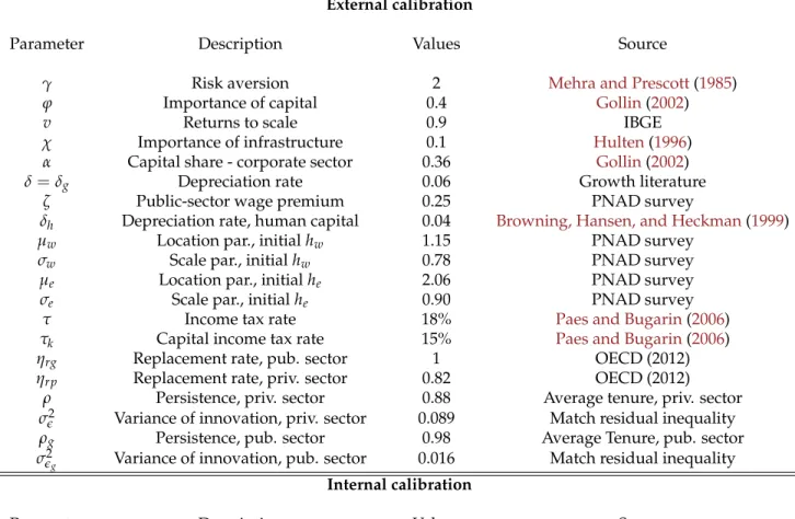
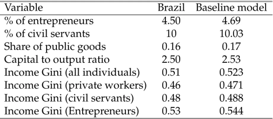
Table 1 lists the value of each parameter for the Brazilian economy and includes a comment on how each was selected.
Model period and age distribution: The model period is one year. We assume that
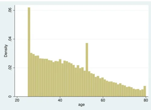
individuals start their lives at the age of 25 and live until the age of 80. Therefore, the extension of individuals’ lifetime in the model is 56 periods (T=56). The age pop-ulation distribution,{µt}Tt=1, is obtained from the 2008 Brazilian households survey
(PNAD). Figure4shows the population distribution by age for 2008.
Utility: There are two parameters related to preferences, (β,γ). The intertemporal discount factor, β, is calibrated such that the capital-to-output ratio is about 2.5.28
28Using theHeston, Summers, and Aten(2012) Penn World Tables 7.1 and the inventory method,
0
.02
.04
.06
Density
20 40 60 80
age
Figure 4: Age population distribution. Source: 2008 PNAD.
The coefficient of relative risk aversion, γ, is set at 2.0, which is consistent with the evidence inMehra and Prescott(1985).
Production technologies: We set ϕ and v so that in the entrepreneurial sector 54%
of income is paid to labor, 36% is paid to remunerate capital, and 10% are profits. Therefore, ϕ = 0.40 and v = 0.90. In the corporate sector, we set α = 0.36. These values are consistent with the numbers provided byGollin (2002). In addition, we assume that the capital stock depreciates at a rate of 6% per year, which is consis-tent to the figures used in the growth and development literature (cf., Parente and Prescott,2000). We also setδg =0.06. According to the Brazilian Institute of Geogra-phy and Statistics (IBGE), the ratio of public goods to output is roughly 16% - using information on production costs. Then, in order to match this ratio we setAg =0.85. To calibrate parameter χ, we rely on estimates provided byHulten(1996) who uses a cross-section of low income countries including Latin American countries and ob-tains a point estimate of 0.1 forχ, which is the value we use. We set the business risk
∆ = 0.04 such that we match the exit rate in Brazil and we calibrate φsuch that the
share of entrepreneurs in the labor force is equal to 4.7. See Table8in AppendixA.
stochas-tic component of individuals labor productivity are: ρ,σε2,ρg,σε2g. For computational
reasons, we use the algorithm described in Tauchen (1986) to approximate these stochastic processes for each sector by a first-order Markov chain with 3 points. Since there is no household panel dataset for Brazil comparable with the Panel Study of In-come Dynamics (PSID) in the United States, we can not obtain direct estimates for the persistence parameters,ρandρg. Thus, what we do is to use information on average tenure in each sector along with data on the distribution of residual wages to calibrate them. In particular, from the Mincerian regressions presented in Table9(columns (6) and (7)), we have that the residual variance for civil servants and private workers are nearly the same: σs2 = σε2
1−ρ = 0.4279 and σs2g = σε2g
1−ρg = 0.4290.
29 We calibrateρ and
ρg in such a way that the average time that individuals take to change position in the grids forsandsgare consistent with the average tenure in each sector, which is about 13 years for public employees and 7 years for private workers. This procedure entails that(ρ,σε2) = (0.88, 0.089)and(ρg,σε2g) = (0.98, 0.016).
30 These figures are consistent
with the fact that public sector wages are more stable and more compressed than in the private sector. This implies that workers facing bad (good) shocks in the pub-lic sector are better-off (worse-off) than their comparable counterparts in the private sector.31
Human capital functions:We calibrate the parameters of the initial skill distribution
of newborn agents,µw and σw for working ability andµe and σe for entrepreneurial ability, to match the wage distribution of workers and entrepreneurs, respectively, at age 25, which is the age individuals are born in the model. The parameters of the human capital functions are calibrated as follows. First, given that the evidence for the human capital depreciation rate ranges from 0.0016 to 0.089, with most of the es-timates concentrated around 0.04 (Browning, Hansen, and Heckman, 1999), we set
29The estimation procedure is presented in AppendixA. 30The associated grids for s
g and s are {−0.3752, 0, 0.3752} and {−0.8955, 0, 0.8955},
respec-tively. In addition, the transition matrix in the public sector is
0.9251 0.0749 0.0000
0.0668 0.8664 0.0668 0.0000 0.0749 0.9251
, while
0.8729 0.1271 0.0000
0.0668 0.8664 0.0668 0.0000 0.1271 0.8729
is the transition matrix in the private sector.
31For the sake of comparison,Kaplan(2012) estimates similar stochastic process for labor
Table 1: Estimation and calibration of model parameters: Brazilian economy
External calibration
Parameter Description Values Source
γ Risk aversion 2 Mehra and Prescott(1985)
ϕ Importance of capital 0.4 Gollin(2002)
v Returns to scale 0.9 IBGE
χ Importance of infrastructure 0.1 Hulten(1996)
α Capital share - corporate sector 0.36 Gollin(2002)
δ=δg Depreciation rate 0.06 Growth literature
ζ Public-sector wage premium 0.25 PNAD survey
δh Depreciation rate, human capital 0.04 Browning, Hansen, and Heckman(1999)
µw Location par., initialhw 1.15 PNAD survey
σw Scale par., initialhw 0.78 PNAD survey
µe Location par., initialhe 2.06 PNAD survey
σe Scale par., initialhe 0.90 PNAD survey
τ Income tax rate 18% Paes and Bugarin(2006)
τk Capital income tax rate 15% Paes and Bugarin(2006)
ηrg Replacement rate, pub. sector 1 OECD (2012)
ηrp Replacement rate, priv. sector 0.82 OECD (2012)
ρ Persistence, priv. sector 0.88 Average tenure, priv. sector
σǫ2 Variance of innovation, priv. sector 0.089 Match residual inequality
ρg Persistence, pub. sector 0.98 Average Tenure, pub. sector
σǫ2g Variance of innovation, pub. sector 0.016 Match residual inequality Internal calibration
Parameter Description Values Source
β Discount factor 0.98 Capital to output ratio, 2.5
φ Enforcement parameter 0.40 Share of entrepreneurs, 4.7%
ξw Human capital productivity 0.14 Life cycle workers’ income
ξe Human capital productivity 0.17 Life cycle entr.’ income
ψw On the job training parameter 0.50 Life cycle workers’ income
ψe On the job training parameter 0.75 Life cycle entr.’ income
∆ Business risk 0.04 exit rate, IBGE
θ Cost of applying for a public job 1.63 Flow of individuals aged 30-34 from private to public jobs ¯
q Government selection criteria 0.84 Share of public servants
τc Consumption tax 0.32 Balance gov. budget constraint
Ag TFP - Government sector 0.85 Share of public goods
¯
b Ceiling for retiree income, priv. sector bmax−cs
bmax
cs =0.16 PNAD survey