Determinants of fiscal budget volatility in old versus new EU member states

(1)

Carlos Pestana Barros & Nicolas Peypoch

A Comparative Analysis of Productivity Change in Italian and Portuguese Airports

WP 006/2007/DE _________________________________________________________

Eugenia-Ramona Mara

Determinants of fiscal budget volatility in old versus new

EU member states

WP 31/2012/DE/UECE _________________________________________________________

De pa rtme nt o f Ec o no mic s

W

ORKING

P

APERS

ISSN Nº 0874-4548

School of Economics and Management

(2)

1

Determinants of fiscal budget volatility in old versus new EU

member states

Eugenia-Ramona Mara1,2

September 2012

Abstract

In this study we perform an analysis of the volatility of the budget deficit for EU countries. We address this issue starting from the new requirements of fiscal discipline imposed by the Treaty on Stability, Coordination and Governance adopted by 25 European Union member states and taking into account the economic crisis impact. The major purpose of this study is to identify the most significant determinants of budget deficit volatility in a comparative study for old EU member states and New Member States (NMS). This study aims to test the impact of macroeconomic variables such as public expenditures, economic growth rate, and unemployment on the budget balance volatility, based on panel data.

The final purpose of the article is to reveal the strategies to stop the immense increase in fiscal deficits and to regain fiscal stability to fulfil the new rules of fiscal governance. We anticipate that the implementation of this new fiscal discipline requires a more efficient public sector for both old and NMS and a reconsideration of state intervention in the economy.

Keywords: budget deficit; fiscal policy; economic growth.

JEL Classification: H62; E62; H3; H61;

1_{Finance Department, Babes-Bolyai University, Faculty of Economics and Business Administration , Cluj-Napoca,}

Teodor Mihali Street, no. 58-60, Romania, , E-mail: ramonanandra@yahoo.com

2_{The research for this article was conducted at UECE, ISEG, UTL, Lisbon. The author thanks}

for helpful comments António Afonso and Juan Carlos Cuestas.

(3)

2

1. Introduction

This paper examines the effects of economic, political and fiscal variables on the budget balance volatility. We begin this analysis with a review of the major empirical and theoretical papers in this area, that explain the methodology used for this study, and also a short descriptive analysis of data.

Moreover, the paper highlights the most important determinants of the budget deficit for the EU countries based on asymmetric analysis between the old and new member states. Based on the empirical findings we try to underline some new trends for the fiscal policy promoted by the EU member states for reducing the level of public debt on the long run and implicitly assuring a better stability for the public finances in the EU.

The new fiscal discipline imposed by this “fiscal compact” is based on stricter surveillance within the euro area, in particular by establishing a "balanced budget rule". We develop this comparative study because we consider relevant the asymmetric conditions for these two groups of countries concerning fiscal policy. The EU new member states are countries with some particularities in their political, institutional and economic context. Our methodology is based on a descriptive analysis of the evolution of the budget deficit and also on and econometric analysis of correlation between budget deficit volatility and other macroeconomic variables like public expenditures, economic growth rate, unemployment, population, and inflation. The study used annual data starting with 1996-2011 based on panel data techniques.

The global financial crisis brought to the forefront the issue of the fiscal deficit and public debt which continued to growing fast in the last five years. This is the result of the fiscal policies promoted by the governments, but also the result of macroeconomic, political and social

circumstances.

In this regard, Cornia & Nelson (2010) mention two main factors which can affect the growth

and volatility of state tax revenue receipts over the business cycle. First, the uniqueness of each

state’s economy ultimately affects its growth and volatility. Second, a state’s choice of taxes, tax

(4)

3

The issue of reducing the fiscal balance deficit and fulfil the requirements imposed by the EU – maximum 3% of GDP (Stability and Growth Pact) for the budget deficit and more recently (through Treaty on Stability, Coordination and Governance - Fiscal Compact) for the annual structural government deficit 0.5% of GDP – becomes an important challenge for all EU members states nowadays. The global financial crisis not only changed the economic and political framework and imposed new fiscal policy measures, but also a new trend for the fiscal policy of the EU member states. Based on these new conditions the member states try to reduce the budget deficit increasing VAT rates and decreasing public expenditure. The huge budget deficits cannot be accepted as a solid ground of economic growth because of the level of public debt, which tends to be an equation without solution for many countries like Greece, Italy, Ireland or Portugal, where the public debt level is more than 100% of GDP.

Considering the requirement of structural government deficits we consider as a possible solution for reducing the public debt or at least maintaining a stable level on the long run – reducing the budget deficit volatility. Some countries try to have a budget surplus for improving the public finance stability, for instance in 2011 – Hungary + 4.3% of GDP, Estonia + 1% of GDP and Sweden +0.3% of GDP, but obviously on the long run the budget surplus is hard to be maintained. A high variation between deficit and surplus of the budget means instability of revenues and unpredicted sources of financing for public expenditures. Based on this, reducing the budget deficit volatility it is a proper solution for assuring the public finance stability in the long run. Breunig and Koski (2011), explain why is so important a lower budget volatility from needs-based perspective, and underline the impact of huge budget volatility on the public expenditures altering the public service financing. The same author defines the budget volatility as variation of budget expenditures over time, but we consider not only the expenditure side, but also the revenue side for computing the volatility.

In this paper we try to isolate what are the major factors that contribute to the volatility of budget deficits increases for the EU countries. Our analysis consider an asymmetric behaviour between the 12 new member states (NMS12)3 and the old member states (EU15) based on the different

3_{The countries are: Estonia, Latvia, Lithuania, Romania, Bulgaria, Poland, Czech Republic, Slovenia, Slovakia,}

(5)

4

degree of development - a higher GDP per capita in the old member states, a higher economic growth rate in the NMS12, and also with different trends of fiscal policy between this two groups of countries. This study tries to test this asymmetry concerning the determinants of budget deficit and fiscal policy between the old member states and the new EU members.

Even if many NMS12 countries have a lower public debt (below 60%) budget deficit volatility represents an important cause of public finances’ instability and for this reason also these countries should act for counteracting this volatility in the long run. If this budget volatility is the result of a boost of economic growth is not seen as a danger, but if it is a consequence of a recession becomes a major issue for the governments. The major characteristics of their fiscal policy are a lower tax burden with proportional income taxation and also a lower level of public expenditures.

On the other hand, the old member states have a higher tax burden with progressive income taxation, a high degree of spending because the welfare state is more developed and also public indebtedness is higher. In this context the budget balance evolution is quite different between these two groups of countries. The major concern of all EU countries remains the public debt and finding solutions for reducing it, and a good start point is reducing the budget balance volatility in the long run. This means stable revenues and expenditures for the government, but how can that be accomplished after five years since the beginning the global financial crisis? Definitely we are referring to a few solutions not just one, and these have to be different between the EU countries. The huge disparities concerning the level of public debt require specific solutions, but all these solutions have the same ground in the end – increasing the efficiency of the public sector. The welfare state has to become more efficient and act like a private welfare state based on efficiency and productivity. In this context our analysis proceeds to identify the macroeconomic determinants of budget volatility and the measure in which they can be changed for reducing this volatility.

(6)

5

2. Literature review

Following the previous studies on this subject, we can synthesize a few research directions, for instance:

- studies focused on the causes and determinants of the public deficits and excessive deficits - Roubini & Sachs (1989), Bayar (2001), Bayar & Smeets (2009), Castro, (2007);

- studies on the volatility of public expenditures and public revenues and the impact of this volatility on economic growth - Afonso & Furceri (2010), Afonso & Jalles (2012);

- and, finally, a smaller literature on the determinants of the budget balance volatility -Agnello & Sousa (2009).

Our start point of this paper is the study by Agnello & Sousa (2009) concerning the most important determinants of public deficit for 125 countries, including also the EU15 countries. In the light of that previous study we try to reflect on the determinants of budget balance volatility in a comparative view between old and NMS. In the study mentioned before it is provided with an empirical research of the political, institutional and economic determinants of public budget volatility, using a GMM estimator for linear dynamic panel data models, based on annual data from 1980 until 2006. Their major findings are focused on political and institutional factors. In this regard, the higher level of political instability can lead to an increase of budget volatility. Also they test their results for EU15 using a dummy variable, but without an evidence of systematic differences of deficit volatility for countries belonging to Euro-15 region and other countries. Another important contribution of the paper is a sensitivity analysis taking into account a level of 3% of GDP for budget deficit and 50% for inflation; higher levels of these indicators conduct to a higher volatility.

Our study underlines the impact of fiscal and economic determinants, more important for the budget volatility in the actual context affected by the economic crisis.

(7)

6

findings reflect the negative and significant impact on economic growth, due to the size and volatility of indirect taxes, social contributions, subsidies and government consumption.

Because the budget volatility is not the subject of many papers, we also consider some papers which focus on the causes or determinants of budget deficit. In this light, Bayar & Smeets (2009) for EU 15 identify the major factors which can have an impact on the changes of budget deficit. The study is based on a few determinants: change of GDP growth rate, change of unemployment rate, change of real debt-cost service, political and institutional variables, but a greater attention is on the political and institutional factors.

The political and economic determinants of the budget deficit are also analyzed by Roubini & Sachs (1989). Their paper presents the development of the budget deficit for OECD countries starting with 1960 until 1985, underlining the huge increases after 1979 due to the increase of interest rates.

The excessive budget deficits determinants are analyzed by Castro (2007) using a binary choice model with a dependent dummy variable the deficit level of 3% of GDP, for EU 15 since 1970 until 2006. The paper results show that a weak fiscal stance, low economic growth, the timing of parliamentary elections and majority left-wing governments are the main causes of excessive deficits in the EU countries.

Tujula & Wolswijk (2004) perform an empirical investigation for identifying the determinants of budget balance for OECD and EU countries, considering in this case changes in government debt in previously year, real GDP growth (with a positive impact), interest rate, election year and inflation. Their findings reveal that higher interest rates affect budget deficits negatively and election years are also clearly reflected in larger budget deficits.

3. Methodology and descriptive statistics

(8)

7

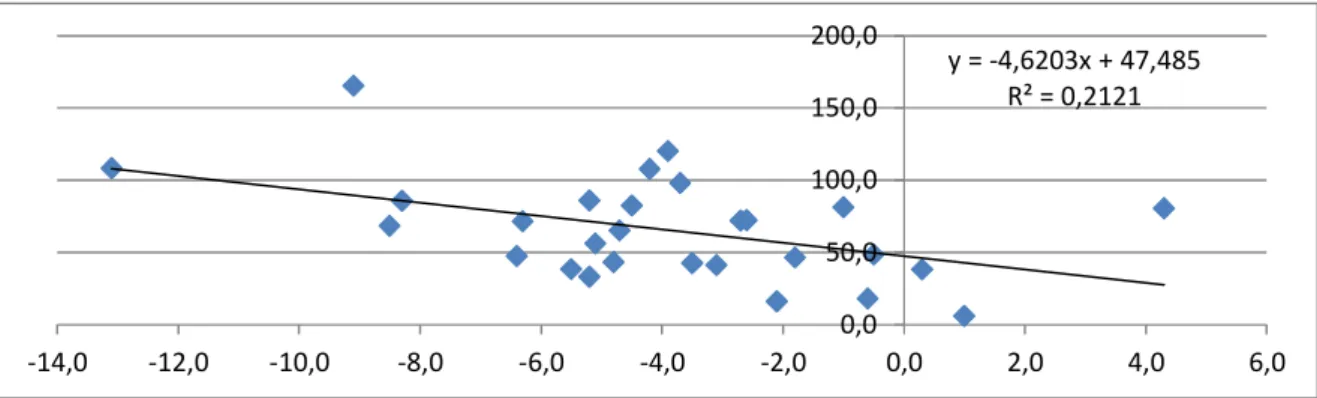
regression equation it can be seen the direct correlation between budget deficit and public debt, with countries with higher budget deficits having, as it is natural, higher levels of public debt.

Indeed, the highest levels of public debt are accompanied by the highest deficits. For instance, the budget deficit of Greece is almost 10% of GDP and the consequence - highest level of public debt. Similar case we can find in Ireland, Italy and UK. If Hungary is not considered (with a budgetary surplus), the correlation is more powerful, with almost 33% of countries with higher deficit having higher levels of public debt. This stylised evidence is in favour of reducing the budget deficit volatility for accomplishing a lower level of public debt.

Figure 1 Correlation between public debt and budget deficit in EU countries in 2011

y = -4,6203x + 47,485 R² = 0,2121

0,0 50,0 100,0 150,0 200,0

-14,0 -12,0 -10,0 -8,0 -6,0 -4,0 -2,0 0,0 2,0 4,0 6,0

Source: own computation based on Eurostat data.

(9)

8

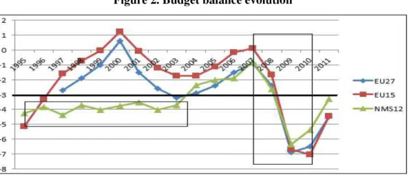
Figure 2. Budget balance evolution

Source: based on Eurostat data.

In the empirical analysis we are using a few categories of determinants of budget deficit volatility: macroeconomic determinants, fiscal variables, political variable and as a control variable population.

As a dependent variable we choose the budget deficit volatility computed as standard deviation (rolling window) for 4 years and 3 years, to take into account some features of the business cycle. Considering the fiscal variables included in the model also we compute the volatility of public revenue and expenditures for 4 years and 3 years.

Unlike, the previously studies, which were focused more on the political and institutional variables, this study is oriented more towards the relevance of economic and fiscal variables for explaining the budget deficit volatility. We consider these aspects because we want to reveal how it is feasible to reduce the budget deficit volatility if the economic conditions are changing and the government promotes a fiscal policy more oriented to reducing public debt – and issue faced by almost all EU member states in the present context.

(10)

9

BVit= 0+ 1*Xit+ 2*Yit+ 3Zit+ 4Wit+ it . (1)

In this baseline equation we introduce as the dependent variable the standard deviation of the budget deficit. As regressors we use a few categories of variables: Xit represents macroeconomic

variables such as the change of economic growth rate, GDP per capita, investment, inflation and unemployment rate; Yit are fiscal variables: expenditures, revenues, budget deficit, public debt,

expenditure volatility, revenue volatility; political variable (Polity 2), is noted with Zit and as a

control variable we choose the population Wit (see Appendix 1 for data description).

For the beginning we estimate a model with neither fixed nor random effects. Than we use fixed and random effects according with the result of Hausman test. Our estimates are for all EU 27 countries, but also we choose to divide the EU countries in two groups: the EU 15 – old member states and the NMS12 - new member states. To test the robustness of the results we also use for the EU 15 a dummy variable. Therefore,the purpose of the paper is to test the budget volatility determinants taking into account the conditions imposed by the Maastricht Treaty concerning the level of budget deficit of 3%, and 60% for public debt. In this regard we introduce this limit as a dummy variable to reflect how difficult is for the country which not accomplish this limits to reduce the budget volatility.

(11)

10

4. Empirical findings

Starting from the baseline equation we make the estimations considering the three categories of fiscal variables: revenues variable (results are in Table 1, 2 and 3), expenditures variables (results in Table 4 and 5), deficit and debt variable (results in 6 and 7). We choose to separate the fiscal regressors in distinctive equations to avoidmulticollinearity issues due to the fact that spending and revenues tend to evolve together.

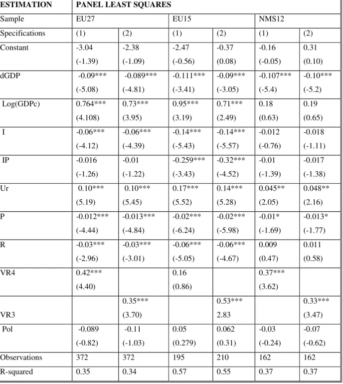
For the 4-year budget deficit volatility for all EU27 member states the most significant determinant is GDP change (see Table 1), because can reduce the budget deficit volatility. In particular, a percentage point increase of GDP would decrease the budget balance volatility by 0.11 percentage points for the EU 15 and 0.10 percentage points for the NMS12.

Table 1 – Insert here

GDP per capita is not significant for NMS12, only for EU27 and EU15 and if GDP per capita increases this also brings along higher budget deficit volatility. Increasing investment can be a solution for reducing the deficit volatility, but without a significant impact in NMS12. The unemployment rate increase can lead to higher deficit volatility, and this fact is quite relevant because of the powerful impact on both sides of the budget. If the unemployment rate increases the tax receipts decrease because less income taxes and social contributions are paid and, at the same time, public expenditures increase because the Government has to pay more unemployment benefits.

In the case of inflation, the results are significant for EU 15 and increasing the inflation seems to reduce the budget volatility. The control variable - population has a negative and significant impact on budget volatility. The political variables are not significant for the EU countries. For the NMS12 revenues are not significant for budget balance volatility, only the revenue volatility, a fact due to the lower level of tax receipts, instead, for the EU15 the revenue and their volatility is quite significant. If fiscal revenues are increasing than the volatility is reduced, but revenue volatility induces a higher volatility for the budget balance.

(12)

11

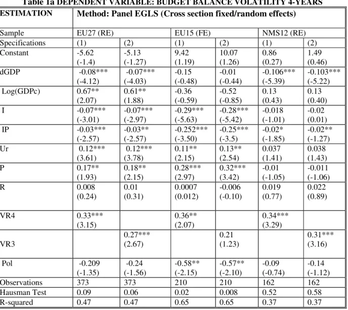
Table 1a reveals the same estimation like Table 1 based on fixed and random effects. We use Hausmann test for deciding between fixed or random effects. When the value of Hausman test is very high (p >0.05) we choose to use for estimation random effects, even if according to Clark and Linzer (2012) however, it does not necessarily follow that the random effects estimator is “safely" free from bias, and therefore to be preferred over the fixed effects estimator. In most applications, the true correlation between the covariates and unit effects is not exactly zero. The results concerning the significance are not very different from the previously, only small difference of estimators.

For testing the robustness of these results we choose to introduce a dummy variable that takes the value of one for the EU15 countries and zero for new member states NMS12.

Table 2 shows the results with the dummy variable for the EU 15 confirming the previous results. The 4-year revenue volatility is not significant for EU 15, instead the expenditure volatility is significant and with a direct impact on budget volatility. If we introduce in the model from Table 2 as regressor the expenditures variables (see equation 2) the R-squared is increasing at 73% and this fact reveals the powerful impact of expenditures side on the budget volatility. This means that the old members’ states have to maintain a stable level of their public expenditures to accomplish public finance stability. But the level of public expenditures is expected to increase especially for social protection expenditure and health as long as the ageing population impact can’t be diminished. If the expenditures volatility increases by one percentage point, then one expects an increase of 0.31 percentage points for the EU15 for the overall budget balance volatility.

(13)

12

revenues volatility. The impact of expenditure volatility is higher than revenue volatility and also more significant for all EU countries and this result is in accordance with Afonso & Jalles (2012).

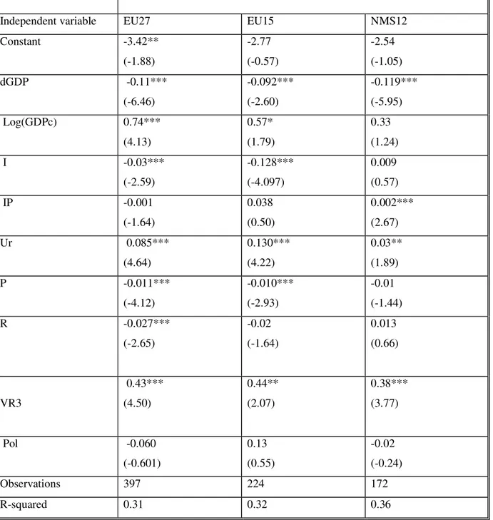
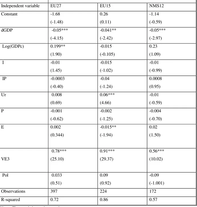
In Table 3 we present the results for the budget balance volatility computed for a rolling window of 3-years, for robustness. The results are quite similar with the previously computed 4-years volatility measure, and the impact of revenue volatility is higher in the EU15.

Table 3 –Insert here

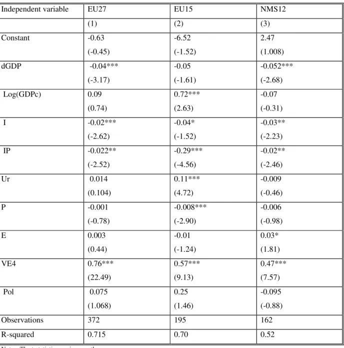
If we consider the expenditures variables, in Table 4, it can be observed the direct impact of expenditure volatility on the budget volatility, more powerful in the EU15 comparatively with the NMS12, a result confirmed also by the use of the dummy variable. In this case for the NMS12 countries investment increases can conduct to a lower volatility for the budget. In this case the change of GDP remains significant only for the EU27 and NMS12; and for the EU15 it becomes more significant the level of GDP per capita. This result is justified because the new member states have a higher economic growth rate and a reduced level of GDP per capita when compared with the old member states.

Table 4 –Insert here

If we test the determinants for the 3-years volatility (see Table 5) for the new member states, only the change in GDP and expenditure volatility remains significant. Based on this result we can identify as solutions for reducing the budget balance volatility on the short run, for new member states, the increase of economic growth rate and the reduction of expenditure volatility. The same solution can be relevant for the EU15, and in addition also reducing the unemployment rate, which is very significant for this group of countries.

Table 5 - Insert here

(14)

13

context also we choose to test the conditions imposed by Maastricht Treaty for the budget deficit level of 3% of GDP and for public debt 60% of GDP. For testing the impact of budget deficit and public debt under these conditions we choose to use a dummy variable with the value 1 for the countries which do not accomplish the requirements of the Maastricht Treaty. The results in Table 6 show the significant impact of the budget deficit level for EU27 and EU15 and also for those countries which have a deficit higher than 3% of GDP. For the new member states the level of budget deficit is not significant for the budget volatility.

Concerning the public debt for all EU countries the impact is significant; for the NMS12 an increase of public debt leads to higher budget volatility, but in the old new member states an increase of public debt can conduct to a decrease in volatility.

For the budget balance volatility for 3 years the budget deficit and public debt remains significant for EU27. For new member states increasing the level of public debt would lead to an increase of budget volatility.

5. Conclusions

This paper tries to provide new empirical evidence on the budget volatility determinants in a comparative view between old and new member states.

(15)

14

budget balance can be accomplished in the long run. For some countries, increasing budget revenues is a target quite difficult to accomplish because of the level of the underground economy with a significant share in the GDP, for instance in countries like Greece, Italy, Romania.

The unemployment rate impact on the budget volatility is significant and reducing the unemployment rate can be a solution for the budget balance stability. The results underline the necessity for the old members’ states to maintain a stable level of their public expenditures to reach public finances stability. But the level of public expenditures is expected to increase especially for social protection expenditure and health, as long as the ageing population impact can’t be diminished. Based on these results we can identify as solutions for reducing the budget balance volatility on the short run for new member states, mostly the increase in economic growth rate and the reduction of government spending volatility.

For the EU countries the aim is not to have lower budget volatility, and the target has to be reducing the level of public debt using as a mean a more stable budget balance, which means stable revenues and efficient public spending. If these two conditions are accomplished, than the effect will be lower budget volatility and derived from here a decreasing of budget deficit and more possibilities for reducing the level of public debt.

6. References

Afonso, A. and Furceri, D., 2010. "Government size, composition, volatility and economic growth," European Journal of Political Economy, Elsevier, vol. 26(4), pages 517-532, December.

Afonso, A. and Jalles, J.T., 2012. "Fiscal volatility, financial crises and growth," Applied Economics Letters, Taylor and Francis Journals, vol. 19(18), pages 1821-1826, December

Agnello, L. and Sousa, R. M., 2009. "The determinants of public deficit volatility,"

(16)

15

Bayar, A. H, 2001. “Entry and exit dynamics of ‘excessive deficits’ in the European Union”. Public Finance and Management, 1(1), 92-112.

Bayar, A. H. and Smeets, B., 2009. “Economic, Political and Institutional Determinants of Budget Deficits in the European Union”. CESifo Working Paper Series No. 2611. Available at SSRN: http://ssrn.com/abstract=1379604

Breunig, C., Koski, C., 2011. “Capture, Rupture, and Deadlock: Interest Groups and Budget Volatility”, Paper prepared for presentation at Comparative Agendas Project - 4th Annual Conference – Catania, June 23-25, 2011, available on-line at

http://comparativeagendas.files.wordpress.com/2011/06/breunig_koski_cap2011.pdf

Castro, V., 2007. "The Causes of Excessive Deficits in The European Union," The Warwick Economics Research Paper Series (TWERPS) 805, University of Warwick, Department of Economics.

Clark, T.S. and Linzer, D.A., 2012, Should I Use Fixed or Random Effects?, Working paper, available at http://polmeth.wustl.edu/mediaDetail.php?docId=1315, The Society for Political Methodology,

Cornia, G. C. and Nelson, R. D., 2010. “State Tax Revenue Growth and Volatility.”

Federal Reserve Bank of St. Louis Regional Economic Development, 6(1), pp. 23-58.

Roubini, N., and Sachs, J., 1989, “Political and Economic Determinants of Budget Deficits in the Industrial Democracies”, European Economic Review, 33, pp. 903-938.

Tujula, M. and Wolswijk, G., 2004. "What determines fiscal balances? An empirical investigation in determinants of changes in OECD budget balances, "Working Paper Series 422, European Central Bank.

(17)

16

Appendix 1 - Data description

Variable Description Unit Acronym Source

Gross domestic product, constant prices

Annual percentages of constant price GDP are year-on-year changes

Percent change

dGDP

IMF - WEO

GDP per capita Gross domestic product based on purchasing-power- parity (PPP) per capita GDP

Current international

dollar GDPc

IMF - WEO

Total investment Expressed as a ratio of total investment in current local currency and GDP in current local currency. Investment or gross capital formation is measured by the total value of the gross fixed capital formation and changes in inventories and acquisitions less disposals of valuables for a unit or sector.

Percent of GDP

I

IMF - WEO

Inflation, average consumer prices

Expressed in averages for the year, not end-of-period data. A consumer price index (CPI) measures changes in the prices of goods and services that households consume

Index

IP

IMF - WEO

Unemployment rate

The OECD harmonized unemployment rate gives the number of unemployed persons as a percentage of the labour force (the total number of people employed plus unemployed).

Percent of total labour force

Ur

IMF - WEO

Population For census purposes, the total population of the country consists of all persons falling within the scope of the census.

Millions Persons

P

IMF - WEO

General government revenue

Revenue consists of taxes, social contributions, grants receivable, and other revenue. Percent of GDP R Eurostat General

government total expenditure

Total expenditure consists of total expense and the net acquisition of nonfinancial assets. Percent of GDP E Eurostat The government deficit/surplus

Is the net borrowing/net lending of general government as defined in the ESA95. It is the difference between the revenue and the expenditure of the general government sector. The working balance is the most often used concept and measure of the country's

Percent of GDP

BD

(18)

17

budget deficit/surplus as it generally appears in public accounts and budgetary presentations. In other words, for example, for central government it should normally correspond to the budgetary outcome voted by the parliament.

Government consolidated gross debt

The Maastricht definition of debt is total gross debt at nominal value outstanding at the end of the year and consolidated between and within the sectors of general government.

Percent of GDP

Db

Eurostat

POLITY2 This variable is a modified version of the POLITY variable added

in order to facilitate the use of the POLITY regime measure in time-series analyses. It modifies the

combined annual POLITY score by applying a simple treatment, or “fix,” to convert instances of

“standardized authority scores” to conventional polity scores.

The POLITY score is computed by subtracting the AUTOC score from the DEMOC score; the resulting unified polity scale ranges from +10 (strongly democratic) to -10

(strongly autocratic).

Index

Pol

Polity IV database

Budget volatility 4-years

Computed as standard deviation for 4-years (rolling windows)

BV4 Budget volatility

3-years

BV3 Revenue

volatility 4-years

VR4 Revenue

volatility 3-years

VR3 Expenditure

volatility 4-years

VE4 Expenditure

volatility 3-years

(19)

18

Appendix 2

Table A2.1– Matrix correlation

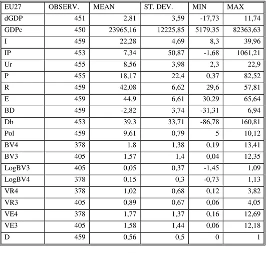
Table A2.2. Descriptive statistics for EU27

EU27 OBSERV. MEAN ST. DEV. MIN MAX

dGDP 451 2,81 3,59 -17,73 11,74

GDPc 450 23965,16 12225,85 5179,35 82363,63

I 459 22,28 4,69 8,3 39,96

IP 453 7,34 50,87 -1,68 1061,21

Ur 455 8,56 3,98 2,3 22,9

P 455 18,17 22,4 0,37 82,52

R 459 42,08 6,62 29,6 57,81

E 459 44,9 6,61 30,29 65,64

BD 459 -2,82 3,74 -31,31 6,94

Db 453 39,3 33,71 -86,78 160,81

Pol 459 9,61 0,79 5 10,12

BV4 378 1,8 1,38 0,19 13,41

BV3 405 1,57 1,4 0,04 12,35

LogBV3 405 0,05 0,37 -1,45 1,09

LogBV4 378 0,15 0,3 -0,73 1,13

VR4 378 1,02 0,68 0,12 3,82

VR3 405 0,89 0,67 0,06 4,05

VE4 378 1,77 1,37 0,16 12,69

VE3 405 1,58 1,44 0,06 12,18

(20)

19

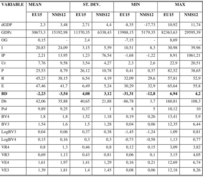
Table A2.3. Descriptive statistics in UE 15 and NMS12

VARIABLE MEAN ST. DEV. MIN MAX

EU15 NMS12 EU15 NMS12 EU15 NMS12 EU15 NMS12

dGDP 2,3 3,48 2,71 4,4 -8,35 -17,73 10,92 11,74

GDPc 30673,3 15192,98 11370,35 6338,43 13988,15 5179,35 82363,63 29595,39

OG 0,15 - 2,4 -7,15 - 8,69 -

I 20,83 24,09 3,15 5,59 10,51 8,3 30,98 39,96

IP 2,21 13,95 1,23 76,54 -1,68 -1,22 8,91 1061,21

Ur 7,76 9,58 3,54 4,27 2,3 2,6 22,9 20,51

P 25,53 8,79 26,12 10,78 0,41 0,37 82,52 38,65

R 45,23 38,15 6,54 4,19 32,09 29,6 57,81 52,9

E 47,46 41,7 6,49 5,24 30,29 32,9 65,64 55,8

BD -2,23 -3,54 4,08 3,12 -31,31 -12,8 6,94 4,2

Db 42,06 35,88 40,65 21,88 -86,78 3,7 160,81 108,3

Pol 9,89 9,25 0,37 1 8 5 10,12 10

BV4 1,8 1,8 1,52 1,18 0,19 0,26 13,41 5,9

BV3 1,54 1,6 1,5 1,28 0,04 0,06 12,35 6,44

LogBV3 0,04 0,06 0,37 0,38 -1,45 -1,24 1,09 0,81

LogBV4 0,15 0,16 0,3 0,3 -0,73 -0,58 1,13 0,77

VR4 0,8 1,3 0,46 0,8 0,12 0,15 3,09 3,82

VR3 0,69 1,13 0,43 0,81 0,06 0,1 3,15 4,05

VE4 1,61 1,97 1,41 1,29 0,16 0,21 12,69 6,74

(21)

20

Table 1DEPENDENT VARIABLE: BUDGET BALANCE VOLATILITY 4-YEARS

ESTIMATION PANEL LEAST SQUARES

Sample EU27 EU15 NMS12

Specifications (1) (2) (1) (2) (1) (2)

Constant -3.04

(-1.39) -2.38 (-1.09) -2.47 (-0.56) -0.37 (0.08) -0.16 (-0.05) 0.31 (0.10)

dGDP -0.09***

(-5.08) -0.089*** (-4.81) -0.111*** (-3.41) -0.09*** (-3.05) -0.107*** (-5.4) -0.10*** (-5.2)

Log(GDPc) 0.764***

(4.108) 0.73*** (3.95) 0.95*** (3.19) 0.71*** (2.49) 0.18 (0.63) 0.19 (0.65)

I -0.06***

(-4.12) -0.06*** (-4.39) -0.14*** (-5.43) -0.14*** (-5.57) -0.012 (-0.76) -0.018 (-1.11)

IP -0.016

(-1.26) -0.01 (-1.22) -0.259*** (-3.43) -0.32*** (-4.52) -0.01 (-1.39) -0.017 (-1.38)

Ur 0.10***

(5.19) 0.10*** (5.45) 0.17*** (5.52) 0.14*** (5.28) 0.045** (2.05) 0.048** (2.16)

P -0.012***

(-4.44) -0.013*** (-4.84) -0.02*** (-6.24) -0.02*** (-5.98) -0.01* (-1.69) -0.013* (-1.77)

R -0.03***

(-2.96) -0.03*** (-3.01) -0.06*** (-5.05) -0.06*** (-4.67) 0.009 (0.47) 0.011 (0.58)

VR4 0.42***

(4.40) 0.16 (0.86) 0.37*** (3.62) VR3 0.35*** (3.70) 0.53*** 2.83 0.33*** (3.47)

Pol -0.089

(-0.82) -0.11 (-1.03) 0.05 (0.279) 0.062 (0.31) -0.03 (-0.24) -0.07 (-0.62)

Observations 372 372 195 210 162 162

R-squared 0.35 0.34 0.57 0.55 0.37 0.37

Notes: The t-statistics are in parentheses.

*, ** and *** - statistically significant at the 10, 5 and 1% level, respectively.

(22)

21

Table 1a DEPENDENT VARIABLE: BUDGET BALANCE VOLATILITY 4-YEARS

ESTIMATION Method: Panel EGLS (Cross section fixed/random effects)

Sample EU27 (RE) EU15 (FE) NMS12 (RE)

Specifications (1) (2) (1) (2) (1) (2)

Constant -5.62

(-1.4) -5.13 (-1.27) 9.42 (1.19) 10.07 (1.26) 0.86 (0.27) 1.49 (0.46)

dGDP -0.08***

(-4.12) -0.07*** (-4.03) -0.15 (-0.48) -0.01 (-0.44) -0.106*** (-5.39) -0.103*** (-5.22) Log(GDPc) 0.67**

(2.07) 0.61** (1.88) -0.36 (-0.59) -0.52 (-0.85) 0.13 (0.43) 0.13 (0.40)

I -0.07***

(-3.01) -0.07*** (-2.97) -0.29*** (-5.63) -0.28*** (-5.42) -0.018 (-1.01) -0.02 (0.01)

IP -0.03***

(-2.57) -0.03** (-2.57) -0.252*** (-3.50) -0.25*** (-3.5) -0.02* (-1.85) -0.02** (-1.27)

Ur 0.12***

(3.61) 0.12*** (3.78) 0.11** (2.15) 0.13** (2.54) 0.037 (1.41) 0.038 (1.43)

P 0.17**

(1.93) 0.18** (2.15) 0.28*** (2.97) 0.32*** (3.42) -0.01 (-1.05) -0.011 (-1.06)

R 0.008

(0.24) 0.01 (0.31) 0.0007 (0.012) -0.006 (-0.10) 0.019 (0.77) 0.022 (0.89)

VR4 0.33***

(3.15) 0.36** (2.07) 0.34*** (3.29) VR3 0.27*** (2.67) 0.21 (1.23) 0.31*** (3.16)

Pol -0.209

(-1.35) -0.24 (-1.56) -0.58** (-2.15) -0.57** (-2.10) -0.09 (-0.74) -0.14 (-1.12)

Observations 373 373 210 210 162 162

Hausman Test 0.09 0.06 0.02 0.008 0.52 0.58

R-squared 0.47 0.47 0.65 0.65 0.37 0.37

Notes: t-statistics are in parentheses

(23)

22

Table 2 DEPENDENT VARIABLE: BUDGET BALANCE VOLATILITY 4-YEARS

Independent variable Dummy variable - EU15

(1) (Revenues) (2) (Exp) (3) R and E

Constant -1.57

(-0.62)

3.30 (2.14)

1.57 (0.97)

dGDP -0.09***

(-5.13)

-0.06*** (-4.99)

-0.04*** (-3.69) Log(GDPc) 0.64***

(3.06)

-0.24* (-1.81)

-0.075 (-0.55)

I -0.06***

(-4.13)

-0.01** (-1.93)

-0.015*** (-1.52)

IP -0.018

(-1.38)

-0.02*** (-3.01)

-0.02*** (-3.05)

Ur 0.09***

(4.96)

0.016 (1.26)

0.007 (0.56)

P -0.01***

(-4.57)

-0.003*** (-2.08)

-0.003** (-2.11)

R -0.03***

(-3.11)

-0.052*** (-4.29)

VR4 0.38***

(3.65)

-0.29*** (-3.90)

DVR4 0.17

(1.17)

-0.018 (-0.16)

E -0.006

(-0.86)

0.04*** (3.32)

VE4 0.59***

(13.56)

0.48*** (9.10)

DVE4 0.27***

(5.57)

0.31*** (5.36)

Pol -0.108

(-1.007)

0.05 (0.811)

0.03 (0.5)

Observations 372 372 372

R-squared 0.35 0.73 0.75

Wald test VE4=VR4 t-statistic: -1.66 *

The data sample includes yearly observations for the EU27 countries over the period 1995 to 2011. Budget volatility was obtained using standard deviation for 4 and 3 years (rolling windows)

(24)

23

Independent variable EU27 EU15 NMS12

Constant -3.42**

(-1.88)

-2.77

(-0.57)

-2.54

(-1.05)

dGDP -0.11***

(-6.46)

-0.092***

(-2.60)

-0.119***

(-5.95)

Log(GDPc) 0.74***

(4.13)

0.57*

(1.79)

0.33

(1.24)

I -0.03***

(-2.59)

-0.128***

(-4.097)

0.009

(0.57)

IP -0.001

(-1.64)

0.038

(0.50)

0.002***

(2.67)

Ur 0.085***

(4.64)

0.130***

(4.22)

0.03**

(1.89)

P -0.011***

(-4.12)

-0.010***

(-2.93)

-0.01

(-1.44)

R -0.027***

(-2.65)

-0.02

(-1.64)

0.013

(0.66)

VR3

0.43***

(4.50)

0.44**

(2.07)

0.38***

(3.77)

Pol -0.060

(-0.601)

0.13

(0.55)

-0.02

(-0.24)

R-squared 0.31 0.32 0.36

(25)

24

Table 4DEPENDENT VARIABLE: BUDGET BALANCE VOLATILITY 4-YEARS

(1) (2) (3)

Constant -0.63

(-0.45)

-6.52

(-1.52)

2.47

(1.008)

dGDP -0.04***

(-3.17)

-0.05

(-1.61)

-0.052***

(-2.68)

Log(GDPc) 0.09

(0.74)

0.72***

(2.63)

-0.07

(-0.31)

I -0.02***

(-2.62)

-0.04*

(-1.52)

-0.03**

(-2.23)

IP -0.022**

(-2.52)

-0.29***

(-4.56)

-0.02**

(-2.46)

Ur 0.014

(0.104)

0.11***

(4.72)

-0.009

(-0.46)

P -0.001

(-0.78)

-0.008***

(-2.90)

-0.006

(-0.98)

E 0.003

(0.44)

-0.01

(-1.24)

0.03*

(1.81)

VE4 0.76***

(22.49)

0.57***

(9.13)

0.47***

(7.57)

Pol 0.075

(1.068)

0.25

(1.46)

-0.095

(-0.88)

R-squared 0.715 0.70 0.52

(26)

25

Constant -1.68

(-1.48)

0.26

(0.11)

-1.14

(-0.59)

dGDP -0.05***

(-4.15)

-0.041**

(-2.42)

-0.05***

(-2.97)

Log(GDPc) 0.199**

(1.90)

-0.015

(-0.105)

0.23

(1.09)

I -0.01

(1.45)

-0.015

(-1.02)

-0.01

(-0.99)

IP -0.0003

(-0.40)

-0.04

(-1.24)

0.0008

(0.95)

Ur 0.008

(0.69)

0.06***

(4.66)

-0.01

(-0.59)

P -0.001

(-0.62)

-0.002

(-1.25)

-0.004

(-0.70)

E 0.002

(0.344)

-0.015**

(-1.94)

0.02

(1.50)

VE3

0.78***

(25.10)

0.91***

(29.37)

0.56***

(10.02)

Pol 0.033

(0.51)

0.09

(0.92)

-0.09

(-1.001)

R-squared 0.72 0.86 0.57

(27)

26

Independent variable

EU27 EU15 NMS12 EU27, with dummy variables Budget deficit <-3% of GDP Public debt >60% of GDP

Constant -2.35 (-1.18) -9.62*** (-2.63) 3.05 (1.07) -0.818 (-0.41) dGDP -0.02

(-1.28) 0.02 (0.76) -0.10*** (-4.66) -0.02 (-1.11) Log(GDPc) 0.68***

(3.98) 0.94*** (3.59) -0.05 (-0.18) 0.56*** (3.33)

I -0.06***

(-4.75) -0.09*** (-3.71) 0.01 (0.58) -0.06*** (-4.61)

IP -0.01

(-1.009) -0.18*** (-2.72) -0.01 (-1.45) -0.018 (-1.49)

Ur 0.089***

(4.88) 0.14*** (5.50) 0.05** (2.40) 0.07*** (4.26)

P -0.013***

(-5.16) -0.01*** (-4.89) -0.01** (-2.35) -0.01*** (-4.25)

Bd -0.17***

(-9.11) -0.21*** (-8.69) -0.02 (-0.74) -0.049 (-1.35)

DBD -0.149***

(-3.99)

DB -0.008***

(-4.48) -0.01*** (4.76) 0.01*** (3.02) -0.008 (-3.09)

DDB 0.0008

(0.36) Pol -0.17

(-1.71) 0.33 (1.85) -0.17 (-1.39) -0.21 (-2.19)

Observations 372 210 162 372

R-squared 0.42 0.61 0.36 0.45

Notes: The t-statistics are in parentheses. *, ** and *** - statistically significant at the 10, 5 and 1% level, respectively. The data sample includes yearly observations for the EU27 countries over the period 1995 to 2011. Budget volatility was obtained using standard deviation for 4 and 3 years (rolling windows)

DBD is a dummy variable with value 1, if the Budget deficit <-3% of GDP

(28)

27

Constant -3.01*

(-1.77)

-7.15

(-1.55)

0.47

(0.19)

dGDP -0.056***

(-2.93)

-0.07**

(-1.94)

-0.12***

(-5.10)

Log(GDPc) 0.63***

(4.07)

0.68**

(2.05)

0.08

(0.30)

I -0.04***

(-2.75)

-0.108***

(-3.37)

0.036*

(1.70)

IP 0.003***

(3.53)

0.09

(1.24)

0.002**

(1.95)

Ur 0.069***

(3.88)

0.14***

(4.62)

0.046**

(2.13)

P -0.012***

(-4.64)

-0.01***

(-2.92)

-0.01**

(-1.92)

Bd -0.16***

(-8.09)

-0.04

(-1.50)

-0.02

(-0.71)

DB -0.0006***

(-3.34)

-0.0018

(-0.64)

0.013***

(2.63)

Pol -0.132

(-1.36)

0.30

(1.33)

-0.12

(-0.99)

R-squared 0.36 0.31 0.33