Ricardo Alexandre Sacoto Martins

(1)

Ricardo Alexandre Sacoto Martins

Licenciado em Ciências da Engenharia Electrotécnica e de Computadores

Predicting Traffic Flow

Size and Duration

Dissertação para obtenção do Grau de Mestre em

Engenharia Electrotécnica e de Computadores

Orientador: Pedro Miguel Figueiredo Amaral, Professor Auxiliar, Faculdade de Ciências e Tecnologia,

Universidade Nova de Lisboa

Júri

Presidente: Doutor João Francisco Alves Martins - FCT/UNL Arguente: Doutor Luís Filipe Lourenço Bernardo - FCT/UNL

Vogal: Doutor Pedro Miguel Figueiredo Amaral - FCT/UNL

(2)

(3)

Predicting Flow Size and Duration

The Faculty of Sciences and Technology and the NOVA University Lisbon have the right, per-petual and without geographical boundaries, to file and publish this dissertation through printed copies reproduced on paper or on digital form, or by any other means known or that may be invented, and to disseminate through scientific repositories and admit its copying and distribution for non-commercial, educational or research purposes, as long as credit is given to the author and editor.

Este documento foi gerado utilizando o processador (pdf)LA_{TEX, com base no template “novathesis” [1] desenvolvido no Dep. Informática da FCT-NOVA [2].}

(4)

(5)

(6)

(7)

A

C K N O W L E D G E M E N T S

This section is dedicated to all the ones that went on this journey with me to elaborate this dissertation. One big special Thank You, to all of them!

In first place I would like to thank to Prof. Pedro Amaral for the opportunity to work on this theme, it’s a very compelling theme and it’s from the area that I like the most, the network department. I would also like to thank him for all the support, availability and help that was provided over this the past few months.

In second I would like to thank Faculdade de Ciências e Tecnologia da Universidade Nova de Lisboa , and the department of Electrical and Computer Engineering for giving the means to work on this thesis and also the opportunity complete my course. I would also like to acknowledge the support provided by FCT/MEC Project IT PEst- UID/EEA/50008/2013.

I would like to say a special thanks to my Mom Eunice, Dad Raul and sister Beatriz and of course my grandparents for all the help and support.

And for last but not least I would like to say thanks to all my friends that helped me through out this five years.

(8)

(9)

A

B S T R A C T

Current networks suffer from poor traffic management that leads to traffic congestion, even when some parts of the network are still unused. In traditional networks each node decides how to forward traffic based only on local reachability knowledge in a setting where optimizing the cost and efficiency of the network is a complex task.

Modern networking technologies like Software-Defined Networking (SDN) provide automation and programmability to Networks. In such networks control functions can be applied in a different manner to each specific traffic flow and a variety of traffic information can be gathered from several different sources.

This dissertation studies the feasibility of an intelligent network that can predict traffic characteristics, when the first packets arrive. The goal is to know the duration and size of flow to improve scheduling, load balancing and routing capabilities.

An OpenFlow application is implemented in an SDN Data Collecting Controller (DCC), that shows how the first few packets of a traffic flow can be gathered with scalability concerns and in a non-intrusive way.

The use of different classifiers such as Random Forest, Naive Bayes, Support Vector Machines, Multi-layer Perceptron and K-Neighbour for effective flow duration and size classification is studied. The results of using each of these classifiers to predict flow size and duration using the DCC gathered data are presented and compared.

Keywords: Software Defined Networking, OpenFlow, Data Collecting Controller, flow.

(10)

(11)

R

E S U M O

As redes actuais sofrem pela fraco gerenciamento de tráfego o que leva ao seu conges-tionamento, mesmo com algumas partes da rede ainda livres. Nas redes tradicionais cada nó decide como encaminhar o tráfego com base apenas no conhecimento de acessibilidade local onde a optimização do custo e eficiência da rede é uma tarefa complexa.

Tecnologias de redes modernas como SDN providencia automação e programabilidade das redes. Neste tipo de redes as funções de controlo podem ser aplicadas de diferentes maneiras ao tráfego de certos fluxos específicos e uma variedade de informação sobre este mesmo tráfego pode ser recolhida através de diferentes fontes.

Esta dissertação estuda a viabilidade de uma rede inteligente que consiga prever as características do tráfego, a partir dos primeiros pacotes. O objectivo é descobrir a dura-ção e tamanho de um fluxo para melhorar o agendamento, balanceamento de carga e capacidades de encaminhamento.

Foi implementada uma aplicação OpenFlow é numa SDN DCC, que demostra como os primeiros pacotes de um fluxo de tráfego podem ser recolhidos com preocupações de escalabilidade e de uma maneira não intrusiva.

Também foi estudado o uso de diferentes classificadores como Random Forest, Naive Bayes, Support Vector Machines, Multi-layer Perceptron e K-Neighbour para a classificação eficaz da duração e tamanho do fluxo. São apresentados e comparados os resultados do uso de cada um destes classificadores para prever o tamanho de um fluxo e a sua duração usando os dados recolhidos pelo DCC .

Palavras-chave: Software Defined Networking, OpenFlow, Data Collecting Controller, fluxo

(12)

(13)

C

O N T E N T S

List of Figures xv

List of Tables xvii

Acronyms xix

1 Introduction 1

1.1 Motivation . . . 2

1.2 Contributions . . . 2

2 Related Work 3 2.1 Software-Defined Networking . . . 3

2.1.1 Introduction . . . 3

2.1.2 SDN Architecture . . . 3

2.2 SDN using a Hierarchical Control Plane . . . 5

2.3 Gather of Data in SDN Networks . . . 7

2.4 OpenFlow . . . 7

2.4.2 Flow Table . . . 8

2.4.3 Types of flow entries . . . 9

2.4.4 Controllers . . . 10

2.5 Flow Prediction . . . 11

2.5.2 Machine Learning . . . 11

2.5.3 Classifiers . . . 12

2.5.4 Approaches in the literature . . . 16

3 DCC implementation 19 3.1 Introduction . . . 19

3.2 Topology . . . 20

3.3 Switch configuration . . . 21

3.4 OpenFlow application . . . 22

3.4.1 SwitchListener . . . 24

(14)

C O N T E N T S

3.4.2 PacketListener . . . 25

3.4.3 IpPacketHandler . . . 27

3.4.4 FlowEventListener . . . 27

3.4.5 DataStructure . . . 27

3.5 Python Script . . . 28

4 Results 31 4.1 Introduction . . . 31

4.2 Classification metrics . . . 31

4.3 Results . . . 32

4.3.1 Data Set . . . 33

4.3.2 Random Forest . . . 34

4.3.3 Naive Bayes . . . 35

4.3.4 Support Vector Machines . . . 36

4.3.5 Multi-layer Perceptron . . . 37

4.3.6 K-Neighbors . . . 38

4.3.7 Summary . . . 39

5 Conclusion 41 5.1 Conclusions . . . 41

5.2 Future Work . . . 42

Bibliography 45

(15)

L

I S T O F

F

I G U R E S

2.1 SDN architecture . . . 4

2.2 Architecture [1] . . . 6

2.3 Flochart detailing packet flow through an Openflow (v1.3) switch . . . 9

2.4 Floodlight architecture . . . 10

2.5 HP VAN SDN architecture . . . 11

2.6 Hidden Layer in MPL. . . 15

3.1 Architecture [1] . . . 19

3.2 Network . . . 20

3.3 HP-1 configuration . . . 22

3.4 Flowchart of the actions made by the OpenFlow application when apacket_in is received in a switch . . . 23

3.5 Rules installed in table 100 . . . 24

3.6 Rules installed in table 200 . . . 25

3.7 Flowchart of the class PacketListener . . . 26

3.8 Example of a TCP and UDP rule in table 200 . . . 27

3.9 Example of two flows saved in the csv file . . . 28

3.10 Histogram of the size of the flows . . . 29

4.1 Distribution of classes by size . . . 33

4.2 Distribution of classes by duration . . . 33 4.3 K-Neighbour average accuracy of the classes with values of K between 1 and 26 38

(16)

(17)

L

I S T O F

T

A B L E S

3.1 Classes for Size Classification . . . 29

3.2 Classes for Duration Classification . . . 29

4.1 Score for Size using Random Forest . . . 34

4.2 Score for Duration using Random Forest . . . 34

4.3 Score for Size using Naive Bayes . . . 35

4.4 Score for Duration using Naive Bayes . . . 35

4.5 Score for Size using Support Vector Machines . . . 36

4.6 Score for Duration using Support Vector Machines . . . 36

4.7 Score for Size using Neural Network . . . 37

4.8 Score for Duration using Neural Network . . . 37

4.9 Score for Size using K-Neighbour . . . 38

4.10 Score for Duration using K-Neighbour . . . 38

4.11 Average score for Size . . . 39

4.12 Average score for Duration . . . 39

(18)

(19)

A

C R O N Y M S

ANC Access Network Controller.

API Application Programming Interface. ARP Address Resolution Protocol.

ASIC Application-Specific Integrated Circuit.

CLI Command-line Interface. CNC Core Network Controller.

DBSCAN Density-based spatial clustering of applications with noise. DCC Data Collecting Controller.

DNS Domain Name System.

ECMP Equal-cost Multi-path Routing.

GMM Gaussian Mixture Model. GPR Gaussian Process Regression.

HMM Hidden Markov Model. HP Hewlett Packard.

HPE Hewlett Packard Enterprise. HTTP Hypertext Transfer Protocol.

IP Internet Protocol.

IPFIX IP Flow Information Export.

KNN K-Nearest Neighbors.

LSTM Long Short Term Memory.

(20)

A C R O N Y M S

MAC Media Access Control. MLP Multi-layer Perceptron.

MPLS Multiprotocol Label Switching.

NOS Network Operation System.

oBMM Online Bayesian Moment Matching.

REST Representational State Transfer. RNN Recurrent Neural Network.

SDN Software-Defined Networking. SVM Support Vector Machine. SYN Synchronize.

TCP Transmission Control Protocol. TLS Transport Layer Security.

UDP User Datagram Protocol.

VAN Virtual Application Network. VLAN Virtual Local area network.

(21)

C

H A P T E R

1

I

N T R O D U C T I O N

Modern networking technologies like SDN (Software Defined Networking) provide au-tomation and programmability to Networks. In such networks control functions can be applied in a different manner to each specific traffic flow and a variety of traffic information can be gathered from several different sources.

These characteristics open the possibility to perform intelligent resource management and traffic engineering, making use of knowledge that can be obtained via the available network data.

Particularly interesting is the possibility to perform routing decisions about traffic flows according to learned knowledge. For this to be useful we must be able to infer the characteristics of a particular traffic flow after only a few of its initial packets are transmitted. In the context of SDN networks this can only be done if the data (regarding a flow) that we need to make the decision can be collected at the network controller. SDN networks and particularly one of its most used southbound protocols, OpenFlow, provide data gathering mechanisms. Flow meta-data like Internet Protocol (IP) addresses Transport ports and other header values are easily obtained and initial flow packets can be sent to the controller where information like the size and time of arrival can be collected.

There are however some issues to take into account in this approach. The first has to do with the communication cost of sending initial flow packets to the controller, such cost can bring scalability problems especially in the controllers of switches that deal with a big numbers of flows. Another issue is the individual control of flows that can also lead to a scalability problem due to the limitation of the number of rules that one SDN switch can support. An important issue to deal with these scalability problems is the proper definition of what a flow is at each point of the network. This can range from packets that have the same 5-tuple (i.e. source IP address/port number, destination IP address/port number and protocol) to packets that have the same destination IP. The use of fine-grain flows

(22)

C H A P T E R 1 . I N T R O D U C T I O N

(5-tuple) should be limited to switches that deal with a small amount of traffic. For core switches with heavy traffic flows should be defined more broadly.

Regarding the communication cost the use of learning based on packet data can be restricted to access switches (where flows enter the network).

One way to achieve both these things is to use a hierarchical control plane where different controllers control different parts of the network.

1.1 Motivation

Two of the most interesting metrics for network control are flow duration and flow size. They can be used to improve load balancing, scheduling and routing capabilities. This is a challenging task, since each flow has is own pattern and is continuously changing.

In this thesis we study the possibility to predict flow information from its first few packets. We aim to use this information for efficient traffic distribution in an SDN network with a scalable distributed control plane. In order to achieve this the information that is used to train the predictors must be available in the SDN controllers, this means that the training data to be gathered must contain the same flow data features that are observable at the SDN controller of the Access node where a Flow originates. We therefore explore the possibility to obtain training data in a scalable and non-intrusive way in the SDN network. And then study the feasibility of using this data to train classifiers to be used for flow online classification in the access nodes SDN controller.

1.2 Contributions

In a previous work [1] a distributed control plane SDN architecture has proposed. In this thesis it is expanded by proposing mechanisms for traffic data collection without impact in the network performance. The previous architecture uses a distributed control plane with two different control points: the Core Network Controller (CNC), that controls core switches and the Access Network Controllers (ANCs) that control access switches. In this work we add a third control point, the DCC, that controls some of the ports of a set of core switches in the network and collects traffic data outside of the communication path.

An implementation of this new third controller was made in a lab network and was used to retrieve a dataset from live traffic flows produced by students using the network.

The obtained dataset is described and a study and evaluation of several types of classi-fiers is also conducted. Finally we present the results of using those classiclassi-fiers to classify flows according to their size and duration and discuss its applicability for online network management.

(23)

C

H

A

P

T

E

R

2

R

E L AT E D

W

O R K

This Chapter starts by briefly describing SDN and the Openflow protocol. It then presents the distributed control plane SDN architecture that was extended in this work. Finally we review related work regarding the problems of data gathering and online flow classification in SDN networks.

2.1 Software-Defined Networking

2.1.1 Introduction

The term SDN was originally created to represent the ideas and work around OpenFlow at Stanford University [2]. As originally defined, SDN refers to a network architecture where the forwarding state in the data plane is separated from the control.

The Data plane refers to the hardware part where forwarding of packets takes place, and the control plane refers to the software part where all network intelligence lies.

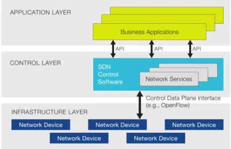
2.1.2 SDN Architecture

There are four pillars that define the SDN network architecture [3]:

1. The control and data planes are decoupled. With this network devices will become forwarding elements.

2. Forwarding decisions are made according to rules defined by the control plane and installed in the forwarding plane.

3. The control logic resides in one or more SDN controllers, also known as Network Operation System (NOS).

(24)

C H A P T E R 2 . R E L AT E D W O R K

4. The network is programmable through software applications on top of the NOS, which interacts with the underlying data plane devices.

Figure 2.1: SDN architecture

2.1.2.1 Control Plane

The control plane/controller presents an abstract view of the complete network infrastruc-ture, enabling the administrator to apply custom policies/protocols across the network hardware. However there are problems with scalability related to the number of hardware devices controlled by a single controller instance. The two main issues are the cost of high churn in communication between controller and forwarding elements and the limits in the number of forwarding rules supported in the hardware. This can be alleviated either with horizontally distributed controllers, which are independent controllers with state replica-tion, or vertically using distributed controllers, that are distributed hierarchically which means they cooperate between them and each one has its functions.

2.1.2.2 Northbound application interfaces

The northbound Application Programming Interfaces (APIs) represent the software inter-faces between the software modules of the controller platform and the SDN applications running on top of the network. These APIs expose universal network abstraction data models and functionality for use by network applications. The northbound APIs are open source-based.

(25)

2 . 2 . S D N U S I N G A H I E R A R C H I C A L C O N T R O L P L A N E

2.1.2.3 East–West protocols

In the case of a multi-controller-based architecture, the East–West interface protocol is responsible to manage interactions between the several controllers [4].

2.1.2.4 Data plane and southbound protocols

The data plane represents the forwarding hardware in the SDN network architecture. Because the controller needs to communicate with the network infrastructure, it requires a Southbound API to provide communication between the controller and the forwarding elements. The most popular protocol for this Southbound API is the OpenFlow protocol. The following section explains OpenFlow and its architecture.

The decoupling between control and forwarding brings two main advantages. The first is that network evolution is simpler with simple changes in software at the controller com-pared to the traditional configuration and/or firmware changes in a multitude of devices of possibly different vendors. The second is that controllers can have a broader view of the network state compared with the local knowledge of a single network element which can be used for smarter decisions. However, there are some problems with scalability in SDN, such the limited amount of rule space in the switches and the delay cost and consistency problems of excessive controller-switch communication. These problems are mainly con-cerned with the communication costs between controllers and network elements and with the limited amount of space to install rules in the hardware of the forwarding elements. In a previous work performed at the telecommunications group an SDN architecture with a distributed Hierarchical control plane was proposed as way to overcome this scale issues. It is presented in the next section.

2.2 SDN using a Hierarchical Control Plane

In [1] an SDN network architecture is proposed that uses a logically hierarchical control plane that separates the control plane of the core switches, where switches deal with more traffic, from the control plane of the access switches, that are in the edge of the network, and only deal with the traffic entering the network in that point. This approach helps in overcoming several scalability issues in SDN networks, like the limited amount of rule space in the switches and the delay cost and consistency problems of excessive controller-switch communication. In figure 2.2 there is a representation of the architecture proposed in that work.

(26)

Figure 2.2: Architecture [1]

The control plane is separated between the CNC and the ANCs. The CNC controls the core switches, where a high level of controller-switch communication should be avoided. Applying fine-course control logic (e.g. using 5-tuple flow based forwarding) should also be avoided because it would lead to a high number of forwarding rules. ANCs control the switches at the edge of the network (access switches), which connect the network to other networks or to hosts, and only deal with traffic that enters/exits the network in that point. This means that their rule space does not need to scale so much as in the previous case and flow based forwarding rules can be used. A higher degree of communication between these access switches and their controller can also exist since we are only dealing with the traffic that originates in those edges. Both control plane levels can be physically distributed by several controllers each one controlling a group of switches. The CNC calculates a set of paths between the access switches with any given algorithm (e.g shortest paths) and proactively installs one forwarding rule for each available path for any given destination. Forwarding rules are therefore per-path, per-destination consisting of OpenFlow Flow Entries with a match clause that matches destination IP address and Multiprotocol Label Switching (MPLS) tag (to distinguish between paths for the same destination). The ANC performs reactive flow distribution (i.e. deciding after the first packet of the flow) among those paths by tagging the flow traffic with the MPLS tag of the chosen path.

This work is motivated by this architecture and the Data gathering capabilities of SDN. We study ways to apply flow knowledge to the architecture,specifically the use of flow size and duration prediction to be used for reactive flow distribution decisions performed in the ANC. The first step to achieve this is to obtain traffic and flow data. In the next section we review the data gathering capabilities of SDN networks. We clarify how Openflow works and which controllers were used. We then explain three types of machine learning and five classifiers that were tested. Finally we discuss ideas from other literatures.

(27)

2 . 3 . G AT H E R O F D ATA I N S D N N E T W O R K S

2.3 Gather of Data in SDN Networks

SDN networks can provide fine-grained forwarding rules (e.g. OpenFlow flow entries) that determine how a packet is handled according to the information in the packet headers. It also provides built-in forwarding rule statistics like packet and byte counts. Besides, OpenFlow (a standard controller switch communications protocol) can be used in other ways to obtain relevant data. Forwarding rules have timers to control their duration. It is possible to configure a flow to expire when packets with a specific set of characteristics (Match fields) stopped arriving at the network. This can be used to provide information regarding the duration of a traffic flow. Rules can also be used to instruct devices to send packets with some predefined characteristics to the controller, where payload related information can be extracted.

For example when the first packet comes we can gather the information from its header and with that we create a rule for the controller to gather the firstN data packages that come with a matching header.

Dedicated data gathering protocols based on the IP Flow Information Export (IPFIX) standard could also be used (if supported by the switches) as an alternative [5]; or parallel data source in SDN networks. To be able to predict flow characteristics online, one must be able to do so very quickly so that policy or routing decisions based in that information still affects the majority of the flow traffic. This means that the Machine Learning algorithms used for that purpose must be integrated into the network control logic in a scalable and seamless way. If we use SDN mechanisms only, data are received directly in the controller where we can use them to classify a flow after its first initial packets and act immediately in the network. This means that SDN mechanisms must be used at least at this stage even if training data-sets for the Machine Learning algorithms are obtained by other means. IPFIX could, for example, be used to collect data for offline training. However, it cannot provide payload information related features like the ones we can obtain in an SDN controller.

2.4 OpenFlow

There are several protocols to use inside a Southbound API, but OpenFlow was one of the firsts standards used in SDN, and one of the most used today. OpenFlow enables the SDN controller to directly interact with the forwarding plane of the network devices such as routers and switches. The most important aspect of OpenFlow for this thesis is the fact that it can gather several statistics from such as number of packets, byte count and others. In this thesis OpenFlow protocol version 1.3 was used, this was the most recent version supported by our hardware.

(28)

2.4.2 Flow Table

A Flow Table consists of a list of Flow entries also known as rules, that indicate the switches how to behave when they receive a packet that matches a certain rule. The OpenFlow entries are stored in a flow table, each flow entry is composed by:

• Match Fields: Used to define the packets that match the rule. Matches can be made on things like the packet headers and ingress port.

• Priority: Used to distinguish priority between rules.

• Counters: Maintain statistics about the byte count and the number of packets and that match a rule.

• Instructions: Used to define the actions to apply to the matched packet and/or pipeline processing instructions.

• Timeouts: Maximum amount of time or idle time before flow is removed by the switch.

• Cookie: Used to identify flow entries.

• Flags: Used to define how flow entries are managed.

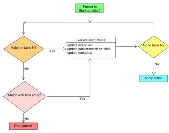
Every captured packet by the switch is send to the controller by in a form of a packet_in message. The processing of these packets via flows in OpenFlow 1.3 protocol through a switch can be seen in a flowchart in Figure 2.3.

(29)

2 . 4 . O P E N F L O W

Apply action

Drop packet Match in table N?

Match with flow entry?

Go to table N? Execute instructions:

update action set

update packet/match set field update metadata

Packet In Start at table 0

No

Yes

No No

Yes

Figure 2.3: Flochart detailing packet flow through an Openflow (v1.3) switch

If one of the rules inside the entry table matches the packet_in there is an associated instruction, that performs a certain action. This instruction can be a simple action like sending the packet_in to another table, or it can be a set of actions. For instance, if a packet matches the rule that packet will forward to a certain port instead of just being forwarded like a normal packet, and it will be foward to the controller. If no match is found in the table the packet is dropped [6]. It is possible to modify this default action regarding the unmatched packets using the flow miss table. This can be changed to send the packet_in to the controller or to a specific table.

2.4.3 Types of flow entries

Flow entries are used to install Openflow rules in the switches. These entries can be classified in two different types: proactive and reactive. The proactive ones are installed as soon as the switch connects to the network - these rules are more generic since it will treat all the packets in the same way. One example could be a rule that sends to the controller all traffic that is Transmission Control Protocol (TCP). The reactive flow entries will only create rule when the switch receives a packet. This rule will use the header of the packet to create the matchfields necessary for the rule. Both of theses types of flow entries were used in this thesis.

When considering which type of flow entries to use, we also have to consider their granularity since with a more specific rule we can gather specialized data. However it

(30)

will also create a flow overhead in the switch due to the number of rules that would be created for every packet that has different headers. In this thesis some rules have a large granularity since they embrace all TCP or User Datagram Protocol (UDP) traffic, but others are more specific such as the ones to gather the duration and the total size of specific flow.

2.4.4 Controllers

The number of software-defined controllers available in the market has increased greatly in the last few years. Nowadays, it is possible to find proprietary controllers as well as open source controllers. In this thesis two different controllers were tested, Floodlight and the Aruba VAN controller.

2.4.4.1 FloodLight

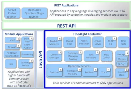
The Floodlight Open SDN Controller is an open source Java-based OpenFlow Controller. This controller is compatible with non-Openflow and Openflow networks. It’s based on a modular architecture. The version used was the most recent at athe time, version 1.3. The Floodlight Controller realizes a set of common functionalities to control and inquire an OpenFlow network, while applications on top of it implement different features to solve different user needs. Figure 2.4 shows the Floodlight architecture. Applications can be built as new modules that are compiled with the rest of the Floodlight modules, or they can be built externally and use the Floodlight Representational State Transfer (REST) API [7].

Figure 2.4: Floodlight architecture

After creating a program to write the rules on the switches and on the controller, Floodlight had some incompatibility issues with the Hewlett Packard (HP) switches that we had. Even thought the rules were written in simulations such as Mininet, the switches

(31)

2 . 5 . F L O W P R E D I C T I O N

didn’t had any rules. After some troubleshooting and trying some plugins in floodlight and in the switches, the problem stayed and for this reason we couldn’t use this type of controller.

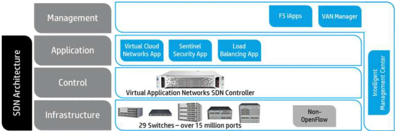
2.4.4.2 Aruba VAN SDN

Aruba Virtual Application Network (VAN) SDN Controller is another Java-based Openflow Controller made by Aruba Networks. It is an updated version of the previous controller of Hewlett Packard Enterprise (HPE) VAN SDN that was renamed after the acquisition of the Aruba Company by HPE. This controller is aimed for enterprise and campus networks.

The used version is at the time of this writing, the most recent, version 2.8.

Figure 2.5: HP VAN SDN architecture

This controller was the one chosen in the end due to the incompatibility with HP switches from the previous controller.

2.5 Flow Prediction

In this section we cover the related work on the problem of classifying flow size and duration. We start by explaining the machine learning algorithms and concepts that can be used to infer flow and traffic knowledge from the gathered data, and then proceed to describe several approaches on the application of these algorithms to Network traffic data.

2.5.2 Machine Learning

Machine Learning algorithms can be used to infer relationships and extract knowledge from gathered data. There are three main approaches for learning algorithms.Supervised Learning, Unsupervised Learning and Reinforcement Learning [8].

• Supervised Learning: Supervised learning consist in obtaining outcome variables (or dependent variables) which are predicted from a given set of predictor variables

(32)

(data features). Using these set of variables, a function that maps inputs to desired outputs is generated in what is called the training process. The process finishes when the model achieves a desired level of accuracy on the training data . Examples of Supervised learning algorithms are: K-Nearest Neighbors (KNN), Random Forest, Decision Tree and Logistic Regression.

• Unsupervised Learning: Unsupervised Learning is a data-driven knowledge discov-ery approach that can automatically infer a function that describes the structure of the analysed data or can highlight correlations in the data forming different clusters of related data. Examples of algorithms include: K-Means, Density-based spatial clustering of applications with noise (DBSCAN) and A priori.

• Reinforcement Learning: These algorithms are trained to make specific decisions. The goal is to discover which actions lead to an optimal configuration. This is done by learning from past experiences. As an example, a network administrator can set a target policy, for instance the delay of a set of flows in an SDN Network. Then an algorithm results in actions on the SDN controller that change the configuration and for each action a reward is received, which increases as the in-place policy gets closer to the target policy. Ultimately, the algorithm will learn the set of configuration updates (actions) that result in such target policy (e.g. Markov Decision Process).

2.5.3 Classifiers

In the following sections we pressed several supervised classifier algorithms. We start by describing how each algorithm works and then make a summary of the algorithm advantages and disadvantages.

2.5.3.1 Random Forest

Random forest is a supervised classifier that consists in creating a set of decisions trees from a randomly selected subset of samples from the training set. When a node is split during the construction of a tree, the split that is chosen is not the best as in decision trees, but instead the best among a random subset of features. For the N trees that are created, N random subsets of features are used, which increase the diversity of the forest. When it comes the time to make a prediction, it takes into consideration all individual decision tree predictions and chooses the most voted. Due to this random factor, bias in the forest tends to increases, but this factor is counter measured with averaging from all trees decreasing the variance, becoming a better model than decision trees[9].

A variant form of this classifier is called Extremely Randomized Trees and it has two main differences. First, when choosing variables at the split phase (when dividing a node in two other nodes), samples are drawn from the entire training set instead of a bootstrap sample( is a smaller sample randomly selected from a larger sample), and second, splits

(33)

are chosen completely at randomly from within the range of values in the sample at each split. It results in more "ramifications"in each tree.

The main advantages of using Random Forest are:

• Use of decorrelated trees.

• Good for parallel or distributed computing.

But there are some disadvantages such as:

• Poor performance on imbalanced data (rare outcomes).

• Lack of an interpretable model, compared to decision trees.

2.5.3.2 Naive Bayes

The Naive Bayes algorithm consists in applying the Bayes theorem with the assumption of independence between every pair of features. In simple terms, a Naive Bayes classifier assumes that the presence of a particular feature in a class is independent to the presence of any other feature.

Given a class variable y and a dependent feature vector X = x₁, x₂, ..., xn , Bayes

theorem, provides a manner of calculating posterior probabilityP(y|X)fromP(y),P(X)

andP(X|y)with the following rule [10]:

p(y|X) =p(y)×p(X|y)

p(X)

In the equation above,

P(y|X) represents the posterior probability of class y (target) given predictorX

(features).

P(y)constitute the prior probability of class.

P(X|y)states the probability of predictor given class.

P(X)indicates the prior probability of predictor.

After calculating the posterior probability for each class, for the given features, the class with highest posterior probability is the outcome of prediction.

The main advantages of using Naive Bayes are:

• Good performance with multi classes.

• Easy and fast to predict.

• Doesn’t need to be all numeric variables; features can come in variables.

(34)

• Zero Frequency issue, it happens when a variable as a condition that was not ob-served in the data set and the model will assign zero as the probability, thus is unable to predict the class. This can be solve with smoothing techniques, such as Laplace estimation.

• On the other side, Naive Bayes is also known as a bad estimator.

• It assumes independent predictors.

2.5.3.3 Support Vector Machines

Support Vector Machines (SVMs) are a set of supervised learning methods that can be used for classification, regression and outliers detection. As a classifier it is considered a discriminative classifier formally defined by a separating hyperplane. In other words, given labelled training data (supervised learning), the algorithm outputs an optimal hyperplane which classifies new sets [11].

The main advantages of using SVMs are:

• Effective in high dimensional spaces.

• Effective when the number of dimensions is greater than the number of samples.

• Memory efficient.

• Versatile: different Kernel functions can be specified for the decision function.

• Over-fitting when number of features is much greater than the number of samples.

• Memory requirements in large scale samples.

If the number of features is much greater than the number of samples, avoiding over-fitting is crucial by choosing the right Kernel functions and regularization term. SVMs do not directly provide probability estimates. These are calculated using Platt scaling with an expensive five-fold cross-validation. These methods transform the outputs of a classification made by SVM into a probability distribution over the classes.

2.5.3.4 Neural Network - Multi-layer Perceptron

A Multi-layer Perceptron (MLP) is a supervised learning algorithm that learns a function

f(·) :Rd_→_Rs_{by training on a designated dataset, where}_d_{is the number of dimensions}

for the inputs andsthe number of dimensions for outputs. Given a set of featuresX=

x1, x2, ..., xd and a target y, it can learn a non-linear function for either regression or

classification [12]. The main difference between logistic regression and MLP is that in the latter there can be one or more hidden layers (non-linear), between the input and the output. In figure 2.6 we can visualise an MLP with a hidden layer:

(35)

Figure 2.6: Hidden Layer in MPL.

At the left side of figure 2.6, we can observe several inputs entering in a neuron. A neuron consists in a computational function that receives an input signal, sums with its weights ( strength/amplitude of a connection between the two nodes) and produces an output signal using an activation function. The hidden layer receives those output signals and applies a non-linear function. Those values are then received by the output layer that transforms them into an output value.

The main advantages of using MLP are:

• Effectiveness in high dimensional spaces.

• Capability to learn non-linear models

• Online learning, learning models in real-time.

• Complicated to configure, due to hidden neurons, layers and their iterations.

• It’s sensitive to feature scaling.

• Hidden layers have a non-convex loss function where there exists more than one local minimum. Therefore different random weight initializations can lead to different validation accuracy.

2.5.3.5 Nearest Neighbors

Another supervised learning algorithm is Nearest Neighbors classifier. The principle behind it consists in finding data samples closest in distance to each data point, forming clusters of similar data points that can then be labelled. A new point is considered to have the label

(36)

of the closest cluster. The number of samples can be configured to be constant (K-Nearest Neighbor learning), or vary based on the local density of points (Radius-Based Neighbor learning). This constantKis a typically small positive integer. The distance can, in general, be any metric measure such as standard Euclidean distance which is the most common choice. In this case of classification, the object will be classified by a majority vote of its neighbours, with the object being assigned to the most common class among its k nearest neighbours. Neighbors-based methods are known as non-generalizing machine learning methods, since they simply "remember" all of its training data [13].

The main advantages of using K-Nearest Neighbors are:

• Very easy to use and implement.

• Handles multi-class cases.

• Can quickly respond to changes in input.

• Stores all of the training data.

• Computation time.

• Sensitive to irrelevant features and the scale of the data.

2.5.4 Approaches in the literature

A flow classifier that classifies flows in to two different classes is proposed in [14] . The two classes of flows, the elephants (heavy) and mouse (light) are separated by a pre-defined threshold. Above it flows are considered an elephant flow, and bellow a mouse flow.

The classifier uses several data of each flow, such as Source IP, Destination IP, Source Port, Destination Port, Transport Protocol, the size of the first three packets after synchro-nization and Server vs Client. This last parameter is only used when flow protocol is TCP and it represents who initiated the flow if is a request by the client or a response by the server. The data is gathered using software defined networks mechanisms. The first packet (after synchronization) contains the data mention above, the other two packets are only needed to gather their size.

The paper studies several types of regression algorithms, namely, Gaussian Process Regression (GPR), Online Bayesian Moment Matching (oBMM) and Gaussian Mixture Models (GMMs). The most promising results were obtained using data from the first three packets with GPR, with a 14.17% improvement in elephant flows and 0.59% in mice flows compared with Equal-cost Multi-path Routing (ECMP).

This approach is similar to one of the goals of this thesis (flow size classification), however instead of just two classes we pursue a classification with more classes.

In [15], flow size prediction is performed based on past observations with the use of a Hidden Markov Model (HMM).

(37)

A HMM is a statistical Markov model in which the system being modelled is assumed to be a Markov process with unobserved (i.e. hidden) states. In simpler Markov models (e.g. Markov Chain), the state is directly visible to the observer, and the state transition probabilities are the only parameters. In the hidden Markov Model, only the output is visible and the state must be inferred. Each state has a probability distribution over the possible outputs.

In [15] it is proposed to use HMM to describe the relation between of the flow count and the flow volume but also the temporal dynamic behaviour between both. To train this model, Long Short Term Memory (LSTM) is used with Recurrent Neural Network (RNN) and KNN.

In this HMM, the hidden variable that we want to know is the traffic volume and the known variable is the flow statistic which in this case is the flow count. Flow count represents the number of flows for a certain time interval.

A comparison of the prediction mean square error values is made between KNN and RNN [15] with both obtaining similar results but with KNN outperforming RNN by 0.05 in the larger set with 300 training samples and 100 test samples. Both of the algorithms had always prediction errors bellow 0.5, which indicates less than half of the variance of the time series. Between these two algorithms if processing power weren’t an issue we would go with KNN since is more precise, otherwise RNN since is a less complex algorithm.

However this method can only take into account the number of flows in a sequential interva. For the intervaltit determines the volume of the traffic for interval t+1(future traffic), which means that in order to predict future traffic we need information from the previous one. This can be very expensive to obtain in big networks. Another issue is network traffic is changing dynamically which means the behaviour of the transmission could also change. To adapt to this change the algorithm implemented ,KNN or RNN would need to be learning in real time.

In [16, 17], flows are classified into safe flows and malware generated flows. In that work, Netflow, is used to gather information from the packets in the flows that traverse the network,including data such as the 5-tuple (i.e. source IP address/port number, destination IP address/port number and protocol). Four main data features are also collected: the sequence of packet lengths and times and their byte distribution, the Transport Layer Security (TLS) handshake metadata and the initial data packet. These four features are collected by using Application-Specific Integrated Circuit (ASIC), architecture that provides the ability to collect this data without mitigating the network. With that data , malware inside encrypted traffic is detected [17]. TLS, Domain Name System (DNS), and Hypertext Transfer Protocol (HTTP) metadata is collected and correlated. This data is then used to accurately classify as malicious, TLS network flows features of the TLS protocol are aggregated with DNS and HTTP features from contextual (related) flows and this is shown to improve the discriminatory information contained in the data. Anl1-logisticts regression was used to pinpoint malicious patterns in encrypted traffic to help identify threats and improve incident response.

(38)

(39)

C

H

A

P

T

E

R

3

D C C

I M P L E M E N TAT I O N

3.1 Introduction

Taking into account the figure 3.1 previously proposed , we needed a method that would permit us to gather traffic information without interfering with the network. For this reason, we decided to implement a DCC with a mirror of the important traffic, in our case the traffic that would go to/come from the gateway. By implementing it in this manner we would prevent delays in the traffic forwarding while collecting the data and build the overhead on communications between the controller and the switches. The only traffic that would be affected was the mirrored traffic. This implementation would also make the network more scalable.

Figure 3.1: Architecture [1]

(40)

C H A P T E R 3 . D C C I M P L E M E N TAT I O N

In this section we start to explain the topology used to implement the DCC and the configurations needed in the switch.

We also explain in detail how the OpenFlow application installed in the DCC was implemented and how we can gather from the first few packets the Date, Ethernet Type, source Media Access Control (MAC) address, source IP, destination IP, Protocol, source Port, destination Port, Byte count, duration, number of packets, the size of the first packets and their arrival times.

Finally, we describe the Python script that was used to train and implement the classi-fiers.

3.2 Topology

An SDN aplication for the DCC controller was developed. The application collects training data about the data flows that traverse the controlled switches. In order to obtain data from an existent non SDN network, an SDN controlled switch was connected to the gateway of a small network that connects two rooms from the university campus.

Since both of these rooms (Labs 3.5 and 3.9) are support rooms for MSc. and PhD. students that are developing their projects or thesis inside the telecommunication section, the process had to be transparent to the production Network.

This was done by placing the DCC controlled switch in the uplink path from the network to the Gateway, like depicted in figure 3.1. The Switch then mirrors the traffic headed to the gateway to an Openflow controlled port. In this way traffic is copied to the Openflow port and follows its path to the gateway without further interference. This type of deployment allows the gathering of data in non SDN networks.

This can also be useful when deploying the architecture described in [1] in a previously existent network, since data for training can be gathered ahead of the full implementation of the SDN architecture.

Figure 3.2: Network

(41)

3 . 3 . S W I T C H C O N F I G U R AT I O N

3.3 Switch configuration

A HP 3800-24G-PoE+-2SFP+ Switch (HP-1) was used as the DCC controlled SDN switch. The switch was used in the Virtualization Mode [18]. This mode allows OpenFlow Virtual Local area networks (VLANs) to coexist in the same switch with non-OpenFlow VLANs. To make this possible, OpenFlow instance is configured to associate a VLAN to Openflow and to insert the IP address of the controller.

An alternative to Virtualization mode could be Aggregation mode. However in this mode all VLANs on the switch must be part of the OpenFlow instance, since we needed other VLANs active on that same switch to connect the uplink from the existing network to the gateway. To mirror the traffic, we needed to use the virtualization mode.

This HP switch had a mode called hybrid mode. This mode determines which packet-forwarding decision are made by controlled OpenFlow switches and which of these de-cisions are made by the controller itself. When enabled, the controller delegates normal packet-forwarding to the controlled switches, but overrides these switches for non-standard packet-forwarding decisions required by installed applications for specific packet types. Packets in flows that the controller does not examine or direct are forwarded through nor-mal switching operations without controller intervention. When disabled, the controller examines and directs the packets in all flows for the given OpenFlow instance. The con-troller forwarding decisions for flows in a given instance are based on the requirements of the installed applications. The forwarding decision is communicated to controlled switches through OpenFlow. In instances where the controller has not provided the switch with a rule for how to forward a packet type, the switch sends the packet to the controller and waits for the controller to provide forwarding instructions. This mode was used so only UDP and TCP traffic would be treated by OpenFlow and the rest of the the traffic would be forwarded to its destination like in a normal switch.

Figure 3.3 shows the Command-line Interface (CLI) commands introduced in the switch to configure the necessary VLANs, the port mirroring and the OpenFlow Instance.

(42)

Figure 3.3: HP-1 configuration

In figure 3.3 we can see the port mirror between ports 15 and 9. In port 9 there is also a connection to the Openflow network from the mirrored traffic which connects to port 3. This connection between port 9 and 3 was needed because we can only mirror ports from the same VLAN. To prevent duplicated packets and Address Resolution Protocol (ARP) loops caused by the mirror, rules were created in the controller to discard all traffic except TCP and UDP, these two were only discarded after retrieving the first packets from each flow.

3.4 OpenFlow application

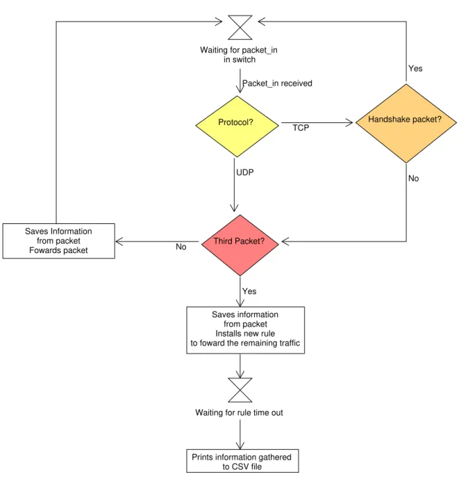
An OpenFlow application was created to: write rules in a switch, gather the firstN packets from each flow that comes to the switch, save the data gathered in a CSV file and be aware of the status of switches for the installation of proactive rules. In figure 3.4 we can see the flowchart of what happens to apacket_inthat enters in a switch, with our application.

(43)

3 . 4 . O P E N F L O W A P P L I C AT I O N

Prints information gathered to CSV file Waiting for rule time out

Waiting for packet_in in switch

Saves information from packet Installs new rule to foward the remaining traffic Saves Information from packet Fowards packet Third Packet? Handshake packet? Protocol? Yes Yes No Packet_in received No UDP TCP

Figure 3.4: Flowchart of the actions made by the OpenFlow application when apacket_in

is received in a switch

This application contains five classes that implement OpenFlow interfaces:

SwitchListener class implements an interface called DataPathListener, which

gives access to OpenFlow datapath events, such as the connect and disconnect of the switches. This class is responsible to install OpenFlow rules when the switch connects (proactive rules) and remove these rules when the switch disconnects.

PacketListener class implements an interface, called SequencePacketListener

which gives us access to the OpenFlow Packet-In message events meaning. If receives messages related to the existent traffic in the switch. This class filters the Packet-In received and is responsible to gather the firstN packets that come from each flow, which can be

(44)

either TCP or UDP.

IpPacketHandler creates one rule per flow that already had the first N packets saved. This rule is created so the packets from these flows wouldn’t go to the controller, proceeding as normal.

FlowEventListenerclass implements an interface, calledFlowEventListenerwhich gives information about flow-related events, such as when a flow is removed or modified.

DataStructureis the class responsible to store all the data gathered into a CSV file.

In the next subsections is presented a more detailed explanation about each class and their algorithm.

3.4.1 SwitchListener

SwitchListenerclass installs a total of five proactive rules in the switch, with the purpose of monitoring all TCP and UDP flows without interfering with other flows.

The first and second rules have the same priority and send all TCP and UDP traffic to table 200.

The third rule was created with an inferior priority to drop all traffic that wasn’t TCP or UDP. This rule would be used to forward the traffic as normal if we weren’t in the phase on gathering data with a mirror, this way the duplicate the packets from mirror are dropped.

The fourth and fifth rules send all TCP and UDP flows to the controller.

To write these five rules to tables were needed, table 100 and 200. Table 100 represents a Hardware which is a faster table, but only permits one rule with one instruction. Table 200 is a Software table, which makes it slower, but permits to create more than one instruction and more import it permits the gather of data from a flow when it ceases to exist. With the data obtained being Duration, Byte Count, number of packets this data. This information is used to label the flows according to their size and duration to help train the classifier. Once the classifier is trained table 200 won’t be needed and the process will be faster. Taking this into account, a total of five rules were created with three installed in table 100, and the other two in table 200.

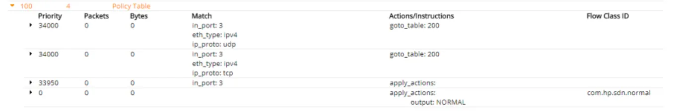
In 3.5 and 3.6 we can observe all five rules.

Figure 3.5: Rules installed in table 100

(45)

Figure 3.6: Rules installed in table 200

After carefully looking into figures 3.5 and 3.6 we can see that there are other rules besides the ones mention above. These are default rules. To counter these default rules, higher priority values were used in the rules created. Other information that we can gather from observing these images is that the match has as port of entry port 3 - this is where the traffic is coming from.

When the switch is disconnecting, this class removes the rules that were installed.

3.4.2 PacketListener

PacketListener class retrieves packets from either TCP or UDP flows. For TCP flows

the Flags of the TCP packet are analysed to exclude the initial handshake packets, more specifically the ones that contain the Synchronize (SYN) flag. This was realised since handshake packets don’t contain relevant data about the flow, since they are only used for synchronization.

We decided to use only three packets like was mention in the section 2.5.4 in previous chapter, since the results obtained with five packets were vastly similar to the ones with three packets so we saw no advantage in gather more packets. The gathering of more packets would increase the information that we could obtain making predictions more precise but it would come with the cost of a delay, since we would have to wait for all those packets to arrive. With less packets, the delay would be minor but we would have less information about the flow, which would decrease the accuracy of our classifiers. So a decision was made to only gather the first three packets.

In this class we restorted to Hashmaps to help us count the number of packets that came through the switch from each flow and also to save information such as size of packets and the arrival time. A total of three Hashmaps were used.

The first one is called Packets_per_flow and an entry is created when a new flow reaches the switch. The key used is a String composed by the source IP , the destination IP and the protocol (TCP or UDP). This key permits us to identify to which flow it belongs. The value is the number of the packets that have received, so we can know how many packets were gathered so far from each flow.

The other two Hashmaps arePacketsSizeandPacketsTime. Both use the same key as thePackets_per_flowHashmap but instead of a value they store an array. PacketsSize

stores an array with the size of each received packet andPacketsTimestores an array with the arrival time of each packet. The last position occupied in the array by data is given by

Packets_per_flowHashmap.

(46)

As we are getting the first three packets, these arrays are getting filled with their size and time of arrival. After receiving the third packet, a Flow Entry message is created to install in the switch a rule that matches packets from the flow, in method implemented inIpPacketHandler. Also at this time, all information gathered from the packet header (Date, Ethernet Type, source MAC address, source IP, destination IP, Protocol, source Port, destination Port) and both of the arrays (containing the size of first three packets and their arrival time) are sent to the classDataStructure, so the data can be saved in memory. A summary of this class is presented in figure 3.7 as a flowchart to facilitate the interpretation.

Third packet? Updates value in hashmap_{And saves the size} and arrival time by updating the hashmap Creates entry in hashmap

And saves the size and arrival time Check if it's

in hashmap Wait for Packet_in

FLAG SYN is active? Protocol?

Updates hashmaps with the size and arrival times Sends data to class DataStructure Calls method from IpPacketHandler

to install rule to foward packets Yes No Yes Yes No TCP UDP No

Figure 3.7: Flowchart of the class PacketListener

(47)

3.4.3 IpPacketHandler

IpPacketHandlerclass is used after gathering the three packets. It has the responsibility to create a new set of rules with higher priority than the ones created by theSwitchListener. The goal is to prevent that after the first initial three packets, subsequent packets of the same flow are no longer received in the controller.

Figure 3.8: Example of a TCP and UDP rule in table 200

In this figure 3.8 we can notice thatapply_action section is empty. This is because the rule was for gathering data, so the packet would be dropped. We don’t need those packets because of the mirror that was implemented.

3.4.4 FlowEventListener

FlowEventListener is used when the flow created by IpPacketHandler expires. This

means that the flow has stopped (there are no matching packets during theidle_timer

period). An OpenFlow message is sent by the switch that containsFlow_Entrystatistics, like information about the rest of the flow such as Duration, ByteCount and number of packets. This data is then sent to theDataStructureclass.

3.4.5 DataStructure

DataStructureis the class that creates a CSV file with all the data collected from the previous mentioned classes. After receiving the information from the first three packets, this data is stored in a structure. It is written in the CSV file after the rule of the flow expires. The information needed from the expiration of the flow is the total number of packets, the total duration and the total byte count. A cookie is used to coordinated the data received from the initial three packets and the statistics from the flow .

After this process, a line is written in the CSV file for the flow that contains: Date, Ether-net Type, source MAC address, source IP, destination IP, Protocol, source Port, destination Port, Cookie, Byte Count, Duration, Number of Packets, Reason for the flow to end (debug only), size of packet 1, size of packet 2, size of packet 3, and the difference between the arrival times between three packets (Interval1 =ArrivalT imeP3−ArrivalT imeP2and

(48)

Figure 3.9: Example of two flows saved in the csv file

3.5 Python Script

A tool was needed to implement the classifier, and two options that had the requirements that we needed were available: Python and R. Python was chosen because I was more familiarized with it and have work with it in the past. Both of them are open source and have a variety of extremes packages available to use. A similar implementation with R would give the same results, it was just the preference to use Python.

An extensive list of packages from the sklearn library were used to implement each classifier and for the separation of the data, in the training set and the test set. As the name suggests, the training set its a portion of the data used to train the classifier. The test set is the remaining data and it is used to evaluate the classifier in terms of performance and validation of the classification made.

Other packages used were numpy and pandas. They were used to manipulated the data from the CSV. Another library used was matplotlib, to represent data in graphics.

In this script we started by reading the CSV created by our OpenFlow aplication with all of our gathered data. Then we modified the values that weren’t float values, such as the type of Protocol, source IP, destination IP, source Port, destination Port. For example, since there were only two protocols that we were interested, TCP was converted to 1 and UDP to -1. This was very important since the majority of the classifiers used only accept data in the format of a number.

Then we had to label all the flows from our data so the classifier could predict it. In this project two types of classification were conducted: one by size of the flow, and the other by its duration. The first consisted in predicting the total size of the designated flow and the second consisted in predicting its duration.

(49)

3 . 5 . P Y T H O N S C R I P T

Figure 3.10: Histogram of the size of the flows

In figure 3.10 we can observe the distribution of the sizes of the packets gathered. This histogram was used to label the data regarding their size. At first we started to divide in five equally distributed classes but the precision results obtained were very low, around 60%. So we decided to diminish the number of classes. After trying several thresholds and different number of classes we ended up with three classes with the thresholds mention in table 3.1. These were the ones that gave us the results in 4.3. Better results were achieved with only two classes with a difference of 2% in the average scores, but we decided to use three classes since the difference was small. This permitted a distinction between packets over 1000 bytes but under 2500 bytes.

Table 3.1: Classes for Size Classification

Size (bytes) Class

x< 1000 0 1000 < x< 2500 1

x> 2500 2

Regarding the duration classification, the same method was applied but it was more problematic since the majority (87% of the data gathered) of the durations were short (under 5 seconds), creating a big difference between the rest of the flows. This was due to most of the traffic gathered being "short lived" such as logins, reaching and loading web-sites. In this classification only two classes were used. The thresholds used are mentioned in table 3.2.

Table 3.2: Classes for Duration Classification

Duration (seconds) Class

x< 5 0

x> 5 1

After all data is converted a normalization was made to achieved a faster index search-ing and faster data modifications, decreassearch-ing the time that was needed to train and test

(50)

the classifiers. Also this way the results obtained from the classifiers wouldn’t be affected by the distribution of data, since we now had a normal distribution.

We then separate all data in two distinct sets: the training data and the test data with the ratio67/33(training/test). This ratio was chosen because is the most commonly used in the machine learning [19]. These ratio tries to find a balance between the two sets. If we increase the percentage of the training data too much the classifier could suffer from overfitting which would mean the the classifier didn’t learn but memorized the answers for this data. On the other hand, increasing the percentage of the test data the performance of the controller could be reduced since it had less example to practice, causing underfitting.

We proceed to train each classifier with the train set. After the training of each clas-sifier, we would perform a test with a cross validation table. Several parameter were altered in each classifier to obtain better results considering our data. These results and configurations can been seen in section 4.3.

(51)

C

H

A

P

T

E

R

4

R

E S U L T S

4.1 Introduction

In this chapter we start with a brief explanation about True Positives, True Negatives, False Positives and False Negatives values. Then classifier evaluation metrics such as Accuracy, Precision, Recall and F1 score are introduced. Finally the most important results of the five used classifiers used (Random Forest, Neural Networks with Multi-layer Perceptron and K-Neighbour) are presented. The configurations used in each classifier and their impact on performance are also discussed.

4.2 Classification metrics

Considering a binary classifier, that can classify between class 0 and class 1, with class 0 representing a positive (exists) and class 1 a negative (doesn’t exist). We can use the following terminologies:

True Positives (TP) are the correctly predicted positive values, which means that the actual value is 0 and the predicted value is also 0. E.g. A flow belongs to class 0 and the prediction also predicts that the flow belongs to class 0.

True Negatives (TN) are the correctly predicted negative values which means that the actual value is 1 and the value of predicted class is also 1.

False positives and false negatives occur when the prediction contradicts with the actual class.

False Positives (FP) is when the real class is 1 and the predicted class is 0.

False Negatives (FN) is when the real class is 0 but the predicted class in 1.