Lat. Am. j. solids struct. vol.12 número9

(1)

Abstract

The understanding of phenomena, no matter their nature is based on the experimental results found. In the most cases, this requires an important number of tests in order to put a reliable and useful observation served into solving the technical problems subsequent-ly. This paper is based on independent and variables combination resulting from experimentation in a mathematical formulation. Indeed, mathematical modeling gives us the advantage to optimize and predict the right choices without passing each case by the experiment. In this work we plan to apply the experimental design method on the experimental results found by Deokar, A (2011), concerning the effect of the size and position of a crack on the measured frequency of a beam console, and validating the mathe-matical model to predict other frequencies

Keywords

Parameters, experimental design method, modeling, frequency, crack.

Modeling of Cracked Beams by the Experimental Design Method

1 INTRODUCTION

Several scientific works has been conducted on the experimental design method each in its field of

application and its objective, Bounazef M, Goupy J and Castro. L (2009, 1925, 2004). Other

au-thors Aît Yala (2009) have implemented experimental design using numerical results.

Experi-mental design were used for the first time by Fisher R (1925), in the field of agriculture where the

experimental parameters are numerous and significant which leads to mathematical modeling and

therefore to optimize the model sought. In mechanical terms, for example, Serier et al (2013a)

used experimental design method for optimizing the machining parameters in order to increase

the life of the tool. These same authors (2013b) performed a work in the field of vibration where

they showed the importance of the geometrical properties, the speed of rotation of a shaft (tree)

on the opening and closing mechanism of crack in a rotating machine. It is clear that the

phe-nomenon of cracking beams has negative consequences on the large industrial constructions,

Thomas, M (1995). The work of Deokar, A (2011) has focused on the experimental investigation

M. Serier a N. Benamara a A. Megueni a K. Refassi a

a _{Mechanics of Structures and Solids}

Laboratory. Faculty of Technolgy, University of Sidi-Bel-Abbes, Bp 89, cité Ben M’hidi sidi- Bel-Abbes 22000-Algeria

http://dx.doi.org/10.1590/1679-78251403

(2)

Latin A m erican Journal of Solids and Structures 12 (2015) 1641-1652

for the detection of a crack on a cantilever used a criteria based on natural frequencies. Our work

consisted on the use of experimental design method for modeling and prediction of frequencies.

2 EXPERIMENTAL RESULTS FOR EACH FREQUENCY MODE

In the tables below, the experimental results of the variation of frequency ratio as a function of

position and depth of modes 1, 2 and 3 are presented. These results came from the work of Deokar

(2011).

Physical values of parameters Coded values of parameters Experimental results

N Crack

depth

Crack location

Frequency

ratio first mode a0 X1 X2 I12 y

01 2 25 0,9887 1 -1 -1 1 0,9887

02 2 100 0,9956 1 -1 -0,14 0,14 0,9956

03 2 200 0,9996 1 -1 +1 -1 0,9996

04 6 25 0,91 1 -0,2 -1 0,2 0,91

05 6 100 0,9626 1 -0,2 -0,14 0,028 0,9626

06 6 200 0,9966 1 -0,2 +1 -0,2 0,9966

07 12 25 0,6465 1 +1 -1 -12 0,6465

08 12 100 0,8081 1 +1 -0,14 -1,68 0,8081

09 12 200 0,9766 1 +1 +1 12 0,9766

Table 1: Frequency ratio of the various tests of the first mode and experience matrix.

Table 2: Frequency ratio of the various tests of the second mode and experience matrix.

Physical values of parameters Coded values of parameters Experimental results

N Crack depth

Crack location

Frequency ratio

second mode a0 X1 X2 I12 y

01 2 25 0,9951 1 -1 -1 1 0,9951

02 2 100 0,9975 1 -1 -0,14 0,14 0,9975

03 2 200 0,995 1 -1 +1 -1 0,995

04 6 25 0,9641 1 -0,2 -1 0,2 0,9641

05 6 100 0,9663 1 -0,2 -0,14 0,028 0,9663

06 6 200 0,9316 1 -0,2 +1 -0,2 0,9316

07 12 25 0,8903 1 +1 -1 -12 0,8903

08 12 100 0,9039 1 +1 -0,14 -1,68 0,9039

(3)

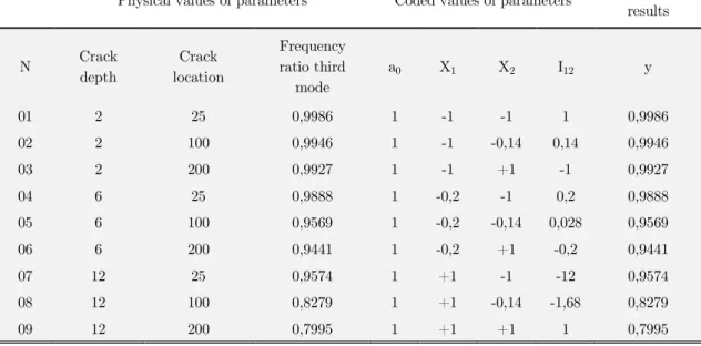
Latin A m erican Journal of Solids and Structures 12 (2015) 1641-1652 Physical values of parameters Coded values of parameters Experimental

results

N Crack

depth

Crack location

Frequency ratio third

mode

a0 X1 X2 I12 y

01 2 25 0,9986 1 -1 -1 1 0,9986

02 2 100 0,9946 1 -1 -0,14 0,14 0,9946

03 2 200 0,9927 1 -1 +1 -1 0,9927

04 6 25 0,9888 1 -0,2 -1 0,2 0,9888

05 6 100 0,9569 1 -0,2 -0,14 0,028 0,9569

06 6 200 0,9441 1 -0,2 +1 -0,2 0,9441

07 12 25 0,9574 1 +1 -1 -12 0,9574

08 12 100 0,8279 1 +1 -0,14 -1,68 0,8279

09 12 200 0,7995 1 +1 +1 1 0,7995

Table 3: Frequency ratio of the various tests of the third mode and experience matrix.

3 CALCULATIONS OF THE EFFECTS OF FACTORS

Each factor xi is affected (acted on) the behavior of the beam and it’s defined by the effect of

a

i

. It

is possible that the factors interact with each other, this is the case in our work, and therefore we

are left with three factors, instead of two, including the average of these latter. In other words any

response

y

i

depends on the action of all factors together xi. Analytically, and the relationship

be-tween the response factor can exist only when a certain proportionality exists bebe-tween them. This

leads us to write

:

 n1  np  p1

y



x



a

(1)

The Solve of system of equations is based on the least squares method, and the solution is noted a.

This solution is given by the following formula derived from the theory of matrix calculation.

(2)

Therefore

Coefficients Mode 1 Mode 2 Mode3

0,92 0,93 0,93

-0,090 -0,070 -0,070

0,076 -0,026 -0,036

0,081 -0,028 -0,037

(4)

The models are thus written in the following forms

Mode 1:

y₁



0.92 

0.090  

X₁



0.076  

X₂



0.081 

X X₁ ₂



Mode 2:

y₂



0.93 

0.070  

X₁



0.026  

X₂



0.028 

X X₁ ₂



Mode 3:

y

₃



0.93 

0.070  

X

₁



0.036  

X

₂



0.037 

X X

₁ ₂



4 ANALYSES WITH ONE VARIABLE FACTOR

4.1 Effect of Each Factor for the Three Modes

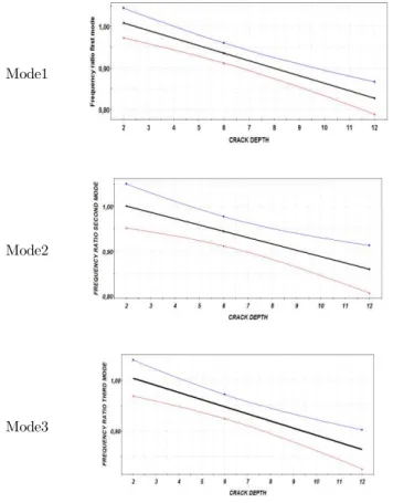
The figures below represent the effect of the two most principals factors (the crack depth and

posi-tion of the crack) for each mode of vibraposi-tion. We note that the ratio of the frequency is proporposi-tion-

proportion-al to the crack depth; the slope is negative regardless of the active mode. This confirms that the

propagation of a crack causes a decrease in the ratio of the frequency. In the case of the effect of

crack position on the frequency, we observed a change of the upward frequency in the first mode. In

other words, the more crack is remote from the recess the more important is the frequency, however

in the case of other modes (2 and 3) an opposite change is noticed with slopes more or less

im-portant. This is due to the values of the amplitudes of modes 2 and 3.

Mode1

Mode2

Mode3

Figure 1: Effect of the depth of the crack on the frequency for the three modes.

(5)

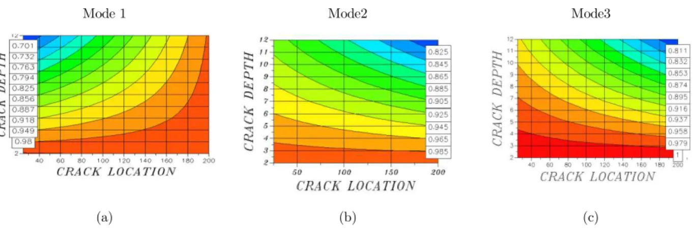
5 INTERACTION ANALYSE

Mode 1 Mode2 Mode3

(a) (b) (c)

Figure 3: Effect of the interaction of two factors on the frequencies for the three modes.

The analyze of the interaction between the depth and crack location was done by the help of a

rep-resentation of iso-courbes

Mode 1 Crack depth (2mm) Crack depth(12mm)

Crack location (25mm) 0,98 0,701

Table 5: The results of combined effects (mode1).

The figure 3a represents the effects of the two factors versus the ratio of frequency in mode 1. We

observed that there is just one near the abscissa of embedding and at low depths frequency ratio

reached the value of 0.98. This ratio decreases to great depths. For abscissa near the edge of the

beam, the depth of the crack has not effect. In the second and third mode analysis of iso-curves

(fig.3b, 3c) shows that the ratio reaches its maximum when the two factors are the lowest values

(tableaux 6 and 7)

Table 6: The results of combined effects (mode 2).

(6)

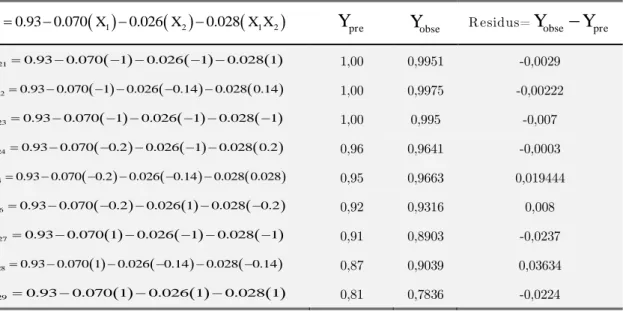
6 ANALYZE WITH THREE FACTORS

The mathematic models already established, they allowed us to calculate the predicted frequencies

and the residues for each mode (table 8, 9 and 10).

 





1 0.92 0.090 1 0.076 2 0.081 1 2

y   X  X  X X

Y

_pre

obse

Y

R esidus=

Y

_obse



Y

_pre

 

11 0.92 0.090 1 0.076 1 0.081 1

y      

 









12 0.92 0.090 1 0.076 0.14 0.081 0.14

y      

1,02 1,01 0,9887 0,9956 -0,0263 -0,0151

 

13 0.92 0.090 1 0.076 1 0.081 1

y       _1,01 _0,9996 _-0,0054





 





14 0.92 0.090 0.2 0.076 1 0.081 0.2

y       _0,88 _0,91 _0,0318













15 0.92 0.090 0.2 0.076 0.14 0.081 0.028

y       _0,93 _0,9626 _0,032972





 





16 0.92 0.090 0.2 0.076 1 0.081 0.2

y       _1,00 _0,9966 _-0,0012

 

17 0.92 0.090 1 0.076 1 0.081 1

y       _0,67 _0,6465 _-0,0265

 









18 0.92 0.090 1 0.076 0.14 0.081 0.14

y       _0,80 _0,8081 _0,0081

 

19 0.92 0.090 1 0.076 1 0.081 1

y     _0,99 _0,9766 _-0,0104

Table 8: Residues for the mode 1.

 





2 0.93 0.070 1 0.026 2 0.028 1 2

y   X  X  X X

Y

_pre

Y

_obse R esidus=

Y

_obse



Y

_pre

     

21 0.93 0.070 1 0.026 1 0.028 1

y       _1,00 _0,9951 _-0,0029

     

22 0.93 0.070 1 0.026 0.14 0.028 0.14

y       _1,00 _0,9975 _-0,00222

     

23 0.93 0.070 1 0.026 1 0.028 1

y        _1,00 _0,995 _-0,007

     

24 0.93 0.070 0.2 0.026 1 0.028 0.2

y       _0,96 _0,9641 _-0,0003

     

25 0.93 0.070 0.2 0.026 0.14 0.028 0.028

y       _0,95 _0,9663 _0,019444

     

26 0.93 0.070 0.2 0.026 1 0.028 0.2

y       _0,92 _0,9316 _0,008

     

27 0.93 0.070 1 0.026 1 0.028 1

y       0,91 0,8903 -0,0237

     

28 0.93 0.070 1 0.026 0.14 0.028 0.14

y       0,87 0,9039 0,03634

     

29 0.93 0.070 1 0.026 1 0.028 1

y     0,81 0,7836 -0,0224

(7)

 





3

0.93 0.070

1

0.036

2

0.037

1 2

y





X



X



X X

Y

_pre

Y

_obse Residus =

Y

_obse



Y

_pre

 

31 0.93 0.070 1 0.036 1 0.037 1

y       _1,00 _0,9986 _-0,0004

 









32 0.93 0.070 1 0.036 0.14 0.037 0.14

y       _1,00 _0,9946 _-0,00526

 

33 0.93 0.070 1 0.036 1 0.037 1

y       _1,00 _0,9927 _-0,0083





 

34 0.93 0.070 0.2 0.036 1 0.037 0.2

y       _0,97 _0,9888 _0,0162













35 0.93 0.070 0.2 0.036 0.14 0.037 0.028

y       _0,95 _0,9569 _0,008896





 





36 0.93 0.070 0.2 0.036 1 0.037 0.2

y       _0,92 _0,9441 _0,0287

 

37 0.93 0.070 1 0.036 1 0.037 1

y       _0,93 _0,9574 _0,0244

 









38 0.93 0.070 1 0.036 0.14 0.037 0.14

y       _0,87 _0,8279 _-0,04232

 

39 0.93 0.070 1 0.036 1 0.037 1

y     _0,79 _0,7995 _0,0125

Table 10: Residues for the mode 3.

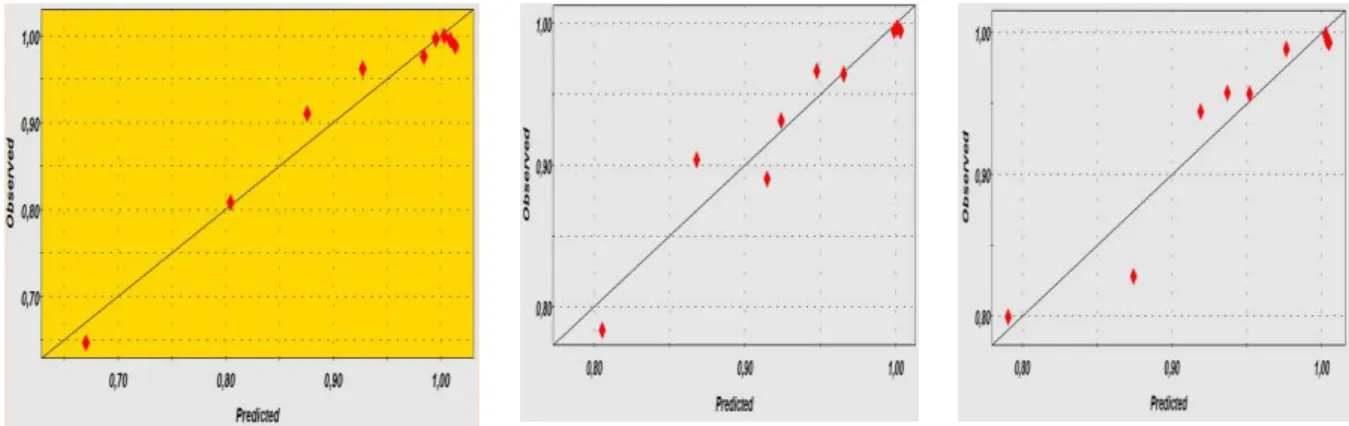
With the help of the statistics calculations, we were able to define the effects the most significant of

the factors and their gaps of confidence (trust), all with calculating the residues ei. The residues are

the difference between the experimental value and predicted value by the mathematic model

(fig-ure4) and they are linked by the linear regression.

Figure 4: Distribution of the experimental points from the mathematical model for each mode.

7 REALIZATION OF THE TEST OF EFFECTS SIGNIFICANCE

The test used is the Student test << t>>. An effect is said significant (that is to say that the

in-teraction or the variable associated with it has an influence on the response), if, for a given risk

significantly different from 0. So we test the hypothesis

Hypothesis:

(8)

For this, we calculate

i i i

a

t

s



(3)

Student table is then used to v= n

–

p degrees of freedom (n is the number of experiments and p is

the number of effects including the constant). The risk of a first species is selected (usually 1% or

5%) and is read in the table of the Student t value, using the part of the table related to a bilateral

test.

Mode 1:

2

1

2

i

s e

n p







(4)



 





 



2 2 2 2 2 2

2

2 2 2

1

0.0263 0.0151 0.0054 0.0318 0.032972 0.0012

9 4

0.0265 0.0081 0.0104

s          

      







2

1 0.0039

5

s







2

0.00078

s



The variance calculated for each effect is then:





2

1 0.00078

9

s



2

0.000086

s



0.0093

i s



 

0.01 1%

4.032

9

4

5

ti





 



_{ }

   



(5)

Therefore:

ti

 

si

0.037 The effect of crack depth :

The effect of crack location

The effect of general average

The effect of the interaction :

│

-0.09

0│> 0.03

7 significatif

│

+0.92

0│> 0.03

7 significatif

│

-0.810

│< 0.03

7 significatif

(9)

Confidence interval of model effects of the first mode

[a

i

- t (

α

,

ν

) s

i

; a

i

+ t (

α

,

ν

) s

i

]

(6)

ai-(t(α,ν) *si) ai ai+ (t (α,ν) *si)

-0,127 C

rack depth

-0,09 -0,053

0,039

_{Crack location}

0,076 0,113

0,044 Interaction 0,081 0,118

Table 11: Confidence interval of model effects of the first mode.

Figure 5: Confidence interval of model effects of the first mode.

Mode

2:

2

1

2

i

s e

n p









 





 



2 2 2 2 2 2

2

2 2 2

1

0.000008 0.000004 0.00004 0.00000009 0.0003 0.00006

9 4

0.0005 0.0013 0.0005

s          



     







2

1 0.0028

5

s







2

0.00057

s



The variance calculated for each effect is then:





2

1 0.00057

9

s



2

0.000060

(10)

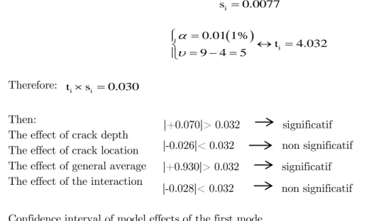
0.0077

i

s



 

0.01 1%

4.032

9

4

5

ti





 



_{ }

   



Therefore:

t_i

 

s_i

0.030 Then:

The effect of crack depth :

The effect of crack location :

The effect of general average :

The effect of the interaction :

Confidence interval of model effects of the first mode

[a

i

- t (

α

,

ν

) s

i

; a

i

+ t (

α

,

ν

) s

i

]

ai-(t(α,ν) *si) ai ai + (t (α,ν) *si)

-0,098 Crack depth -0,07 -0,038

-0,05824 Crack location -0,026 0,006

-0,06024 Interaction -0,028 0,004

Table 12: Confidence interval of model effects of the second mode.

Figure 6: confidence interval of model effects of the second mode.

Mode 3:

2

1

2

i

s e

n p









 





 



2 2 2 2 2 2

2

2 2 2

1

0.0004 0.00002 0.000068 0.00026 0.00007 0.00082

9 4

0.00059 0.0017 0.00015

s          



     



│

+

0.070│> 0.032

significatif

│

+

0.930│> 0.032

significatif

│

-0.028

│< 0.032

non significatif

(11)





2

1 0.0038

5

s







2

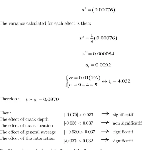
0.00076

s



The variance calculated for each effect is then:





2

1 0.00076

9

s



2

0.000084

s



0.0092

i

s



 

0.01 1%

4.032

9

4

5

ti





 



_{ }

   



Therefore:

ti

 

si

0.0370

Then:

The effect of crack depth :

The effect of crack location :

The effect of general average :

The effect of the interaction :

Confidence interval of model effects of the first mode

[a

i

- t (

α

,

ν

) s

i

; a

i

+ t (

α

,

ν

) s

i

]

ai -(t(α,ν) *si)

ai ai + (t (α,ν) *si)

-0,107 Crack depth -0,07 -0,033

-0,073 Crack location -0,036 0,001

-0,074 Crack depth -0,037 0

Table 13: Confidence interval of model effects of the third mode.

│

-

0.070│> 0.03

7 significatif

│

+

0.930│> 0.03

7 significatif

│

-0.0

37│>

0.032 significatif

(12)

Figure 7: Confidence interval of model effects of the third mode.

8 CONCLUSIONS

Using the method of experimental design allows to extract the maximum information at a

reasona-ble cost and minimum time. In our case, we have:

1) Modeled the vibration behavior of a cracked beam console

2) Plotted the iso-curves for different modes of vibration

These curves allow the choice according to the needs of the operating state (condition) of the beam.

It further notes that:

The depth of the crack remains significantly regardless of the current mode vibration, while this is

not the case for the location of the crack which is significant only in the first mode.

The interaction between the two factors of an unexplained way varies from one mode to another; in

the first mode of interaction is significant, it is only slightly in the third mode when it no longer is

in the second mode

References

Deokar, A. A.V, Wakchaure,B. V.D. (2011). Experimental Investigation of Crack Detection in Cantilever Beam Using Natural Frequency as Basic Criterion, INSTITUTE OF TECHNOLOGY, NIRMA UNIVERSITY, AHMEDABAD – 382 481

Bounazef ,M., Djeffal ,A., Serier ,M.and Adda ,BEA. (2009). Optimization by behavior modeling of a protective porous material. Journal of the Computational Materials Science. 44(3):921-928.

Fisher,R. (1925). Statistical Methods for Research Workers. Oliver and Boyd;. PMid: 17246289 Castro.L, Viéville.P, and Lipinski.P, Phys. J(2006).IV France 134, 1273.

A. Ait Yala , A. Megueni, (2009) Optimisation of composite patches repairs with the design of experiments method, Mate-rials and Design pp 200–205

Thomas, M., Nguyen, H., Hamidi,L., Massoud ,M. and Piaud J.B. (1995). Detection of rotor cracks by experi-mental modal analysis, Transactions of the Canadian Society of Mechanical Engineering, 19(2): pp 155-174.

Refassi,K. Serier, M. and Lousdad ,A. (2013). DOE Analysis of Feed and Cutting Speed Effects on Frequency Dur-ing MachinDur-ing Operations, Advanced Science Letters Vol. 19, 942–945.