EXPERIMENTAL STUDY OF PROTON INDUCED NUCLEAR REACTIONS IN6,7 Li

EXPERIMENTAL STUDY OF PROTON

INDUCED NUCLEAR REACTIONS IN

Li

Disserta¸c˜

ao apresentada para

obten¸c˜

ao do grau de Doutor em F´ısica,

especialidade de F´ısica Nuclear,

pela Universidade Nova de Lisboa,

Faculdade de Ciˆ

encias e Tecnologia.

This work has been done in a framework of an international collaboration and, in spite of the long list of people, I wish to thank all of them for their help. My special thanks go to:

Professor Adelaide Pedro de Jesus, who gave me the opportunity to join the Lisboa group, introducing me to the exciting field of nuclear astrophysics. Her constant support during all the phases of my work is gratefully acknowledged.

Professor Claus Rolfs, for his guidance and constant support during my stays at Bochum. Prof. Dr. Jo˜ao Pires Ribeiro, for his support during data taking, and electronics and physics teachings.

Prof. Dr. Rui Coelho da Silva, who contributed to this work with very interesting discus-sions about physics.

Dr. Rodrigo Mateus, Eng. Micaela Fonseca and Eng. H´elio Lu´ıs, for their friendship and constant support during the long runs of data taking.

Dr. Francesco Raiola, for his friendship and fruitful discussions about electron screening (and airplanes).

Dr. Karl Kettner, for his big help in spectra analysis.

Dr. Eduardo Alves, for his teachings in physics and on the Van de Graaffaccelerator opera-tion techniques.

Manuel Cabac¸a for converting on the lathe, my blueprints into pieces for the target chamber, and for his valuable help in mechanical issues.

Jorge Rocha for doing the lithium implantations and for helping with his expertise in vacuum technology.

Eng. Hugo Marques and Prof. Dr. Orlando Teodoro for taking the SIMS and XPS spectra and helping me in the analysis.

Este trabalho apresenta os resultados do estudo experimental das reacc¸ ˜oes nucleares induzi-das por prot˜oes em l´ıtio, nomeadamente as reacc¸ ˜oes 7_Li(p,α)4_He,6_Li(p,α)3_{He e}7_Li(p,p)7_Li.

As abundˆancias de7_{Li e}6_{Li identificadas como primordiais e observadas em estrelas muito}

antigas do halo da Via L´actea diferem consideravelmente dos valores previstos por mode-los de nucleoss´ıntese primordial e evoluc¸˜ao estelar que dependem, entre outros factores, das secc¸˜oes eficazes de reacc¸ ˜oes nucleares como a7_Li(p,α)4_{He e a}6_Li(p,α)3_{He. A procura da}

res-posta para estas discrepˆancias desencadeou nestes ´ultimos anos investigac¸˜ao intensa nos campos da evoluc¸˜ao estelar, da cosmologia, da evoluc¸˜ao pr´e-gal´actica e das reacc¸ ˜oes nucleares a baixa energia.

Focando-se nas reacc¸ ˜oes nucleares, este trabalho determinou com maior precis˜ao experi-mental as secc¸˜oes eficazes (expressas em termos do factor astrof´ısico) das reacc¸˜oes7_Li(p,α)4_He

e 6_Li(p,α)3_{He e os efeitos de blindagem electr´onica nestas reacc¸˜oes para diferentes}

ambi-entes (alvos isolantes e met´alicos). Foram igualmente medidas as distribuic¸˜oes angulares da reacc¸˜ao do7_{Li. Estas medic¸˜oes foram realizadas em dois laborat´orios, no ˆambito da colaborac¸˜ao}

internacional LUNA (Laboratory for Undergroud Nuclear Astrophysics), nomeadamente o La-borat´orio de Feixe de I˜oes do ITN (Instituto Tecnol´ogico e Nuclear) em Sacav´em, Portugal e o Dynamitron-Tandem-Laboratorium na Ruhr-Universit¨at em Bochum, Alemanha. No ITN, a cˆamara dos alvos foi modificada de forma a optimizar a medic¸˜ao destas reacc¸˜oes com o de-senho e construc¸˜ao de novas pec¸as, a inclus˜ao de mais uma bomba turbomolecular no sistema e de um dedo frio. As reacc¸ ˜oes7_Li(p,α)4_{He e}6_Li(p,α)3_{He foram medidas em simultˆaneo com}

sete e quatro alvos, respectivamente. Os alvos foram produzidos de forma a obter perfis de l´ıtio em profundidade adequados e est´aveis.

de Debye aplicado aos electr˜oes de conduc¸˜ao dos metais consegue reproduzir estes valores cons-tituindo um modelo simples, mas que parametriza com robustez os dados experimentais. Ao n´ıvel dos modelos estelares e de nucleoss´ıntese primordial, estes resultados s˜ao muito impor-tantes porque mostram que as medic¸˜oes em laborat´orio est˜ao bem compreendidas e, portanto, os parˆametros de entrada destes modelos correspondentes `as secc¸˜oes eficazes est˜ao correctos.

Neste trabalho tamb´em foi medida a secc¸˜ao eficaz diferencial da reacc¸˜ao de dispers˜ao el´astica dos prot˜oes por7_{Li, ´util para descrever o canal de entrada da reacc¸˜ao}7_Li(p,α)4_He.

Palavras chave

This work presents the results of the experimental study of proton induced nuclear reactions in lithium, namely the7_Li(p,α)4_He,6_Li(p,α)3_{He and}7_Li(p,p)7_{Li reactions.}

The amount of 7_{Li and} 6_{Li identified as primordial and observed in very old stars of the}

Milky Way galactic halo strongly deviates from the predictions of primordial nucleosynthesis and stellar evolution models which depend, among other factors, on the cross sections of re-actions like7_Li(p,α)4_{He and} 6_Li(p,α)3_{He. These discrepancies have triggered a large amount}

of research in the fields of stellar evolution, cosmology, pre-galactic evolution and low energy nuclear reactions.

Focusing on nuclear reactions, this work has measured the7_Li(p,α)4_{He and}6_Li(p,α)3_He

re-actions cross sections (expressed in terms of the astrophysicalS-factor) with higher accuracy, and the electron screening effects in these reactions for different environments (insulators and metallic targets). The7_Li(p,α)4_{He angular distributions were also measured. These}

measure-ments took place in two laboratory facilities, in the framework of the LUNA (Laboratory for Un-dergroud Nuclear Astrophysics) international collaboration, namely the Laborat´orio de Feixe de I˜oes in ITN (Instituto Tecnol´ogico e Nuclear) Sacav´em, Portugal, and the Dynamitron-Tandem-Laboratorium in Ruhr-Universit¨at Bochum, Germany. The ITN target chamber was modified to measure these nuclear reactions, with the design and construction of new components, the addition of one turbomolecular pump and a cold finger. The7_Li(p,α)4_{He and}6_Li(p,α)3_He

reac-tions were measured concurrently with seven and four targets, respectively. These targets were produced in order to obtain adequate and stable lithium depth profiles.

results are very important as they show that laboratory measurements are well controlled, and the model inputs from these cross sections are therefore correct.

In this work the7_Li(p,p)7_{Li differential cross section was also measured, which is useful to}

describe the7_Li(p,α)4_{He entrance channel.}

Keywords

Primordial lithium, charged-particle-induced nuclear reactions, cross section, Astrophysical

A Abundance A Mass number

Aℓ Angular distribution coefficient

B Magnetic induction

c Speed of light

dσ/dΩ Differential cross section

DN Nominal fluence

DI Retained fluence

E Center-of-mass reference frame energy

Elab Laboratory reference frame energy

EC Coulomb barrier

EG Gamow energy

E0 Gamow peak maximum

E0 Incident energy

Er Resonance energy

f Screening factor

fp Screening factor in a plasma

F Effective area for collision

g Surface gravity

H Hubble constant

h Planck constant

ℏ _{Reduced Planck constant}

~_{j Particle spin} ~

J Total angular momentum

J Bessel function

J Flux of incident particles

k Thermal conductivity

k Wavenumber

kB Boltzmann constant

K_Ω Solid angle transformation between the laboratory and center-of-mass frame

~ℓ Orbital angular momentum

m Mass

N Number of particles

N Areal density (number of particles per square centimeter)

NA Avogadro number

Np Number of incident protons

n Atomic density (number of particles per cubic centimeter)

ne Conduction electrons density

ne0 Conduction electrons average density

ne f f Number of conduction electrons per metallic atom

~

p Linear momentum P Pressure

P Power

Pℓ Legendre polynomial qe Electron electric charge

Q ReactionQ-value

Q Electric charge

Qℓ Solid angle correction factor r Stoichiometric ratio

r Total reaction rate

~r Position

Rc Classical turning point

RD Debye-H¨uckel radius/Debye radius

RH Bohr radius

Rn Nuclear radius

RHall Hall coefficient

Rp Projected range

S Sputtering yield

S AstrophysicalS-factor

Seff Effective astrophysicalS-factor

T Absolute temperature

T6 Absolute temperature in millions of K

T9 Absolute temperature in billions of K

Teff Star’s effective absolute temperature

UD Debye energy

Ue Electron screening potential energy

Ueexp Experimental electron screening potential energy

Uth

e Theoretical electron screening potential energy

U_esud Uesudden limit

Uad

e Ueadiabatic limit

U_ebound Bound electron screening potential energy

~v Velocity

V Potential energy

W Angular distribution

x Depth

X Mass fraction

Vc Coulomb potential energy

y Solubility

Y Reaction yield per incident particle

Yp 4He primordial abundance

Z Atomic number

Γ Resonance width

δ Kronecker delta

δ Uncertainity

∆ Target thickness

∆ Energy step

∆Rp Straggling

ǫ Stopping power cross section

ǫ0 Permittivity of free space

ǫeff Effective stopping power cross section η Baryon-to-photon ratio

η Sommerfeld parameter

η Si detector efficiency

θ Scattering angle in center-of-mass frame

θlab Scattering angle in laboratory frame n _{Reduced de Broglie wavelength} µ Reduced mass

ξ Microturbulence

φ Probability function

φ Coulomb potential

ρ Density

ρa Atomic density

π Parity

σ Cross section

σ Depletion

σ Standard deviation

σb Bare nucleus cross section

σs Screened nucleus cross section

σp Screened nucleus cross section in a plasma

< σv> reaction rate per particle pair

Ω_lab Solid angle in laboratory frame

ADC Analog-to-Digital Converter AMRSFs Average Matrix Sensitive Factors BBN Big Bang Nucleosynthesis CAB Cores and Bonds

CeFITec Centro de F´ısica e Investigac¸˜ao Tecnol´ogica CMB Cosmic Microwave Background

DTL Dynamitron-Tandem-Laboratorium FWHM Full Width at Half Maximum GIDS Grupo de I & D em Superf´ıcies GCR Galactic Cosmic Rays

GUI Graphics User Interface ISM Interstellar Medium

ITN Instituto Tecnol´ogico e Nuclear LTE Local Thermodynamic Equilibrium

LUNA Laboratory for Underground Nuclear Astrophysics MB Maxwell-Boltzmann

NASA National Aeronautics and Space Administration ndf number of degrees of freedom

PIGE Proton Induced Gamma-ray Emission PIPS Passivated Implanted Planar Silicon RBS Rutherford Backscattering Spectroscopy RGB Red Giant Branch

SIMS Secondary Ion Mass Spectrometry SN Supernovae

THM Trojan-Horse Method

Introduction 1

1 Primordial lithium in the universe 5

1.1 Big Bang Nucleosynthesis . . . 6

1.1.1 SBBN primordial abundances compared to observations . . . 8

1.2 Search for solutions to the lithium discrepancies . . . 18

1.2.1 Stellar . . . 19

1.2.2 Pre-galactic evolution . . . 23

1.2.3 Cosmology . . . 26

1.2.4 Nuclear . . . 27

2 Determination of nuclear reaction rates 31 2.1 Nuclear reaction rate . . . 31

2.2 Coulomb barrier and Gamow peak . . . 33

2.3 Electron screening . . . 36

2.3.1 Theoretical models . . . 39

2.3.2 Electron screening in D(d,p)T . . . 41

3 Available data on the7Li(p,α)4He and6Li(p,α)3He reactions 45 3.1 Methods for fitting data . . . 45

3.1.1 S-factor . . . 45

3.1.2 Angular distributions . . . 47

3.2 Fits to7_Li(p,α)4_{He data . . . . 50}

3.2.2 Angular distributions . . . 56

3.3 Fits to6_Li(p,α)3_{He data . . . . 56}

3.3.1 S-factor . . . 56

3.3.2 Angular distributions . . . 60

4 Experimental details 61 4.1 Experimental setup . . . 61

4.1.1 ITN setup . . . 62

4.1.2 DTL setup . . . 69

4.2 Target preparation and analysis . . . 72

4.2.1 LiF targets . . . 72

4.2.2 7_{Li implanted into Al target . . . . 79}

4.2.3 PdLix targets . . . 91

4.2.4 Li metal target . . . 92

4.2.5 Li2WO4target . . . 93

4.2.6 Targets stability . . . 94

5 Analysis and results 97 5.1 S-factor determination . . . 97

5.1.1 Integral method . . . 97

5.1.2 Differential method . . . 98

5.1.3 Effective stopping cross section . . . 100

5.1.4 Solid angle transformation between the laboratory and center of mass systems . . . 102

5.1.5 Angular distributions . . . 103

5.1.6 Error analysis . . . 108

5.2 Results forSb(E) andUe . . . 114

5.2.1 Integral method –Sb(E) . . . 114

5.2.2 Differential method –Ue . . . 130

5.3 Debye shielding . . . 134

5.3.1 Electron screening in the Li2WO4insulator . . . 136

5.3.3 Electron screening in the PdLixalloys . . . 138

6 The7_Li(p,p)7_{Li reaction 143}

6.1 Experimental setup . . . 143 6.2 Analysis and results . . . 144

7 Conclusions 151

A ITN target chamber blueprints 153

B 7_Li(p,α)4_{He angular distributions tables 165}

C FORTRAN programs 171

D Tables for7_Li(p,α)4_{He and}6_Li(p,α)3_{HeS-factor values calculated by the integral}

method 183

1.1 The 12 most important reactions affecting the predictions of the light element abun-dances (4He, D,3He,7Li).. . . 7 1.2 CMB full-sky map taken by NASA probe WMAP [1]. Colors indicate ’warmer’ (red)

and ’cooler’ (blue) spots. . . 8 1.3 Abundance predictions for standard BBN [5]; the width of the curves give the 1σ

un-certainty range. The WMAPη₁₀range (η₁₀=6.14±_{0.25) is shown in the vertical (grey)}

band. . . 10 1.4 Left panel: D/H measurements as a function of log N(H) [N(H) is the column density

in units of cm−2_{] in the absorber where the measurement was made. The hashed region}

is the WMAP+SBBN prediction for D/H from Cocet al.2004 [5]. Right panel: Ratio

D/H as a function of η10. The horizontal stripe represent the average primordial D

abundance deduced from observational data, (2.40±_0.3)×₁₀−5 _{– see text. The vertical}

stripe represent the (1σuncertainty range)η10limits of WMAP. . . 12

1.5 Top panel: A(Li) on [Fe/H] for halo stars withTeff>5600 K. Bottom pannel: As for the top panel, but restricting the halo sample toTeff>6000 K to avoid theTeff dependence.

Plot taken from [16]. . . 15 1.6 Abundance of7Li as a function of the baryon over photon ratio. The horizontal stripe

re-presents the primordial7Li abundance deduced from observational data, and the vertical

stripe represents the (1σuncertainty)η₁₀limits provided by WMAP. . . 16 1.7 Derived6Li/7Li as a function of [Fe/H]. The stars considered to have a significant

de-tection (≥_{2σ) of}6_{Li are shown as solid circles while non-detections are plotted as open}

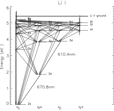
1.8 Grotrian diagram for the 21-level Li atom model. All levels are connected with the Li

ground state by photo-ionization transitions. The astrophysically relevant 670.8 and

610.4 nm lines correspond to the 2s−_{2pand 2p}−_{3dtransitions, respectively. Diagram}

taken from [27].. . . 19

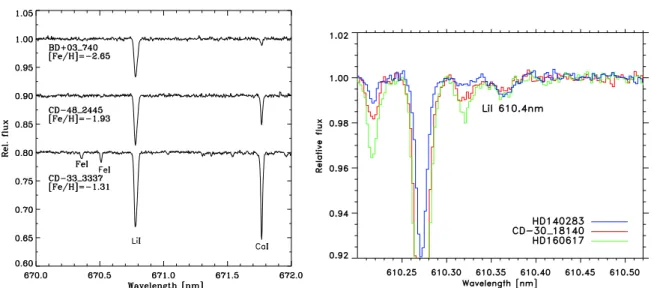
1.9 Left panel: Sample spectra around the Li 670.8 nm line for three metal-poor halo

stars. Plot taken from [20]. Right panel: The region around the Li 610.4 nm for three

metal-poor stars. The Fe610.22 nm, Ca610.27 nm, and Fe610.32 nm lines are also

present in this region. These lines have a different strength in each star. In contrast,

the Li line has a very similar strength in the three stars−_{an illustration of the Spite}

plateau. Plot taken from [28]. . . 21

1.10 Evolution of7_Li,6_{Li, and Be in the Milky Way. The}7_{Li abundance corresponding to}

the baryonic density of the universe derived by WMAP is indicated as dashed

hori-zontal line. The other curves correspond to a simple chemical evolution model where

the metallicity dependent stellar yields component comes from production of 7Li and

6_{Li by GCR. The GCR composition is assumed primary in order to reproduce the Be}

observations. The contribution of the GCR component of6Li is indicated by adashed

curve. Plot taken from [39]. . . 26

2.1 Schematic representation of the combined square nuclear and Coulomb potentials. A projectile incident with energyE< Echas to penetrate the Coulomb barrier in order to

reach the nuclear domain. . . 34

2.2 Dominant energy dependencies for fusion reactions. While both the Maxwell-Boltzmann function and the tunneling probability function, are small in the overlapping region, the

convolution of both functions leads to a peak, the Gamow peak (shadowed area), at

energyE0and width∆E0. . . 36

2.3 Effect of the atomic electron cloud on the Coulomb potential of a bare nucleus (shown in an exaggerated and idealized way). This potential is reduced at all distances and

2.4 Left panel:S(E) factor of D(d,p)T for Hf atT =200◦_{C andT=20}◦_{C, with the deduced}

solubilitiesyandUegiven at each temperature. The curve forT =20◦C represents well

the bareS(E) factor, while the curve forT=200◦_{C includes the electron screening with}

the givenUevalue. Right panel:S(E) factor of D(d,p)T for Pt atT =20◦C and 300◦C,

with the deduced solubilitiesyand Uegiven at each temperature. In both figures, the

curves through the data points are theS(E) fits to these points. Both plots were taken

from [55]. . . 42

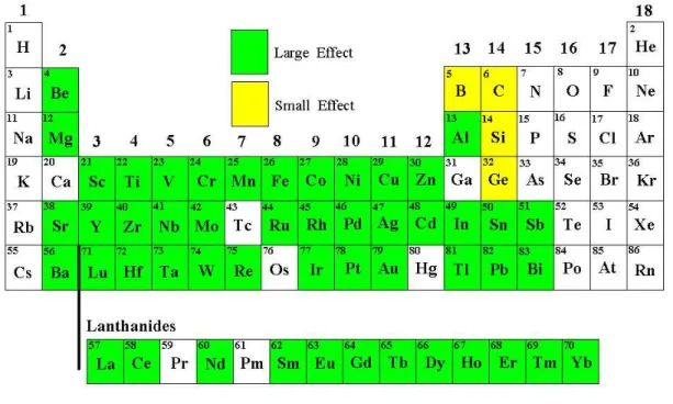
2.5 Periodic table showing the elements studied, where those with lowUe values (Ue<70

eV) are colored yellow and those with highUevalues (Ue >150 eV) are colored green. 43

3.1 S-factor for the7Li(p,α)4He as a function of7Li+p c.m. energy. The experimental points are from Engstleret al. [50] (atomic target: pluses; molecular target: crosses),

Spinkaet al. [59] (solid squares), and Rolfs and Kavanagh [60] (circles). The solid

curve is anR-matrix best fit to the data from Engstleret al. , together with

angular-distribution data also from Engstleret al., andα+αd-wave phase shifts values. The

dashed curve is the best fit when theS-factor data for E≥_{100 keV are from Refs.[59, 60]}

rather than from Ref.[50]. The dotted curves give the corresponding bareS-factor. Plot

taken from [62].. . . 51

3.2 8_{Be level scheme. . . . . 53}

3.3 7_Li(p,α)4_{HeS-factor as a function of}7_{Li+p c.m. energy. The data are taken from Ref.}

[63] (Cassagnou 62), Ref. [64] (Fiedler 67), Ref. [59] (Spinka 71), Ref. [60] (Rolfs

86), Ref. [50] (Engstler 92), and Ref. [61] (Lattuada 01). The solid curve represents

theR-matrix fit done by Descouvemontet al.[58], and the dotted curves represent the

lower and upper 1σlimits. Plot taken from [58]. . . 54

3.4 Left panel: Angular distribution W(E,θ) at representative c.m. energies for the7_Li(p,α)4_He

reaction. Data taken from [50]. Right panel: Energy dependence of the dominant

co-efficient,A2, in the angular distribution for the 7Li(p,α)4He reaction. Data taken from

3.5 S-factor for the 6Li(p,α)3He as a function of6Li+ p c.m. energy. The experimental points are from Engstleret al.[50] (atomic target: pluses; molecular target: crosses);

Marionet al. [66] (solid squares); Shinozukaet al.[69] (triangles); Elwynet al.[68]

(circles). The solid curve is a best fit, based on a cubic form for the bareS-factor, which

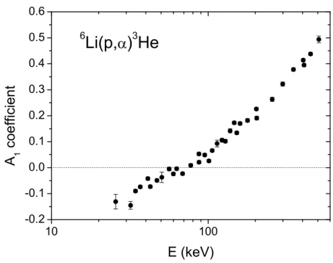
is shown by the dotted curve. Plot taken from [62]. . . 58 3.6 Energy dependence of the dominant coefficient,A1, in the angular distribution for the

6_Li(p,α)3_{He reaction. Data taken from [50]. . . . . 60}

4.1 The excitation function of the27_Al(p,γ)28_{Si reaction atE}

r,lab=992 keV using an Al

tar-get 99.999% pure (Eγ =1.779 MeV). The curve through the data points is to guide the

eye only. Er,lab corresponds to the mid-point on the excitation function curve halfway

between the 12% and 88% height of the net yield. The energy difference between these

points is the energy spread of the beam, 1.1 keV in our case. . . 62 4.2 Schematic diagram of the beam line vacuum system. . . 63 4.3 Top view drawing of target chamber used at ITN. Colour legend: green – steel AISI

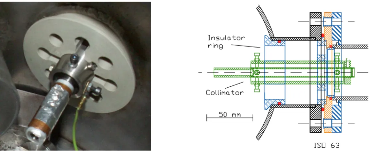
304; orange – other metals; blue – insulator; red – o’rings. . . 64 4.4 Left panel: Photo of collimating system - view from inside the target chamber. Right

panel: drawing of the collimating system and insulating supports. . . 65 4.5 Left panel: Photo of beam stopper - view from inside the target chamber. Right panel:

beam stopper drawing. . . 66 4.6 Number ofα’s detected by each Si detector as a function of its angular position. The

full lines represents the results of the linear fits to the data, as reported in the text. . . . 66 4.7 Left panel: Particle spectrum obtained with the Si detector at an angle of 124◦_by

bom-barding the LiF-Ag target with protons of incident energyEp=1404.5 keV. Right panel:

γ-ray spectrum obtained with the HPGe detector at an angle of 130◦_{by bombarding the}

7_{Li implanted in Al target with protons of incident energyE}

p=894 keV. . . 67

4.8 Left panel: The excitation function of the 11B(p,γ)12C reaction atEr,lab = 163.0 keV

using a thick boron foil. The blue line connecting the data points are an

interpola-tion curve and is to guide the eye only. Right panel: The excitainterpola-tion funcinterpola-tion of the

19_F(p,αγ)16_{O reaction atE}

r,lab=340.5 keV using a thin LiF film. The blue line

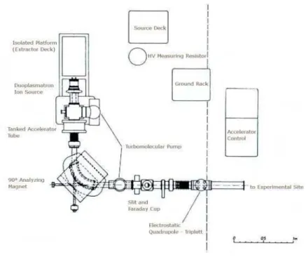
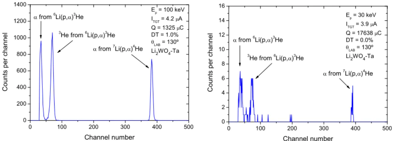
4.9 Schematic diagram of the main components of the 100 kV accelerator at DTL, Bochum. Figure taken from [54]. . . 70 4.10 Schematic view of the target chamber at DTL, Bochum. Figure taken from [54]. . . . 71 4.11 Particle spectra obtained with a Si detector at an angle of 130◦ _{by bombarding the}

Li2WO4 target with protons of incident energyEp=100 keV (left panel) and 30 keV

(right panel). . . 72 4.12 The 1.574 MeV4He+ backscattering spectra of the LiF-Ag target, measured

simulta-neously at two different angles,θlab=94◦and 115◦. . . 73

4.13 The 1.574 MeV4_He+ _{backscattering spectra of the LiF-Ag target, measured at θ}

lab=

115◦_{. Ag plural scattering events (background) subtraction under the} 7_{Li, C, O and F}

peaks. The background events are fitted with exponentials and then subtracted from the

spectrum. . . 74 4.14 The 1.574 MeV4He+ backscattering spectra of the LiF-Ag target, measured at θlab=

115◦_{. Ag plural scattering events (background) subtraction under the} 7_{Li, C, F and O}

peaks. The background events are fitted with anE−α _{dependence under the} 7_{Li peak}

and by two exponentials under the C, O and F peaks. The fitted functions are then

subtracted from the spectrum. . . 75 4.15 The 1.574 MeV4He+_{backscattering spectrum of the LiF-Ag target measured atθ}

lab=115◦

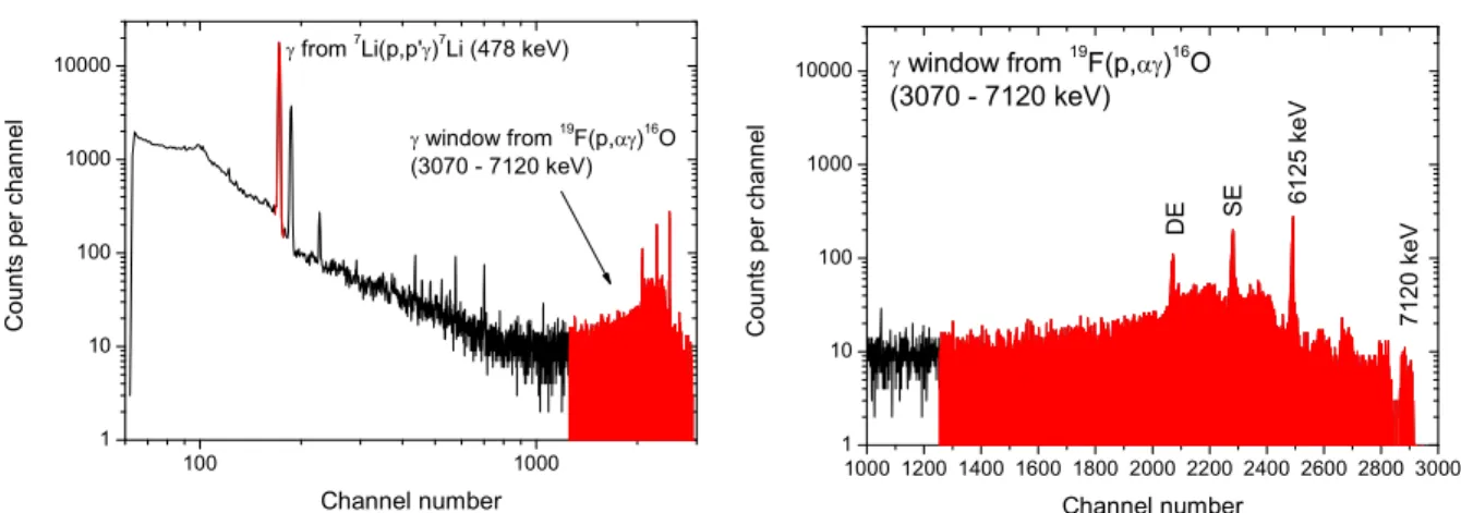
(after background subtraction), and the XRUMP simulated spectrum (red curve). . . . 76 4.16 Left panel: γ-ray spectrum taken from the LiF-Cu target at Elab = 1134 keV. Right

panel: Same spectrum zoomed over the γ window from the 19F(p,αγ)16O reaction.

The SE and DE peaks correspond, respectively, to the single escape and double escape

peaks of the 6125 keV photo peak.. . . 78 4.17 The excitation function of the 19F(p,αγ)16O reaction at Er,lab = 483.6 keV using the

LiF-Cu target. The curve through the data points is to guide the eye only. . . 78 4.18 The Sn-Li alloy phase diagram. Plot taken from [76]. . . 79 4.19 Implantated profile evolution with increasing fluence as predicted by eq. 4.10, for 7Li

implantation into aluminium at 10 keV. The red horizontal line indicates the atomic

4.20 The excitation function of the7Li(p,γ)8Be reaction atEr,lab =441.4 keV using the two

implanted targets and a vacuum evaporated LiF thin target. The quoted uncertainties

are only of statistical nature and the lines through the data points are to guide the eye

only. . . 84 4.21 The 2.0 MeV4He+backscattering spectra of the7Li implanted target, measured atθlab=

140◦_{. The left panel shows theχ}2_{fit to the Al barrier with two exponentials (red curve).}

The right panel shows the RBS spectrum after subtracting the Al barrier with the fitted

exponentials. . . 85 4.22 Left panel: The 2.0 MeV 4He+ backscattering spectrum of the 7Li implanted in Al

target measured atθ_lab=140◦_{(with the Al barrier partially subtracted), and the XRUMP}

simulated spectrum (red curve). Right panel: Original RBS spectrum, superimposed on

the XRUMP fit (red curve). . . 85 4.23 Depth profile of7Li, Al, O and C predicted by the XRUMP fit to the RBS spectrum of

the7Li implanted in Al target. The lines through the data points are to guide the eye only. 86 4.24 Left panel: The excitation function of the 27Al(p,γ)28Si reaction at Er,lab =992 keV

using the Al target before (gray triangles) and after 7Li implantation (blue squares).

Right panel: Comparison of Al depth profiles obtained by the 27Al(p,γ)28Si excitation

function measurement (blue squares) and RBS measurements (orange circles) – see text

for details. . . 88 4.25 The normalized sputtered 7Li+₂ and Al+₂ yield as a function of sputtering time (in

arbi-trary units) for the7Li implanted target obtained with a 4 keV Ar+primary beam in an

O2atmosphere (P=1.0×10−6mbar). The lines through the data points are to guide the

eye only. . . 89 4.26 Left panel: The normalized sputtered H+,7Li+, Na+, Al+and K+yield as a function of

sputtering time (in arbitrary units) for the 7Li implanted target obtained with a 4 keV

Ar+ _{primary beam. Right panel: The normalized sputtered C}−_{, O}−_{, C}+

2 and Cl−yield

as a function of sputtering time (in arbitrary units) for the7Li implanted target obtained

with a 4 keV Ar+_{primary beam. The lines through the data points are to guide the eye}

only. . . 89 4.27 Mg Kα X-rays XPS spectrum that shows the detected photo-emitted electrons as a

4.28 The excitation function of the7Li(α,γ)11B reaction atEr,lab=953 keV using a Pd94.1%Li5.9%

target. The line through the data points is to guide the eye only. . . 91

4.29 7_Li(p,α)4_{He yield [N(}4_{He)/Q] evolution with accumulated charge for the LiF-Cu target,}

at different energies. The white and orange data points correspond to the Si detectors at

124◦ _{and 145}◦_{, respectively. The error bars come from the statistical error on N(}4_He)

counts. . . 94

4.30 7_Li(p,α)4_{He yield [N(}4_{He)/Q] (red circles) and} 6_Li(p,α)3_{He yield [N(}3_{He)/Q] (gray}

squares) evolution with accumulated charge for the Li metal target. The error bars

come from the statistical error on N(3,4He) counts. . . 95 4.31 7_Li(p,α)4_{He yield [N(}4_{He)/Q] (red circles) and} 6_Li(p,α)3_{He yield [N(}3_{He)/Q] (gray}

squares) evolution with accumulated charge for the Pd94.1%Li5.9%target. The error bars

come from the statistical error on N(3,4He) counts. . . 96

5.1 Left panel: Stopping cross section of Li for protons, ǫLi, as a function of Elab in the

energy range 10 – 100 keV. Theǫ_Livalues, given by SRIM [79], wereχ2fitted with a

polynomial function (red line). Right panel: Stopping cross section of Li for protons,

ǫLi, as a function of Elab in the energy range 90 – 1400 keV. TheǫLivalues, given by

SRIM [79], wereχ2fitted with a polynomial function (red line). . . 100

5.2 Schematic scattering event as seen in the laboratory and center-of-mass coordinate sys-tems ilustrating the angles and energies for nonrelativistic inelastic collisions. . . 102

5.3 Angular distributions of the4He particles for the7Li(p,α)4He reaction at the energies indicated. The solid lines represent the result of the Legendre polynomial fits given by

Eqs. 5.24 (blue line ) and 5.25 (red line).. . . 104

5.4 Angular distributions of the4He particles for the7Li(p,α)4He reaction at the energies indicated. The solid lines represent the result of the Legendre polynomial fits given by

Eqs. 5.24 (blue line ) and 5.25 (red line).. . . 105

5.5 Angular distributions of the4He particles for the7Li(p,α)4He reaction at the energies indicated. The solid lines represent the result of the Legendre polynomial fits given by

5.6 Left panel: DeducedA2(E) coefficient as a function of the energy. The solid curve

rep-resents a fourth order polynomial fit to the data. Right panel: DeducedA4(E) coefficient

as a function of the energy. The solid curve represents a linear fit to the data. . . 106 5.7 DeducedA2(E) coefficient as a function of the energy. Comparison with previous works.107

5.8 Energy dependence of the dominant coefficient,A1, in the angular distribution for the 6_Li(p,α)3_{He reaction. Data taken from [50]. The solid curve represents a second order}

polynomial fit to data. . . 108 5.9 Left panel: The S-factor for the 7Li(p,α)4He as a function of 7Li+ p c.m. energy,

measured for the7Li implanted in Al target at 124◦_{(black squares) and 145}◦_(red

cir-cles). Right panel: AveragedS(E) values obtained from the two Si detectors (see text

for details). . . 116 5.10 Left panel: The S-factor for the 7Li(p,α)4He as a function of 7Li+ p c.m. energy,

measured for the LiF-Ag target at 124◦ _{(black squares) and 145}◦ _{(red circles). Right}

panel: AveragedS(E) values obtained from the two Si detectors (see text for details). . 116 5.11 Left panel: The S-factor for the 7Li(p,α)4He as a function of 7Li+ p c.m. energy,

measured for the LiF-Cu target at 124◦ _{(black squares) and 145}◦ _{(red circles). Right}

panel: AveragedS(E) values obtained from the two Si detectors (see text for details). . 117 5.12 Left panel: Astrophysical S(E) factor of7Li(p,α)4He obtained using all targets. Right

panel: Same plot zoomed over the energy interval below 900 keV. . . 117 5.13 Same plot of fig. 5.12, without distinction of target and with a few data points merged

(see text for details). . . 118 5.14 TheS-factor for the7Li(p,α)4He as a function of7Li+p c.m. energy. The experimental

points are from the present work (black squares), from Rolfs and Kavanagh [60] (red

circles), Spinkaet al. [59] (blue triangles), Harmonet al. [84] (green triangles) and

Engstleret al. [50] (pink triangles). . . 119 5.15 Left panel: The S-factor for the 6_Li(p,α)3_{He as a function of} 6_{Li+ p c.m. energy,}

measured for the LiF-Cu target at 124◦ _{(black squares) and 145}◦ _{(red circles). Right}

panel: AveragedS(E) values obtained from the two Si detectors (see text for details).

5.16 TheS-factor for the6Li(p,α)3He as a function of6Li+p c.m. energy. The experimental points are from the present work (black squares) and from Elwynet al. [68] (red circles)

and Engstleret al. [50] (blue triangles). . . 122

5.17 TheS(E)-factor data for the7Li(p,α)4He reaction. The solid curve is a fit with a 3rd-order polynomial function (eq. 5.53). The red portion of the curve defines the fitted

energy region (Ebetween 89.7 and 1740.3 keV – full energy range), and the green

por-tions correspond to the extrapolated curve. P1, P2, P3 and P4 correspond respectively

to parametersa,b,canddof eq. 5.53. . . 124

5.18 TheS(E)-factor data for the7Li(p,α)4He reaction. The solid curve is a fit with a 3rd-order polynomial function (eq. 5.53). The red portion of the curve defines the fitted

energy region (E between 89.7 and 902.2 keV), and the green portions correspond to

the extrapolated curve. P1, P2, P3 and P4 correspond respectively to parametersa,b,c

anddof eq. 5.53. . . 125

5.19 TheS(E)-factor data for the7Li(p,α)4He reaction. The solid curve is a fit with a 3rd-order polynomial function (eq. 5.53). The red portion of the curve defines the fitted

energy region (E between 89.7 and 714.4 keV), and the green portions correspond to

the extrapolated curve. P1, P2, P3 and P4 correspond respectively to parametersa,b,c

anddof eq. 5.53. . . 126

5.20 TheS(E)-factor data for the6Li(p,α)3He reaction. The solid curve is a fit with a 3rd-order polynomial function (eq. 5.53) to data from present work (black squares). P1,

P2, P3 and P4 correspond respectively to parametersa,b,canddof eq. 5.53. . . 128

5.21 TheS(E)-factor data for the6Li(p,α)3He reaction. The solid curve is a fit with a 3rd-order polynomial function (eq. 5.53) to data from present work (black squares) plus

Elwynet al.(1979) [68] data (open circles). P1, P2, P3 and P4 correspond respectively

to parametersa,b,canddof eq. 5.53. . . 129

5.22 TheS(E)-factor data of7_Li(p,α)4_{He for different environments: Li}

2WO4insulator, Li

metal, and Pd94.1%Li5.9% alloy. The solid curves through the data points include the

bareS(E) factor (dotted curve) and the electron screening with theUevalues given in

5.23 TheS(E)-factor data of 6Li(p,α)3He for different environments: Li2WO4insulator, Li

metal, and Pd94.1%Li5.9% alloy. The solid curves through the data points include the

bareS(E) factor (dotted curve) and the electron screening with theUe values given in

the text.. . . 133 5.24 TheS(E)-factor data of7Li(p,α)4He for the two PdLixalloys studied. The solid curves

through the data points include the bare S(E) factor (dotted curve) and the electron

screening with theUe values given in the text. . . 140

6.1 The 1021.8 keV H+ backscattering spectrum of the LiF-Ag target measured atθ_lab =

162◦_{. The red curve shows aχ}2_{fit to the Ag peak with a gaussian plus a gaussian with}

a low energy lorentzian tail, and a two exponential fit to the continuum produced by the

plural scattering events of protons on silver atoms. . . 145 6.2 Zoom of the 1021.8 keV H+backscattering spectrum of the LiF-Ag target measured at

θlab =162◦. The red curve shows aχ2 simultaneous fit to the6Li and7Li peaks. The 6_{Li peak was fitted with a gaussian shape and the} 7_{Li peak was fitted with a gaussian}

plus a gaussian with a low energy lorentzian tail. The lithium fits were done on top of

the continuum and the carbon peak (green curve), fitted with two exponentials and a

gaussian with a low energy lorentzian tail, respectively. See text for details. . . 146 6.3 Cross section of the reaction7Li(p,p)7Li normalised to Rutherford cross section. The

1.1 SBBN results at WMAPΩ_Bh2from different authors. . . 11 1.2 7_{Li observational abundance results from different authors. . . . . 15}

1.3 Influential reactions and their sensitivity to nuclear uncertainties for the production of

4_{He, D,}3_{He and}7_{Li in SBBN. Table taken from [5]. . . . . 29}

1.4 Test of yield sensitivity to reactions rate variations: factor of 10,100,1000 (see text). Table taken from [5]. . . 30

2.1 Energy window (in keV) of the Gamow peak for the6,7Li+p reactions during the BBN (T6between 80 and 800), in the center of the Sun, and in the surface of halo stars. . . . 36

2.2 Electron screening potential energy (in eV) for proton and deuterium induced reactions, in the adiabatic and sudden approximation. Experimental values obtained in laboratory

experiments are also listed with respective references. . . 41

3.1 Legendre polynomials. . . 49 3.2 7_Li(p,α)4_{He: summary table forS}

b(0) andUe. . . 56

3.3 6_Li(p,α)3_{He: summary table forS}

b(0) andUe. . . 59

4.1 Analysing magnet calibration reactions. . . 68 4.2 SRIM simulation results and eq. 4.10 predictions for different metal backings at Elab =

5 and 10 keV.DNmax. gives the fluence necessary to obtain a saturated profile andDI

is the retained fluence (see text for details).. . . 81 4.3 478 keVγ-ray yields produced in the implanted Al, Pb, Sn and Sb with 5×₁₀17 7_Li+_/cm2_. 83

5.1 7_Li(p,α)4_{He reaction: ǫ}

eff(E) 5% variation effects onEandS(E) for the7Li implanted target, andθ_lab =124◦ _{(see details in text). . . . 112}

5.2 6_Li(p,α)3_{He reaction:ǫ}

eff(E) 5% variation effects onEandS(E) for the LiF-Cu target, andθlab =124◦(see details in text). . . 113

5.3 S-factor data for the7Li(p,α)4He reaction. The quoted uncertainties correspond to one standard deviation. . . 120 5.4 S-factor data for the6Li(p,α)3He reaction. The quoted uncertainties correspond to one

standard deviation. . . 121 5.5 Polynomial expansionS(E) = a+b E + c E2 +d E3 fitted to the7_Li(p,α)4_He

reaction S-factor for three different energy regions. The quoted uncertainties correspond to one standard deviation. . . 123 5.6 Polynomial expansionS(E)= a+b E+c E2+d E3fitted to the6_Li(p,α)3_He

re-actionS-factor considering only present work data and considering also Elwyn

et al. (1979) [68] data. The quoted uncertainties correspond to one standard deviation. . . 127 5.7 S-factor data for the7Li(p,α)4He reaction measured for E below 90 keV with the

tar-gets: Li2WO4 insulator, Li metal and Pd94.1%Li5.9%. The quoted uncertainties

corre-spond to one standard deviation. . . 131 5.8 S-factor data for the6Li(p,α)3He reaction measured for E below 90 keV with the

tar-gets: Li2WO4 insulator, Li metal and Pd94.1%Li5.9%. The quoted uncertainties

corre-spond to one standard deviation. . . 131 5.9 7_Li(p,α)4_{He and}6_Li(p,α)3_HeU

e values obtained from theχ2 fits to theS-factor data

for E below 90 keV with the targets: Li2WO4 insulator, Li metal and Pd94.1%Li5.9%.

The quoted uncertainties correspond to one standard deviation. . . 134 5.10 S-factor data for the7_Li(p,α)4_{He reaction measured for E below 90 keV with the}

PdLi0.016%target. The quoted uncertainties correspond to one standard deviation. 141

6.1 Differential cross section of elastic scattering of protons by7Li normalized to rutherford cross section values. The scattering angle is θlab = 162◦. The quoted uncertainties

B.1 Angular distributions,W(E, θ), of the4He particles for the7Li(p,α)4He reaction atE=

1740, 1609 and 1477 keV. The quoted uncertainties are only statistical. . . 166 B.2 Angular distributions,W(E, θ), of the4He particles for the7Li(p,α)4He reaction atE=

1345, 1214 and 1081 keV. The quoted uncertainties are only statistical. . . 167 B.3 Angular distributions,W(E, θ), of the4He particles for the7Li(p,α)4He reaction atE=

949, 817 and 685 keV. The quoted uncertainties are only statistical. . . 168 B.4 Angular distributions,W(E, θ), of the4_{He particles for the}7_Li(p,α)4_{He reaction atE=}

551, 418 and 274 keV. The quoted uncertainties are only statistical. . . 168 B.5 Angular distributions of the4_{He particles for the}7_Li(p,α)4_{He reaction atE=150 and}

80 keV. The quoted uncertainties are only statistical. . . 169 B.6 A2(E) and A4(E) coefficients values obtained fromχ2 fits to the angular distributions

of the4He particles for the7Li(p,α)4He reaction. The quoted uncertainties correspond

to one standard deviation. . . 170

D.1 7_Li(p,α)4_{HeS-factor measured with the}7_{Li implanted in Al target. The quoted}

uncer-tainties correspond to one standard deviation. . . 184 D.2 7_Li(p,α)4_{HeS-factor measured with the LiF-Ag target. The quoted uncertainties}

cor-respond to one standard deviation. . . 185 D.3 7_Li(p,α)4_{HeS-factor measured with the LiF-Cu target. The quoted uncertainties}

cor-respond to one standard deviation. . . 186 D.4 6_Li(p,α)3_{HeS-factor measured with the LiF-Cu target. The quoted uncertainties}

Lithium is one of the most interesting and puzzling elements in the field of nucleosynthesis. Its most abundant isotope,7_{Li, has the rather unique status of requiring three enterely different}

nucleosynthetic processes: Big Bang Nucleosynthesis (BBN), galactic cosmic ray spallation of interstellar matter, and a poorly identified stellar process.

The amount of7_{Li present in stars, among other factors, depends on the rate of the}7_Li(p,α)4_He

reaction. However, very recently, it has been determined that the primordial lithium abundance expected on the basis of7_Li(p,α)4_{He cross section measurements does not match that observed}

in several astrophysical sites such as very old Pop. II stars from the Milky Way halo. For the lighter isotope,6_{Li, there is also no agreement between expected and observed primordial}

abundances.

These discrepancies have triggered a large amount of research in the fields of stellar evolu-tion, cosmology, pre-galactic evolution and nuclear reactions. The accuracy of the predictions given by stellar and primordial nucleosynthesis models depends greatly on the accuracy of the cross sections of reactions that take place in those scenarios, and whose values can be measured in laboratories with particle accelerators. This is the field of experimental nuclear astrophysics, to which this work brings a contribution.

In astrophysical scenarios, charged particles nuclear reactions take place predominantly over the Gamow peak, an energy window situated at very low energies. For these reactions the Coulomb barrier makes these reactions very unlikely at such low energies, often requiring long data collection times with painstaking attention to background.

fully ionized plasma, where electrons move much faster than the nuclei. In a laboratory, an ion beam strikes a neutral atomic (or molecular) target, where electrons are much more confined around the target nucleus. So, due to their different electronic arrangement, electron screening is not the same in a star plasma and in a neutral target. This means that fusion cross sections measured in the laboratory have to be corrected by the electron screening when used as inputs of a stellar or primordial nucleosynthesis model.

Experimental studies of fusion reactions involving light nuclides have shown the expected exponential enhancement of the cross section at low energies. However, the observed enhance-ments were in several cases much larger than could be accounted for from available atomic-physics models. Suggested solutions of the large enhancement including aspects such as stop-ping power or thermal motion were not successful. Recently, an explanation came from a more radical approach, after studying the electron screening in D(d,p)T for deuterated metals, insula-tors, and semiconductors: the large screening, only observed in metals, is due to a star-plasma-like behaviour of the conduction electrons of a metal. This model predicted a temperature de-pendence which was verified with the D(d,p)T study, but also predicted a dede-pendence with the target atomic number and an isotopic independence, which required experimental verification.

This experimental work was the motivation of this thesis. The low energy,Elab ≤ 100 keV, 7_Li(p,α)4_{He and}6_Li(p,α)3_{He reactions cross sections (expressed in terms of the astrophysicalS}

-factor) were measured concurrently in different environments (insulator and metallic targets), and the corresponding electron screenings were determined. A precise quantification of this screening effect requires an equally accurate knowledge of the cross section at higher energies where the electron screening effect is negligible. As the available data was not very accurate and presented discrepancies, a new study of both nuclear reactions at high energy, Elab > 116

keV, was done which included the cross section determination and the measurement of the 7_Li

reaction angular distributions.

The7_Li(p,p)7_{Li differential cross section was also measured in this work. Elastic scattering}

of protons by7_{Li does not directly present an astrophysical interest but is important to describe}

the entrance channel of the 7_Li(p,α)4_{He reaction, and in this view is important for theoretical}

models.

ad-dresses the determination of nuclear reaction rates, including the effects of the Coulomb barrier and electron screening. Chapter 3 presents the status, prior to this work, on the most relevant experimental data for both lithium reactions. The description of the experimental details is given in Chapter 4. It embraces the experimental setups, and details about target preparation and analysis. Chapter 5 describes the analysis used to obtain the astrophysicalS-factor with estimation of associated uncertainties, the results obtained from this analysis and its interpreta-tions. Chapter 6 describes the measurement of the7_Li(p,p)7_{Li reaction, and the results obtained.}

Primordial lithium in the universe

The Big Bang model is a broadly accepted theory for the origin and evolution of the uni-verse. From this model, we know that during the first three minutes of the universe, hydrogen, deuterium, helium-3, helium-4 and trace amounts of lithium were formed. The amount of7_Li

now present in the universe was almost entirely produced here.

This primordial abundance of light elements depends on the density of nucleons (baryons) and on the reaction rate of the weak and the nuclear reactions involved in the production of these elements. From the available measured data, the deduced primordial abundances may be compared with spectroscopic observations.

After the discovery, in 1982, that Pop. II old stars from the Milky Way galactic halo had a near constant lithium abundance, there was a near-universal association of this lithium abun-dance plateau (called Spite plateau) with primordial nucleosynthesis. However, recent and pre-cise measurements of the baryon-to-photon ratio (η) and the detection of the lighter isotope6_Li

in some of the plateau stars, have cast serious doubts over that association. The standard model of the Big Bang with the most recent estimate ofηpredicts a lithium (7_{Li) abundance greater by}

a factor 3 than the value generally attributed to the Spite plateau, and a6_{Li abundance several}

orders of magnitude below the values observed.

1.1

Big Bang Nucleosynthesis

The Big Bang model suggests that 13.7 billion years ago [1], a tremendous explosion, called the Big Bang, initiated the expansion of the universe. Before this explosion, all the matter in the universe was contained in a single point, no more than a few millimeters across. The universe has since expanded from this hot, dense state into the spacious and much cooler environment, which we now inhabit.

When the universe was roughly 1 s old, the temperature had fallen from an initial value greater than 86 MeV (= 1012 _K 1_{) to around 1 MeV, and consisted mostly of photons (γ),}

electron-positron pairs (e−_−e+_{) and particle-antiparticle pairs of all known “flavours” of}

neu-trinos (νe, νµ, ντ). There were also trace amounts of protons (p) and neutrons (n) with a ratio

n/p _≈ 1/6. These baryons reacted with each other forming deuterium through the reaction p+n_→d+γ, but the low binding energy of 2.22 MeV for deuterium combined with the high density of high-energy photons (around 109_{photons per baryon) lead to immediate}

photodisin-tegration of deuterium. Thus, the synthesis of heavier and more stable nuclei such as 4_{He was}

blocked by the fragility of deuterium. Approximately 1 minute after the Big Bang, when the temperature of the universe reached _≈ 0.1 MeV (_≈ 109 _{K), deuterium became stable against}

photodissociation allowing protons and neutrons to undergo a series of nuclear reactions resul-ting predominantly in the production of 4_{He nuclei (99.99 % efficiency) with no free neutrons}

surviving 2_{. Deuterium,} 3_{He and} 7_{Li were also synthetized to a much lower extent, though.}

Since there is no stable element of mass 5, nor of mass 8, additional nucleosynthesis via4_He+

p or4_He+4_{He was not possible. This process of light element production in the early universe}

is known as Standard Big Bang Nucleosynthesis (SBBN) and was first suggested by Alpher and Gamow in 1948 in the so-calledαβγpaper [2]. Based on standard cosmology and particle physics, uniform baryon density, small degree of matter-antimatter asymmetry, and describing gravitation with general relativity, the theory has been strengthened over the last 30+years, on the whole, computing abundances for these light elements comparable to those now observed (or, observable!) in a variety of astrophysical sites (e.g., stars; cool, neutral gas; hot, ionized gas).

1

It is common in astrophysics to use the following temperature-energy relation:E=kBT =8.6171×10−

5

T(eV)

=8.6171×₁₀4T9(eV)=8.6171×10− 2

T9(MeV). 2

The main reactions involved in this process are listed in fig. 1.1.

Figure 1.1: The 12 most important reactions affecting the predictions of the light element abundances (4He, D,3He,7Li).

At the time of4_{He production the universe was an ionized gas (plasma) composed mostly}

of protons, helium nuclei and electrons in thermal equilibrium with the photon sea. As the uni-verse kept expanding, the temperature and density of matter and radiation continued to decrease steadily, dropping in a few minutes well below the levels needed to sustain further nuclear re-actions. When the temperature dropped below 4500 K (379 000 years after the Big Bang [1]), the ions and electrons of the plasma combined, resulting in a neutral gas. With this charge neutralization, the previously opaque universe became transparent3_{, allowing radiation to travel}

unscattered through space, preserving an image of the plasma from which the photons were last scattered. Originally emitted as visible and infrared radiation, this background radiation has been redshifted by a factor of 1500 and is now reaching us primarily in the form of microwaves. These photons, discovered in 1965 by Penzias and Wilson [3], are detected under the form of an almost perfect blackbody spectrum at a temperature of 2.725 K [1] and form the Cosmic Microwave Background, or CMB. It baths the universe almost evenly (see fig. 1.2), showing patterns of tiny temperature differences4_{, which are considered the seeds that generated the}

cosmic structure we see today.

It is worth mentioning, before finishing this section, that even though the Big Bang theory is very successful in explaining the origin of the light elements (SBBN) and the cosmic microwave

3

The main source of opacity was due to free electrons which interacted with photons through Thomson

scatter-ing. 4

Figure 1.2: CMB full-sky map taken by NASA probe WMAP [1]. Colors indicate ’warmer’ (red) and ’cooler’ (blue) spots.

background radiation (CMB), it leaves open a number of important questions. For example, it does not explain why the universe is so non-uniform on smaller scales, i.e., how stars and galaxies came to be. So, a more complete understanding of our universe requires going beyond the Big Bang model. Many cosmologists suspect that Inflation theory, an extension of the Big Bang theory, may provide the framework for explaining some of the puzzles of the Big Bang model [1].

1.1.1

SBBN primordial abundances compared to observations

The primordial yields of light elements are determined by the competition between the ex-pansion rate of the universe (the Hubble constant, H) and the rates of the weak and nuclear reactions. It is the weak interaction, interconverting neutrons and protons, that largely deter-mines the amount of 4_{He which may be synthesized, while the abundances of the other light}

nuclides depend mainly on the nuclear reaction rates which scale with the nucleon (baryon) density. Since the baryon density is always changing as the universe expands, it is convenient to express it in terms of a dimensionless parameter which is either conserved or, changes in a known and calculable fashion. From the very early universe till now the number of baryons in a comoving volume has been preserved and the same is roughly true for photons since the end of BBN5_{. Therefore, the ratio of number densities of baryons (n}

B) and photons (nγ), known as

5

the baryon-to-photon ratio, provides just such a measure of the universal baryon abundance:

η_≡(nB/nγ)0; η10≡ 1010η , (1.1)

where the subscript ‘0’ refers to the present epoch (redshift z=06_).

An equivalent measure of the baryon density is provided by the baryon density parameter,

ΩB, the ratio (at present) of the baryon mass density to the critical density (=9.9×10−30 g/cm3

⇒5.9 protons/m3_{). In terms of the present value of the Hubble parameter, H}

0≡ 100×hkm s−1

Mpc−1_{(=71 km s}−1 _Mpc−1_{), these two measures are related by}

η10 = 274ΩBh2. (1.2)

Fig. 1.3 shows the SBBN predicted abundances of primordial 4_{He (mass fraction) and D,} 3_{He and} 7_{Li (by number relative to H) as a function of baryon-to-photon ratio, η}

10. With the

mapping of the cosmic microwave background and analysis of its temperature anisotropies,η10

has been recently measured with great precision and quite independently of primordial abun-dances by the WMAP NASA probe team, obtaining the valueη10=6.14±0.25 [4] corresponding

toΩ_Bh2 =0.0224_±0.0009 . Combining SBBN results with theη10 value from WMAP (quoted

SBBN+WMAP in the following) we get primordial abundances for D,3_He, 4_{He and} 7_{Li with}

a very small uncertainty, as shown in fig. 1.3, where the WMAP η10 range intersepting the

SBBN yield curves [5] is also represented. Table 1.1 shows the predicted values for the pri-mordial light element abundances at WMAPη10, obtained by different authors. The different

predictions come from different methodologies to fit the experimental data (e.g., normalizations, fitting functions, experimental data used).

The comparison of these predicted abundances with the ones inferred from observational data obtained from a variety of astrophysical sites will allow to confirm the standard model of cosmology or, on the contrary, may open a window for new physics.

electron-positron pairs. This disrupted the equilibrium between photons ande−

−e+_{pairs, since, while positrons} and electrons continued to combine to produce photons, they could no longer be replaced by the reverse reaction.

All positrons were eventually consumed leaving a small excess of electrons (ne/nγ≈10−9) and a constant number

of photons. 6

Redshift, z, is defined as the change in the wavelength,λ, of the light divided by the rest wavelength of the

Figure 1.3:Abundance predictions for standard BBN [5]; the width of the curves give the 1σuncertainty range. The WMAPη₁₀range (η₁₀=6.14±_{0.25) is shown in the vertical (grey) band.}

Starting this comparison with4_{He, we know that its primordial abundance, Y}

P, is relatively

insensitive to the nuclear reaction rates and, therefore, to the baryon density, because of its large binding energy and the gap at mass 5.4_{He observational abundance is probed via emission from}

its optical recombination lines in metal-poor, extragalactic ionized hydrogen (H) regions.

Re-cent observations gave a relatively narrow ranges of abundances: YP=0.2452±0.0015 (Izotov

et al. 1999 [8]), YP = 0.2391±0.0020 (Luridiana et al. 2003 [9]) and, YP = 0.2421±0.0021

(Izotov and Thuan 2003 [10]). Clearly, these results show statistical inconsistencies and are lower than the predicted values of table 1.1. However, this difference of 2₋3% between obser-vation and prediction is relatively modest and it may simply call for further exploration of the systematic effects in the abundance analysis.

Deuterium is considered the ideal baryometer. Deuterium burning, to tritium, 3_{He and}4_He,

Coc et al. 2004 [5] Cyburt 2004 [6] Serpico et al. 2004 [7] D/H (2.60+0.19

−0.17)×10−

5 _(2.55+0.21

−0.20)×10−

5 _(2.58+0.19

−0.16)×10

−5

YP 0.2479±0.0004 0.2485±0.0005 0.2479±0.0004

3_{He/H (1.04±0.04)×10}−5 _{(1.01±0.07)×10}−5 _{(1.03±0.03)×10}−5 7_{Li/H (4.15}+0.49

−0.45)×10−

10 _(4.26+0.91

−0.86×)10−

10 _(4.6+0.4

−0.4)×10

−10

Table 1.1: SBBN results at WMAPΩ_Bh2from different authors.

since deuterium is burned away whenever it is cycled through stars, and no mechanisms are known which may lead to deuterium production, any observed D abundance provides a lower bound to its primordial abundance. For systems at high redshift with very low metallicity, which have experienced a very limited stellar evolution, the observed D abundance should be close to the primordial value. Thus, although there are observations of deuterium in the solar system and the interstellar medium of the Galaxy, which provide lower bounds to the primordial abundance, it is the observations of relic D in a few, high redshift, low metallicity, cosmological clouds along the line of sight of quasars (Lyman-αradiation from the quasars are absorbed and re-emmitted by the deuterium of those clouds) which are most valuable in enabling estimates of its primordial abundance.

The SBBN+WMAP predictions for D/H (listed in table 1.1) are all compatible within errors and are in good agreement with the average value (2.40_±0.3)_×10−5_{of recent D/H observations}

as measured from 6 quasar absorption systems [11] (see fig. 1.4). This agreement strengthens the confidence on the estimated baryonic density of the universe and on the SBBN model itself. However, as shown in fig. 1.4, there is statistically significant scatter of the individual D/H measurements about the average. As deuterium destruction in these clouds is expected to be very low and since the primordial D/H is thought to be isotropic and homogeneous, the scatter is hard to explain. One explanation is that the systematic errors in measuring D/H have been underestimated by the authors. Nevertheless, with only a few quasar absorption systems studied so far, other explanations, such as some early mechanism for deuterium destruction or a non standard BBN, cannot be ruled out. More D/H measurements are needed to understand this scattering problem.

Figure 1.4: Left panel: D/H measurements as a function of log N(H) [N(H) is the column

den-sity in units of cm−2_{] in the absorber where the measurement was made. The hashed region is the}

WMAP+SBBN prediction for D/H from Cocet al.2004 [5]. Right panel: Ratio D/H as a function of

η10. The horizontal stripe represent the average primordial D abundance deduced from observational

data, (2.40±_0.3)×₁₀−5 _{– see text. The vertical stripe represent the (1σuncertainty range)η10limits of}

WMAP.

to that of D, decreasing monotonically withη. Although the SBBN+WMAP predicted values show small uncertainties (see table 1.1), the complex and uncertain evolution of3_{He with stellar}

destruction competing with primordial and stellar production makes difficult the use of current observational data to infer the primordial abundance of3_{He, inhibiting the comparison between}

predicted and observational values [6].

The trend of the BBN-predicted primordial abundance of lithium (almost entirely7_{Li) with} ηis more ‘interesting’ than that of the other light nuclides (see fig. 1.3). The “lithium valley”, centered nearη10 ≈ 2−3, is the result of the competition between production and destruction

in the two paths to mass-7 synthesis. At relatively low baryon abundance (η10 . 2) mass-7 is

mainly synthesized as7_{Li via T(α, γ)}7_{Li. As the baryon abundance increases,} 7_{Li is destroyed}

rapidly by the reaction7_Li(p,α)4_{He. Hence the decrease in}7_{Li/H with increasingηseen (at low} η) in fig. 1.3. Were this the only route to primordial synthesis of mass-7, this monotonic trend would continue, similar to those for D and3_{He. However, mass-7 may also be synthesized via} 3_{He(α, γ)}7_{Be. The}7_{Be will decay to}7_{Li by electron capture (}7_{Be destruction by}7_Be(n,p)7_{Li is}

im-portant because it is mucheasierto destroy7_{Li than}7_{Be. As a result, for relatively high baryon}

abundance (η10 & 3) this latter channel dominates mass-7 production and 7Li/H increases with

increasingη. The WMAP results point towards the highηregion.

From observations of 11 main-sequence stars belonging to the Milky Way Galactic halo 7

Spite & Spite 1982 [12] concluded that the lithium abundance was essentially independent of metallicity for halo stars hotter than 5600 K (the so-called Spite plateau), with the numerical value

7_Li

H =(1.12±0.38)×10

−10_{, (1.3)}

or, equivalently, on the usual astronomical scale8

A(7_{Li)= 2.05}

±0.15 dex. (1.4)

Halo stars, as the ones studied by Spite & Spite, are of Population II, which are the first long-lived stars to have formed after the Big Bang9_{. They are thought to be good lithium ’sources’}

because, contrary to Population I stars, they are not contaminated with elements produced in earlier generation of stars (i.e., have low metal abundance). However, the elderness of these stars can also pose some problems, as some poorly known stellar mechanism(s) may have altered their lithium abundances by an uncertain amount which is not noticeable in our time scale. We will be back to this subject later in this chapter.

Now, more than two decades of measurements has followed since Spite & Spite first results, increasing the number of stars observed and the range of metallicity that they span, confirming a plateau in the warmer (T & 5600 K) and more metal-poor ([Fe/H] . ₋ 1.3) 10 halo stars.

Maurice, Spite, and Spite 1984 [13] showed that the dominant isotope in the plateau was 7_Li:

a limit6_Li/7_{Li< 0.1 was set for a couple of stars. Ryan, Norris, and Beers 1999 [14] showed}

that the Spite plateau is very “thin”, with an intrinsic star-to-star scatter in derived lithium

7

The galactic halo is a spheroidal region of space surrounding spiral galaxies, like the Milky Way. 8

A(X)≡_{log (}nX/nH)+12, wherenXandnHstand for the number density of atoms of elementXand atoms of

hydrogen, respectively; the term “dex” stands for decimal exponent. 9

In fact, there are speculations about a new kind of stars, very massive and short lived, called Population III

stars which are believed to have been formed in the early universe, before Population II stars. They have not been

observed directly, but are thought to be the components of faint blue galaxies. The low-metallicity Population II

stars are thought to contain the metals produced by population III stars. 10

[A/B]=log(nA/nB)−log(nA/nB)⊙, wherenAandnBstands for the number density of atoms of element A and