A Work Project, presented as part of the requirements for the Award of a Master Degree in Finance from the NOVA School of Business And Economics
ESTIMATION OF CREDIT RISK FOR MORTGAGE PORTFOLIOS: EVALUATING FEATURE IMPORTANCE FOR CREDIT RISK MODELING
Field Lab Project Nova SBE & Moody’s Analytics
Jo˜ao Pedro Cavaleiro Dos SANTOS, 23915
A project carried out on the Master in Finance Program, under the supervision of:
Moody’s Analytics Advisors
Dr Bahar KARTALCIKLAR, PhD, Risk Modeller - Content Solutions Dr Petr ZEMCIK, Senior Director - Content Solutions
Carlos CASTRO, Senior Director - Economics and Structured Analytics
Faculty Advisor Professor Jo˜ao Pedro PEREIRA
Feature Selection
Prior to model development, certain variables had to be removed in order to reduce the number of potential drivers and eliminating noise from irrelevant variables. Models with a lower number of variables can be easier to understand and to apply, while having 8-15 variables grant the model stability, whose predictive power will be consistent even if one or two variables are to change, as suggested by Siddiqi (2006).
At this stage, the data set for the Italian mortgage market had over 71 features, where 36 were categorical and 35 continuous features, all available in Table A.7.
The process of feature selection was done in different steps: first performing an univariate analysis for each feature, then clustering similar variables in order to remove highly correlated potential drivers. Afterwards, we created bins for every variable, helping us remove features that have multiple insignificant bins.
Univariate Analysis
Univariate analysis is conducted with the purpose of understanding the effect of a single factor to the final target variable, in our case, the default chance of a certain loan. Although the results that we obtained do not represent the full effect of any individual feature and the target variable, as it ignores relationships between different features, this analysis is used as a starting point for our selection to remove factors that are very obviously not relevant with our target variable.
For continuous features, we will use the Gini coefficient, which is a measure of statistical dispersion. When this coefficient is used in the context of a logistic regression, it measures the ability of a model to distinguish between good and bad instances (defaults and performing loans), compared to random selection. Hence, a higher Gini index indicates a better predictive model, while a coefficient of 0 indicates that the model is as good as a random selection model, being also possible that the model has a negative Gini coefficient, thus decreasing predictive power for the model.
Categorical features will be removed according to their Information Value (IV). IV is a mea-sure of predictive power that a model has given a binary target variable. The IV of a predictor
variable measures the amount of information that said feature has for separating good and bad. The higher the IV is, the better predictor the variable is. Nevertheless, this measure also does not consider the relationship that some different features might have, which will not be a prob-lem as we are performing only an univariate analysis. Furthermore, it is important to note that high IV scores might be influenced by high number of categories, as the total IV score of a feature is the sum of the IV of every category, so further analyses will be performed in order to maintain the most valuable features for our final models.
IV =
n
∑
i
(DistributionGoodi− DistributionBadi) × ln(DistributionGoodi
DistributionBadi ) (1)
Where the distribution of good(bad) is the number of good(bad) instances observed in the category i out of the n categories that a certain feature has, divided by the total number of good(bad) cases.
In order to obtain the IV and Gini coefficients for categorical and numerical variables, re-spectively, a logistic regression only composed by the target variable and each feature (individ-ually) is computed. Continuous variables with a Gini coefficient lower than 0% are eliminated, while for categorical variables, the threshold of 0.01 was set as the bare minimum of Informa-tion Value for a feature to be kept in our model for the next stage, as it is the minimum value for the variable to be considered to add any kind of predictive power.
From the constraints set in this subsection for the minimum values for Gini and IV coeffi-cients that a feature had to had to not be removed, 1 continuous and 14 categorical variables were dropped. Please find the list of eliminated features in Table A.8 in the Appendix.
Reduction of Continuous Variables through Clustering
For the remainder continuous variables, a cluster analysis was conducted, allowing for an even further reduction of the number of features present in the dataset. Clustering is known as an unsupervised classification method, which, in this case, is used to assess collinearity and redundancy, grouping highly similar/correlated variables into clusters, which then can be used to removed redundant features. Hence, one variable per cluster will be selected to be kept, while the others will be removed, prioritising features with higher Gini coefficient. Economic
intuition is also an important factor to consider when deciding which set of variables should be kept for the next phase of feature selection. For some clusters, more than one variable was selected due to business input or economic intuition.
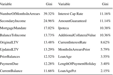
The chosen clustering algorithm grouped the variables based on the Squared Spearman Cor-relation coefficients, as per Moody’s Recommendation, is used to measure the degree of asso-ciation between two variables, detecting monotonic and nonlinear relationships. With this in mind, we split all of the remaining variables into 15 clusters, which allowed us to reduce the number of continuous variables down to 17. The list of variables that were kept in this phase can be found in Table 4.
Table 4: List of continuous variables after the clustering analysis.
Variable Gini Variable Gini
NumberOfMonthsInArrears 39.32% Interest Cap Rate 11.16% SecondaryIncome 24.96% AmountGuaranteed 11.14% MortgageMandate 17.02% Ipoteca 10.38% BalanceToIncome 13.73% AdditionalCollateralValue 10.36% OriginalLTV 13.48% CurrentInterestRate 8.62% UpdatedLTV 13.29% MonthsInArrearsPrior 5.79% PriorBalances 12.52% LoanAge 3.55% PaymentDue 12.28% LengthOfPaymentHoliday 3.40% CurrentBalance 11.66% LoanAgePct 2.15%
It is important to note that NumberofMonthsInArrears will be transformed into a categorical variable, as it only has 3 possible outcomes, current loan, 30 days past due or 60 days past due. However, it is relevant to keep it in at this stage of clustering for continuous variables, as it was used to reduce highly correlated variables.
Correlation Analysis for Categorical Variables
In this section, in order to reduce the number of categorical drivers, variables that are highly correlated with others are removed. For this process, it will be used the Cramer’s V measure of association between two nominal variables. The Cramer’s V value for two variables can range from 0 to 1, where values of 0.5 and above are considered to indicate high correlation between
these two variables.
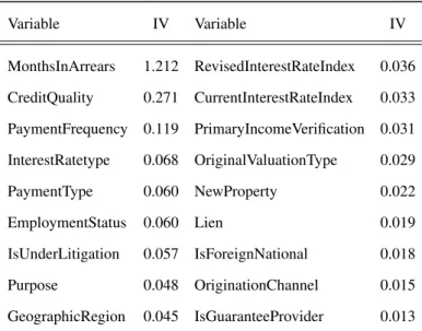
After computing the Cramer’s V for every pair of the remaining 20 categorical variables, the pairs for which this measure was above 0.5 were isolated. Out of this list, economic intuition, business input and each variable’s Information Value is used as a factor to decide which features to keep and which ones to remove. There were only 4 highly correlated pairs of variables, which resulted in the removal of 2 features. The list of categorical features after this analysis can be found in Table 5.
Table 5: List of categorical variables after the correlation analysis.
Variable IV Variable IV MonthsInArrears 1.212 RevisedInterestRateIndex 0.036 CreditQuality 0.271 CurrentInterestRateIndex 0.033 PaymentFrequency 0.119 PrimaryIncomeVerification 0.031 InterestRatetype 0.068 OriginalValuationType 0.029 PaymentType 0.060 NewProperty 0.022 EmploymentStatus 0.060 Lien 0.019 IsUnderLitigation 0.057 IsForeignNational 0.018 Purpose 0.048 OriginationChannel 0.015 GeographicRegion 0.045 IsGuaranteeProvider 0.013
Two other variables were removed at this stage, not because of correlation but due to the economic intuition and from expert input. First we removed Loan Status as, given the dynamic nature of this variable, the status at the cut off date might not be representative of the actual status of the loan in that moment. Originator was also removed as, due to economic intuition, this should not contain any predictive power
Variable Binning
The logistic regression assumes a linear relationship between the target variable and ex-planatory feature, which can be incorrect in some cases, decreasing its potential performance. As such, binning the values of the potential driver features will enable the model to give differ-ent coefficidiffer-ents to each bin, thus allowing it to make the most out of each variable: for those with a linear relationship with the target variable, the model will give incremental coefficients to the
bins of a variable, while for non-linear relationships, the model can measure the appropriate co-efficient for each bin. Hence, all the potential continuous drivers are converted into categorical variables through binning, in accordance to the economic value of each bin and their respective default rate trend. We will also be conducting this process to categorical variables.
For continuous variables, the process usually is based on multiple iterations in order to find the ideal breaks for each bin, while trying to create distinguishable bins in terms of default rate trend, requiring a mix of expert judgement and statistical measures. Some conditions have to be met in order to guarantee that the final bins are statistically well defined:
1. Each bin contains sufficient number of observations so that the estimates are robust. 2. Default rates among the different bins of a variable are in concordance with the economic
intuition of the relationship of the feature and the target variable.
3. Optimum discriminatory power is achieved, given any peculiar aspect/trend of the driver. 4. The coefficients estimates of the multivariate regression should match the default rate
trend among the bins of any variable.
However, with the help of Moody’s Analytics, we were able to run this process using their proprietary binning algorithm. The algorithm uses Information Value as the measure of dis-criminatory power of each category, splitting each driver into a maximum of 10 bins, taking also into consideration the sample size of each group. After obtaining the initial results from Moody’s algorithm, further groups were made in order to improve our initial results, respecting default rate trends per bin and economic intuition behind the binned feature and the dependent variable.
Although categorical variables are already in the format needed to create a scorecard, they will also be subject to further binning. For the binning to be performed, we combined bins that had similar default rate trends, while having the economic intuition behind the variable in consideration, as we do not want to group opposite categories in economic sense just because they have similar default rate trends.
Binning Categorical Variables
To reach the final bins for the categorical variables, different categories with similar default rate trends were grouped, a process iterated for multiple times in order to find the most adequate bins for each variable, while maintaining differentiated default rate trends among different bins. In the process of creating new bins for the categorical variables, 6 variables are removed, some by expert recommendation, while others by having insignificant differences in the default rate trend between different bins or low IV coefficients. Such variables are: CurrentIntere-stRateIndex, OriginalValuationType, RevisedIntereCurrentIntere-stRateIndex, PrimaryIncomeVerification, Lien and IsForeignNational.
Please refer to Table A.9 in the appendix for the final binned categorical variables and the associated bins.
Moody’s Auto Binning Algorithm
Moody’s auto binning algorithm was provided to the group in order to facilitate the process of binning for continuous variables. The algorithm treats this procedure as an optimisation problem, which can be described as:
max
bins {Per f ormanceMeasure(IVorGiniCoe f f icient)} (2)
The optimisation problem is subject to:
1. The relationship with the dependent variable, either monotonic or quadratic, needs to be reflected among different bins
2. Confidence intervals of the default rate for each bin are not overlapping. 3. Final solution is robust on the testing dataset.
The approach followed by the auto binning algorithm from Moody’s is split in 5 different parts:
1. Define the grid of potential boundaries for the bins.
2. Split the variable into two bins, using the boundary that maximises the selected perfor-mance measure.
3. Split again and continue doing so until n bins, at each step selecting the intervals that maximize the performance measure.
4. In every new split, test and combine potential bins if the confidence interval for the default rate is overlapping.
5. The algorithm will stop splitting only when one of the two following conditions are met: (a) If the variable reaches the pre-specified maximum number of possible splits. (b) If there are no other candidate boundaries which could achieve a better performance
measure.
IV score was the performance measure selected for the algorithm, setting the maximum number of bins to be created as 10. After some inspection and analysis of the results from Moody’s algorithm, some bins were combined due to having close default rate trends. In the process, two variables were removed, Payment Due and Secondary Income. Payment Due’s default rate trend did not follow economic intuition regarding the relationship of this feature and the target variable, while Secondary Income had 90% of missing values in the dataset, making it hard to take conclusions from the small subset of data per remaining bin. Secondary Income is also being reflected, when available, in Balance-To-Income, which also makes more economic sense than just the absolute value of income, as the relative weight of the mortgage in an individual’s income is more revealing than just the total value of income or current balance. The final bins for the remaining continuous features can be found in Table A.10 on the Appendix.
Model Driven Feature Selection
In this section, we run two statistical models, where the results from these tests will be used as guidelines for feature selection and further removal of variables due to their low importance for the model. Additionally, the optimal order of feature entrance for the final models can be analysed, as the order used by the model will impact the coefficient for every variable, and as a consequence, the performance metrics of each model.
This procedure consists of three steps, after which it is possible to obtain the final list of variables for the logistic regression and the machine learning model.
1. Run a LASSO Regression with every potential feature and identify the first ten variables that are selected to enter the model.
2. Use a forward stepwise regression and rank all of the potential drivers in terms of their contribution to the overall Gini of the model.
3. Eliminate drivers based on multiple criteria, such as coefficient p-values, coefficient sta-bility throughout training and test datasets, consistency between feature coefficients and the default rate trends, and finally, economic intuition.
The LASSO method, also known as Least Absolute Shrinkage and Selection Operator, is a regression analysis that can be used for feature selection and regularization, considering the importance of each variable to explain the target feature. This technique was introduced by Tibshirani (2019) and has been widely used in different fields of study, being also popular among Machine Learning practitioners. LASSO introduces a penalty factor to every feature, which will be able to shrink the coefficient of some variables to 0, while for others, LASSO will only decrease its β . This is done by maximizing a variant of a log-likelihood function, shown in Equation 3, which uses the penalty factor and penalizes candidate models with more parameters. The penalty factor, λ , is a hyper parameter that can be controlled by the user before running the LASSO regression. A λ of 0 means no penalty factor, thus every feature is considered by the model, while a high λ will eliminate most of the variables, sometimes all of them.
LASSOln (L) =
∑
i
[Badi× ln (Λ(x0iβ )) + (1 − Badi) × ln (1 − Λ(x0iβ ))] + λ ×
∑
j|βj| (3)
In order to get the first ten variables, the LASSO regression was ran multiple times, where the first iteration had a very high λ value, thus eliminating most of the variables, while each subsequent computation had a lower penalty factor value, until our model was composed by 10 variables. Most of the features selected through the LASSO method were already being considered after our initial feature selection process, thus none of these drivers will be added to the list of variables that will be used to run the stepwise algorithm. The results can be seen in Table A.11, on the Appendix.
The second step of the feature selection procedure using statistical models is the forward stepwise regression. This type of regression starts with an empty model, based on a simple logistic regression, and adds new variables, one by one. At each forward step, i.e. each iteration in which a new variable is added, the feature selected to be part of the model is the one that increases the performance of the model the most. The performance metric used to optimize the stepwise regression can be selected by the user. In this case, the Gini coefficient is the target performance measure. Results are shown in Table A.12.
As suggested by previous literature on the topic, such as the works of Thompson (1995) and McNeish (2015), although stepwise regression models originate an ordered list of features that best fits the training data, it does not necessarily reflect the best overall entrance order for every dataset. As a result, instead of making decisions strictly based on the statistical results, we will use a combination of these, with other important aspects of the data, to proceed with feature elimination. The adopted criteria will be:
1. Economic Theory: The relationship between the explanatory variable and the target vari-able should have an economic sense.
2. Statistical robustness: The coefficient of the variable should be statistically significant at a 1% level, while also reflecting the true direction and magnitude of the relationship suggested by economic theory.
3. Practicality: An explanatory variable should be defined in a clear way and it must be accessible by most institutions.
4. Mix of different information: The model should account for different loan, borrower and collateral characteristics.
As mentioned in Section , 8 to 15 is the optimal number of features for a model. Taking Moody’s expertise as well as Siddiqi (2006) into account, we set 10 as the target number of variables for our final models. Thus, 17 variables are further eliminated, which can be seen in Table A.13, where the explanation behind the elimination of each one is presented.
Final List of Variables
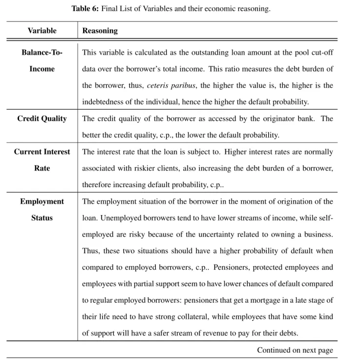
The final list of variables counts 10 different features, covering information from the bor-rower and the loan, using dynamic fields, accessing changes in property value, thus, considering changes in the collateral, but also fields with information from the moment of origination. These features and the economic reasoning behind each is presented in Table 6.
Table 6: Final List of Variables and their economic reasoning.
Variable Reasoning
Balance-To-Income
This variable is calculated as the outstanding loan amount at the pool cut-off
data over the borrower’s total income. This ratio measures the debt burden of the borrower, thus, ceteris paribus, the higher the value is, the higher is the
indebtedness of the individual, hence the higher the default probability.
Credit Quality The credit quality of the borrower as accessed by the originator bank. The
better the credit quality, c.p., the lower the default probability.
Current Interest
Rate
The interest rate that the loan is subject to. Higher interest rates are normally
associated with riskier clients, also increasing the debt burden of a borrower, therefore increasing default probability, c.p..
Employment
Status
The employment situation of the borrower in the moment of origination of the loan. Unemployed borrowers tend to have lower streams of income, while
self-employed are risky because of the uncertainty related to owning a business.
Thus, these two situations should have a higher probability of default when compared to employed borrowers, c.p.. Pensioners, protected employees and
employees with partial support seem to have lower chances of default compared to regular employed borrowers: pensioners that get a mortgage in a late stage of
their life need to have strong collateral, while employees that have some kind
of support will have a safer stream of revenue to pay for their debts.
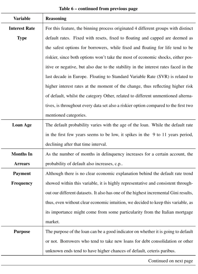
Table 6 – continued from previous page
Variable Reasoning
Interest Rate
Type
For this feature, the binning process originated 4 different groups with distinct
default rates. Fixed with resets, fixed to floating and capped are deemed as the safest options for borrowers, while fixed and floating for life tend to be
riskier, since both options won’t take the most of economic shocks, either
pos-itive or negative, but also due to the stability in the interest rates faced in the last decade in Europe. Floating to Standard Variable Rate (SVR) is related to
higher interest rates at the moment of the change, thus reflecting higher risk
of default, whilst the category Other, related to different unmentioned alterna-tives, is throughout every data set also a riskier option compared to the first two
mentioned categories.
Loan Age The default probability varies with the age of the loan. While the default rate
in the first few years seems to be low, it spikes in the 9 to 11 years period, declining after that time interval.
Months In
Arrears
As the number of months in delinquency increases for a certain account, the probability of default also increases, c.p..
Payment
Frequency
Although there is no clear economic explanation behind the default rate trend showed within this variable, it is highly representative and consistent
through-out our different datasets. It also has one of the highest incremental Gini results, thus, even without clear economic intuition, we decided to keep this variable, as
its importance might come from some particularity from the Italian mortgage
market.
Purpose The purpose of the loan can be a good indicator on whether it is going to default
or not. Borrowers who tend to take new loans for debt consolidation or other unknown ends tend to have higher chances of default, ceteris paribus.
Table 6 – continued from previous page
Variable Reasoning
Updated
Loan-To-Value
The updated LTV is a ratio that measures the total equity that a borrower has
in their home. This variable takes into consideration both the decrease in the outstanding balance of the loan and the macroeconomic environment for that
specific area. Borrowers with higher equity in their homes have lower
probabil-ities to default, hence, c.p., an increase in the updated LTV value should equate an increase in the probability of default.
Categorical Variables
A categorical variable contains, as the name already indicates, several categories. In the raw dataset, these categories are usually shown as strings. Like any mathematical model, neither the logistic regression nor most of the machine learning models can handle string values. Therefore, the strings have to be converted to a numerical representation. Since the categories do not necessarily follow an internal order, it is not possible to just replace the categories with numbers.
One-Hot-Encoding
The classical approach to encode categorical variables is to use the dummy or one-hot en-coding approach. With this approach, every category is converted into a new feature. The feature value becomes one if the category exists and zero otherwise. Be aware that a variable with n categories will lead to n-1 new features since one category is always dropped to avoid multicollinearity problems. This can make, depending on the model, the interpretation of the results more difficult. In addition, this approach generates a big, sparse matrix which is in computational terms difficult to handle.
Weight-of-Evidence
The Weight-of-Evidence encoding is part of target based encoders. Every category is con-verted into a number, which is based on the target variable.
WoE = ln(DistributionGoodi
DistributionBadi ) (4)
This formula follows the same definition as the IV in Section . The WoE is zero in case the category does not contain any information value. If the distribution of bads > goods, the WoE is negative, otherwise it is positive. Therefore, the WoE encoding introduces a meaningful order into the features which the model can learn. This encoding does not suffer from the sparsity problem. In our case, it is especially used for the machine learning model to speed up the computation of the model. Also, with this encoding, it is possible to visualize the importance of every category relative to the remaining ones.
Multicollinearity of the final features
Multicollinearity is a issue in statistics that can occur in a multiple regression model. This problem is defined by the fact that one of the predictor variables can be linearly predicted from the other features with a substantial degree of accuracy. Although this does not affect the predictability power of the model, it can affect the coefficients of single estimators, thus affecting the ability to take conclusions from the way the final models evaluate certain features used.
To address this problem, we performed the variance inflation factor (VIF) analysis. Since the final set of variables is constituted only by binned features, thus interpreted by the model as categorical variables, generalised VIF (GVIF) is the right measure to use for those features with more than 2 categories, instead of a linear VIF, as evidenced by previous literature on the topic by Fox and Monette (1992). To then compare the results from the GVIF to the linear VIF for features with only two categories, one can raise the GVIF value to the power of 1/(2 ∗ d f ), where the d f is the number of degrees of freedom, in this case, the number of categories. The critical number accepted as an indicator of multicollinearity is a VIF value above 4.0, as suggested by Hair (2014), thus, it is possible to conclude that none of the variables present in the final considered list of drives, suffer from multicollinearity, as presented in the Table 7.
Table 7: Multicollinearity test for the final 10 variables.
Variable GVIF df GV IF[1/(2 × d f )] Months In Arrears 1.284 2 1.065 Payment Frequency 1.843 3 1.107 Credit Quality 1.170 4 1.020
Updated LTV 1.677 5 1.053
Current Interest Rate 1.140 4 1.017 Interest Rate Type 1.398 3 1.057 Employment Status 1.172 2 1.041
Purpose 1.104 2 1.025
Loan Age 1.731 3 1.096